Investigation of the Environmentally-Friendly Refrigerant R152a for Air Conditioning Purposes

Abstract

Heat pumps are efficient and well-established technologies for providing the proper cooling load in the building sector. The objective of this work is the parametric investigation of a heat pump operating with the promising refrigerant R152a for different operating conditions. More specifically, the heat pump is studied for different ambient temperatures, different indoor temperatures and various compressor rotational speeds. The cooling capacity and the coefficient of performance (COP) are the most important parameters which calculated in every scenario. A detailed model is developed in Engineering Equations Solver (EES) and it is validated with literature data. According to the final results, the system can operate in nominal conditions with 5 kW cooling capacity and a COP equal to 6.46. It is found that the COP can be ranged from 4 to 12 and the cooling capacity, while the cooling capacity can reach up to 9 kW. Moreover, a regression equation about the performance of the system is suggested. The obtained results indicate that the use of the R152a leads to high performance and so it can be an environmentally friendly choice for the cooling systems.

1. Introduction

Refrigeration is responsible for the 20% of the global energy consumption [1]. Moreover, the refrigeration process is associated with a series of environmental problems such as the ozone layer depletion and the global warming phenomenon due to the harmful refrigerants [2]. Therefore, there is a need for establishing a refrigeration system with high efficiency and with environmentally-friendly refrigerants [3,4]. According to the European Parliament Directive 517/2014 [5], the use of refrigerants with high global warming potential (GWP) has to be reduced. A general limit in the GWP can be selected at 150 [5], especially for the domestic refrigeration systems and so the use of refrigerants with lower GWP has to be used in the new systems or to replace the existing refrigerants.

At this time, the most usual refrigerants are the R134a and the R404a [6] which have GWP equal to 1430 and 3922 respectively. The next generation of the refrigerants have to be friendlier to the environment and so a lot of interest has been focused on R32 with GWP = 675. However, this refrigerant has a medium and not a low GWP; a fact that creates a great criticism about this [1]. The alternative refrigerant R152a presents GWP = 138 and it is a promising choice according to this criterion. However, it presents relatively higher flammability and it belongs to the A2 ASHRAE group. The refrigerants R1234yf and R1234ze have GWP equal to 4 and 6 respectively and they are good choices, yet their chemical stability problems for long-term operation and their high costs make their utilization questionable. The last and the most promising category for the future are the natural refrigerants which have extremely low GWP. The R717 (NH₃) is a promising refrigerant but it is toxic (B1 ASHRAE group). The R290 (propane) and the R600a (iso-butane) are also natural refrigerants but they have high flammability (A3 ASHRAE group). The last choice is CO₂ which has GWP = 1 and it is not flammable and toxic, but it has a low critical temperature (~31 °C) which leads to transcritical cycle with relatively low efficiency and high-pressure levels.

Table 1. Refrigerants and their characteristics [7,8,9]. GWP: global warming potential; COP: coefficient of performance.

Working Fluids	Classification	GWP	ASHRAE GROUP	Cost ($/kg)	Limitations
R134a	HFC	1120	A1	5.3	High GWP
R404a	HFC	3922	A1	3.5	High GWP
R152a	HFC	138	A2	1.5	Medium flammability, Low GWP
R32	HFC	677	A2L	3.0	Low flammability, Medium GWP
R1234yf	HFO	<1	A2L	88	Low flammability, Stability issues
R1234ze	HFO	<1	A2L	90	Low flammability, Stability issues
R717 (NH3)	Natural refrigerant	<1	B1	1.5	Toxicity
R744 (CO2)	Natural refrigerant	1	A1	0.7	Low COP
R290 (Propane)	HC (Natural refrigerant)	3	A3	1.3	High flammability
R600a (Iso-butane)	HC (Natural refrigerant)	4	A3	2.0	High flammability

summarizes the previous refrigerants and their characteristics [7,8,9].

The previous analysis indicates that there is no optimum refrigerant without any drawback. The use of CO₂ seems to be a promising choice for the future, especially with the modified system with parallel compression, subcooling, and ejector devices [10,11] but there is a need for efficiency enhancement and creating certified personnel [1]. Among the HFC, the use of R152a seems to be a promising choice because of the low GWP which is lower than 150. Only the flammability problems have to be faced in order to establish it. However, it is important to state that R152a belongs to the A2 category and it is less flammable than the R290 and R600a which are also promising and used refrigerants. Therefore, the use of R152a has to be performed with experienced personnel and with the proper safety rules.

The last years, a lot of studies have been conducted about the use of the R152a and they compare it with the existing refrigerants and with other promising. Also, it is useful to state that the R152a is a component in many blends (for instance R444A). Bolaji [12] studied a simple refrigeration system with R152a, R134a and R32. It is found that the use of R152a leads to 8.5% higher coefficient of performance (COP) than R134a, while R32 is the less efficient refrigerant. Moreover, Nie et al. [13] found the R152a more efficient than R134a, R143a, and R32. Cabello et al. [14] examined the use of R152a as a substitute for R134a for the system with and without an internal heat exchanger. They found 13% higher COP with R152a, while a decrease in the cooling capacity. Sanchez et al. [15] examined various refrigerants and they found that R152a is more efficient than R134a, R600a, R1234yf, and R1234ze. However, they found the R290 to be the most efficient working fluid but they highlighted its high flammability and the need for a stronger electrical motor, two factors which make it unsuitable for a direct drop-in alternative of R134a. They finally concluded that the R152a and the R1234yf are the most promising choices for substituting the R134a. Moreover, it can be said that Perez-Garcia et al. [16] stated that the use of the R152a can be performed with the use of a secondary loop for safety reasons and for facing the flammability issues. The use of R152a in cascade configurations with CO₂ in the low stage is a promising choice which has also been examined. Cabello et al. [17] proved that the substitution of R134a refrigerant with R152a is possible in a cascade cycle with CO₂. They performed experimental work and they found similar performance with both configurations and also they stated that the system had worked about two months without problems after the use of R152a. In another work, Yang et al. [18] found that the use of R152a in a cascade system with CO₂ is more efficient than the use of R134a/CO₂ and R124/CO₂ cascade systems.

The previous literature review indicates that the R152a is one of the most promising refrigerants for the future refrigeration machines. The existing studies show high performance and good compatibility with the existing installations. Therefore, there is a need for deeper investigation of this working fluid. In this direction, this study is a detailed analysis of a cooling system with R152a in order to determine its performance and its cooling capacity in different operating conditions. The novelty of this investigation is based on the different examined operating scenarios and on the development of a regression model for the prediction of the system performance. Moreover, it has to be said that there is a lack of studies about the investigation of R152a in the cooling system for the building sector. This work is conducted with a developed model in Engineering Equation Solver (EES) [19] which is validated using literature data [20].

2. Material and Methods

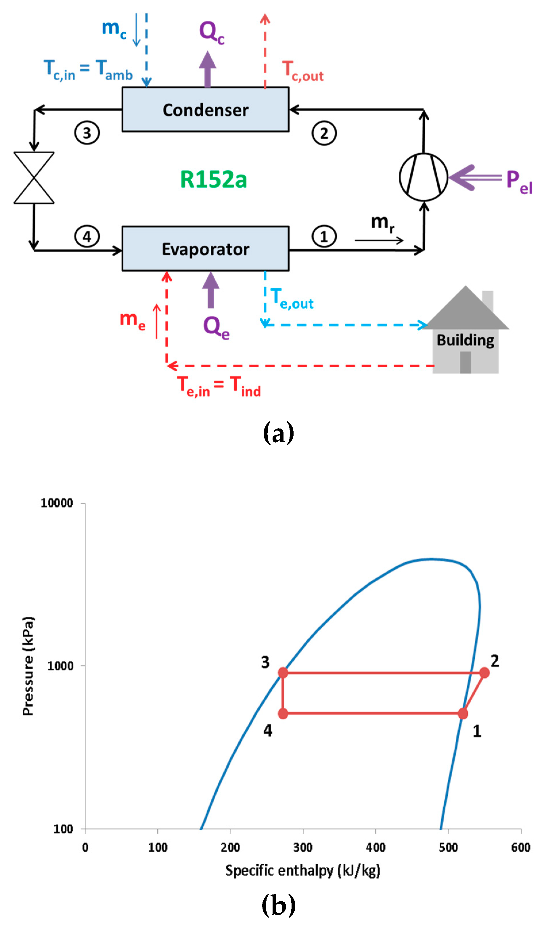
2.1. Examined System

In this work, a simple heat pump system for the cooling of a building is investigated, as Figure 1a illustrates. R152a is the examined working fluid which is a relatively environmentally-friendly fluid as it is discussed by the literature review of Section 1. The present system is studied under different ambient temperatures (T_amb), indoor space temperatures (T_ind), and different rotational speeds. In the nominal conditions, it has cooling capacity 5 kW at 2000 rpm for T_amb = 35 °C and T_ind = 25 °C. It is useful to state that air is used in the condenser and evaporator as the external heat transfer fluid. Figure 1b shows the thermodynamic cycle in the pressure-specific enthalpy (p-h) diagram.

It is important to state that in the present system, some assumptions have been done in order to perform a parametric study. The superheating after the evaporator and the subcooling after the condenser have been selected to be negligible. This assumption has been done in order to investigate a simple vapor compression cycle and to make suitable comparisons among the different examined operating scenarios. The expansion in the throttling valve is assumed to be ideal so there are no thermal losses. Moreover, the overall heat transfer coefficients (UA) in the heat exchangers of the condenser and evaporator are constant for all the examined cases. Furthermore, the mass flow rate in the examined system has been selected to be controlled by changing the rotational speed of the compressor. About the symbols of the Figure 1a, it has to be said that the mass flow rates and the heat rates are symbolized with (m) and (Q) respectively, while the dots are missing from these symbols for simplicity reasons. All the parameters defined in the nomenclature in a clear way.

2.2. Mathematical Formulation

This section includes the basic equations which describe the present problem. These equations have been used as the main core of the developed model in the simulation tool. The cooling load (Q_e) can be written in the following ways. Firstly, the energy balance in the refrigerant is given by the equation

$$Q_e=m_r\cdot \left(h_1-h_4\right)$$

(1)

The next step is by using the energy balance in the indoor air which is given by the equation

$$Q_e=m_e\cdot c_{p,air}\cdot \left(T_{e,in}-T_{e,out}\right)$$

(2)

Or by introducing the heat exchanger effectiveness (η_e), as it is given by the formula

$$Q_e={\eta }_e\cdot m_e\cdot c_{p,air}\cdot \left(T_{e,in}-T_e\right)$$

(3)

where the heat exchanger effectiveness (η_e) can be written as [21]

$${\eta }_e=1-\exp \left[-\frac{{\left(UA\right)}_e}{m_e\cdot c_{p,air}}\right]$$

(4)

The heat rejection from the condenser to the ambient (Q_c) can be written in the following ways. Firstly, the energy balance in the refrigerant is given as

$$Q_c=m_r\cdot \left(h_2-h_3\right)$$

(5)

The next way is by using the energy balance in the ambient air, which is

$$Q_c=m_c\cdot c_{p,air}\cdot \left(T_{c,in}-T_{c,out}\right)$$

(6)

Or by introducing the heat exchanger effectiveness (η_c), as it is

$$Q_c={\eta }_c\cdot m_c\cdot c_{p,air}\cdot \left(T_c-T_{c,in}\right)$$

(7)

where the heat exchanger effectiveness (η_c) can be written as [21]

$${\eta }_c=1-\exp \left[-\frac{{\left(UA\right)}_c}{m_c\cdot c_{p,air}}\right]$$

(8)

The process in the throttling valve is assumed to be ideal without energy loss. So, the enthalpy is the same between the state points “3” and “4”

$$h_3=h_4$$

(9)

The electricity consumption in the compressor (P_el) is equal to the work consumption (W) to the motor efficiency (η_m), which is [22]

$$P_{el}=\frac{W}{{\eta }_m}$$

(10)

The work demand (W) in the compressor is calculated using the energy balance in the refrigerant, as it is given by the equation

$$W=m_r\cdot \left(h_2-h_1\right)$$

(11)

The process in the compressor is not ideal and it is modeled using the isentropic efficiency (η_is) which is defined as [23]

$${\eta }_{is}=\frac{h_{2,is}-h_1}{h_2-h_1}$$

(12)

The isentropic efficiency (η_is) is given using the formula [24]

$${\eta }_{is}=0.934-0.045\cdot r$$

(13)

The model of the isentropic efficiency uses the pressure ratio as the only parameter. This practice is usual in the literature and in other similar studies. Another technique is the use of the isentropic exponent modeling [25,26].

The pressure ratio (r) can be written as

$$r=\frac{p_{high}}{p_{low}}$$

(14)

The mass flow rate (m_r) in the compressor is connected with the rotational speed (n) with the equation [27]

$$m_r={\eta }_v\cdot V_{dis}\cdot \left(\frac{n}{60}\right)$$

(15)

The compressor volumetric efficiency (η_v) can be assumed to be given with a correlation as the isentropic efficiency, as Llopis et al. [28] suggested, according to the formula

$${\eta }_v=0.934-0.045\cdot r$$

(16)

The last equation regards the definition of the coefficient of performance (COP) in the cooling mode which is the ratio of cooling production to electricity consumption, given as [29]

$$COP=\frac{Q_e}{P_{el}}$$

(17)

At the end of this section, it has to be said that the Equations (13) and (16) have been developed for different working fluids than R152a. However, they give typical and reasonable values and thus they are used in this work in order to take into consideration the impact of the pressure ratio on the compressor performance.

2.3. Methodology of the Present Study

In this work, a developed model in Engineering Equation Solver (EES) [19] have been developed using the mathematical formulation of Section 2.3. This model is validated according to the results of Section 2.4 with literature data from [20]. In this work, the ambient temperature (T_amb) is ranged from 30 °C to 50 °C, the rotational speed (n) from 1000 rpm to 4000 rpm and the indoor temperature (T_ind) from 20 °C to 30 °C. The nominal case is the one with T_amb = 35 °C, T_ind = 25 °C and n = 2000 rpm where the cooling capacity is around 5 kW and the COP is 6.46. In every case, the pressure levels in the condenser and in the evaporator, as well as the mass flow rate of the refrigerant (m_r) are unknown parameters which are calculated by the developed program.

Table 2. Basic parameters of the examined system [30,31,32,33,34].

Parameter	Symbol	Value
Air mass flow rate in the condenser	mc	1 kg/s
Air mass flow rate in the evaporator	me	1 kg/s
Total transmittance in the condenser	(UA)c	1000 W/K
Total transmittance in the evaporator	(UA)e	1000 W/K
Motor mechanical efficiency	ηm	80%
Compressor displacement volume	Vdis	5∙10−5 m3/r
Nominal compressor rotational speed	n0	2000 rpm
Nominal ambient temperature	Tamb,0	35 °C
Nominal indoor temperature	Tind,0	25 °C
Nominal cooling capacity	Qe,0	5 kW
Nominal COP	COP0	6.46

includes the main information about the examined system in this work.

2.4. Model Validation

This section is devoted to providing validation evidence of the developed model. The study in [20] is used in order to compare the developed model because this work provides all the proper data for a reliable validation. The proper modifications in the developed program have been conducted in order to make a suitable comparison. More specifically, this study regards heating production of 10 kW at different temperatures (45 °C—50 °C—55 °C) with ambient conditions at 8 °C and R134a as the working fluid. The efficiency of the condenser and the evaporator are selected at 65%, the mass flow rates of the external streams at 0.5 kg/s and the compressor efficiencies are properly modified according to the [20] data.

Table 3. Comparison of the developed model with the literature results [20].

Parameter Investigation		Heating Production Temperature (Tc,out)
		45 °C	50 °C	55 °C
Qe (kW)	This work	7.11	6.76	6.39
	Literature	7.40	7.00	6.40
	Deviation	3.91%	3.42%	0.16%
COPheating	This work	3.46	3.09	2.77
	Literature	3.64	3.12	2.67
	Deviation	4.95%	0.96%	3.75%
Te,out (°C)	This work	4.57	4.74	4.92
	Literature	4.44	4.67	4.93
	Deviation	2.93%	1.50%	0.20%
Te (°C)	This work	2.49	2.69	3.27
	Literature	2.41	2.64	3.21
	Deviation	4.98%	1.89%	1.87
Tc (°C)	This work	47.58	52.58	57.58
	Literature	47.60	52.60	57.60
	Deviation	0.04%	0.04%	0.03%

includes the comparative results for the three different heating production temperatures.

The results prove the high accuracy of the developed model. The deviation in the evaporator heat input ranges from 0.16% to 3.91%, while for the COP the deviation is ranged from 0.96% to 3.75%. The deviations in the calculated temperature levels in the condenser temperature, evaporator temperature and cold stream outlet temperature are relatively low (generally up to 0.1 K). So, the developed model can be adopted as a reliable one for the present work.

3. Results and Discussion

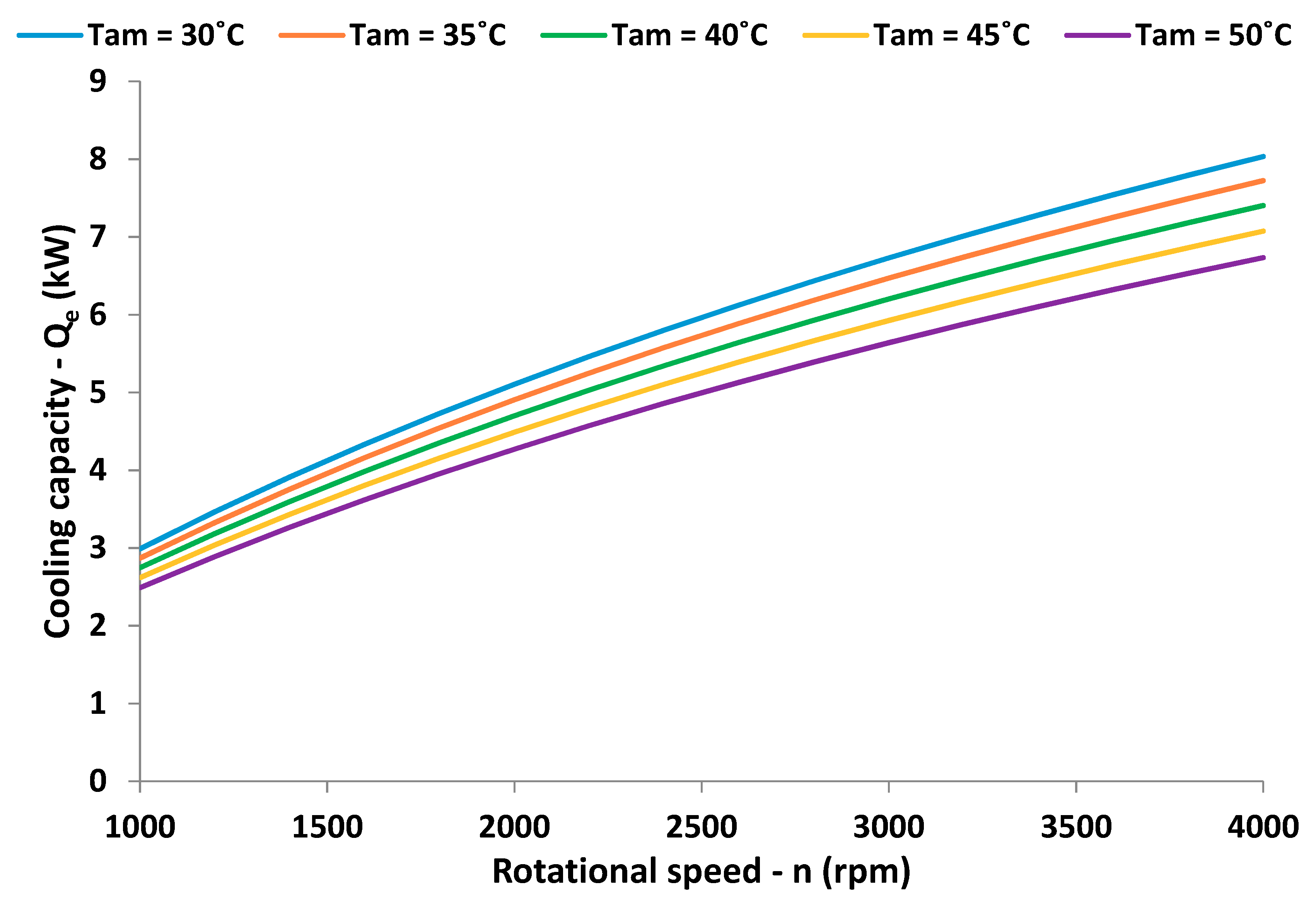
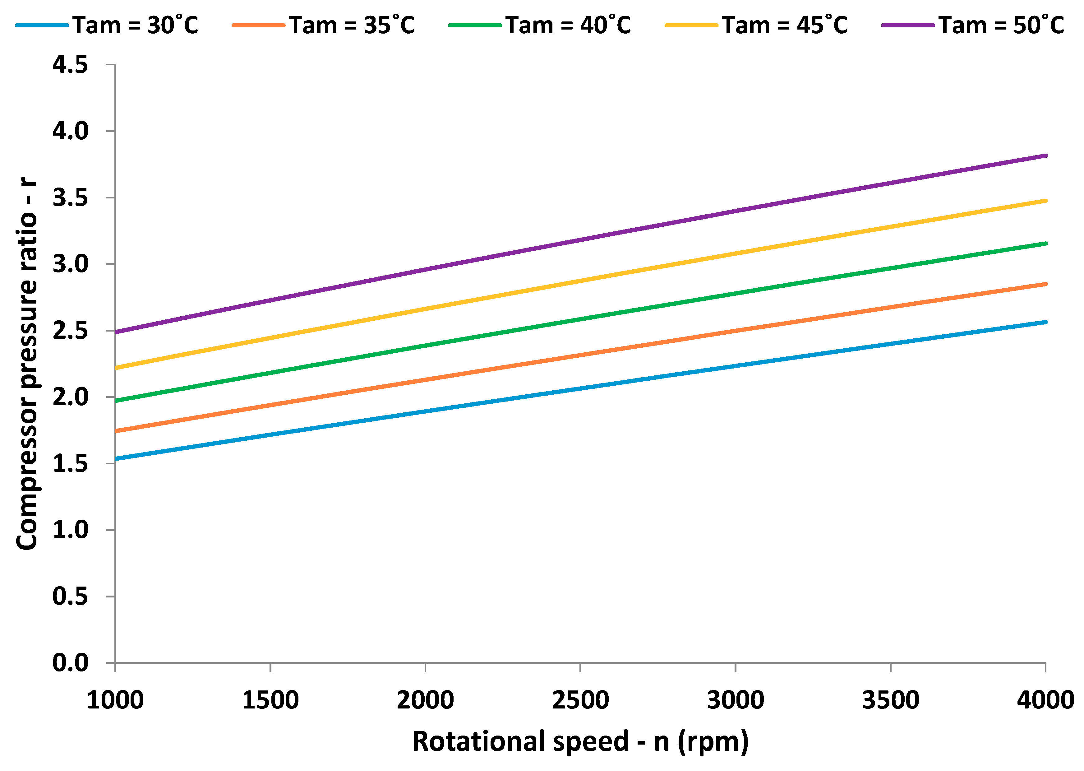
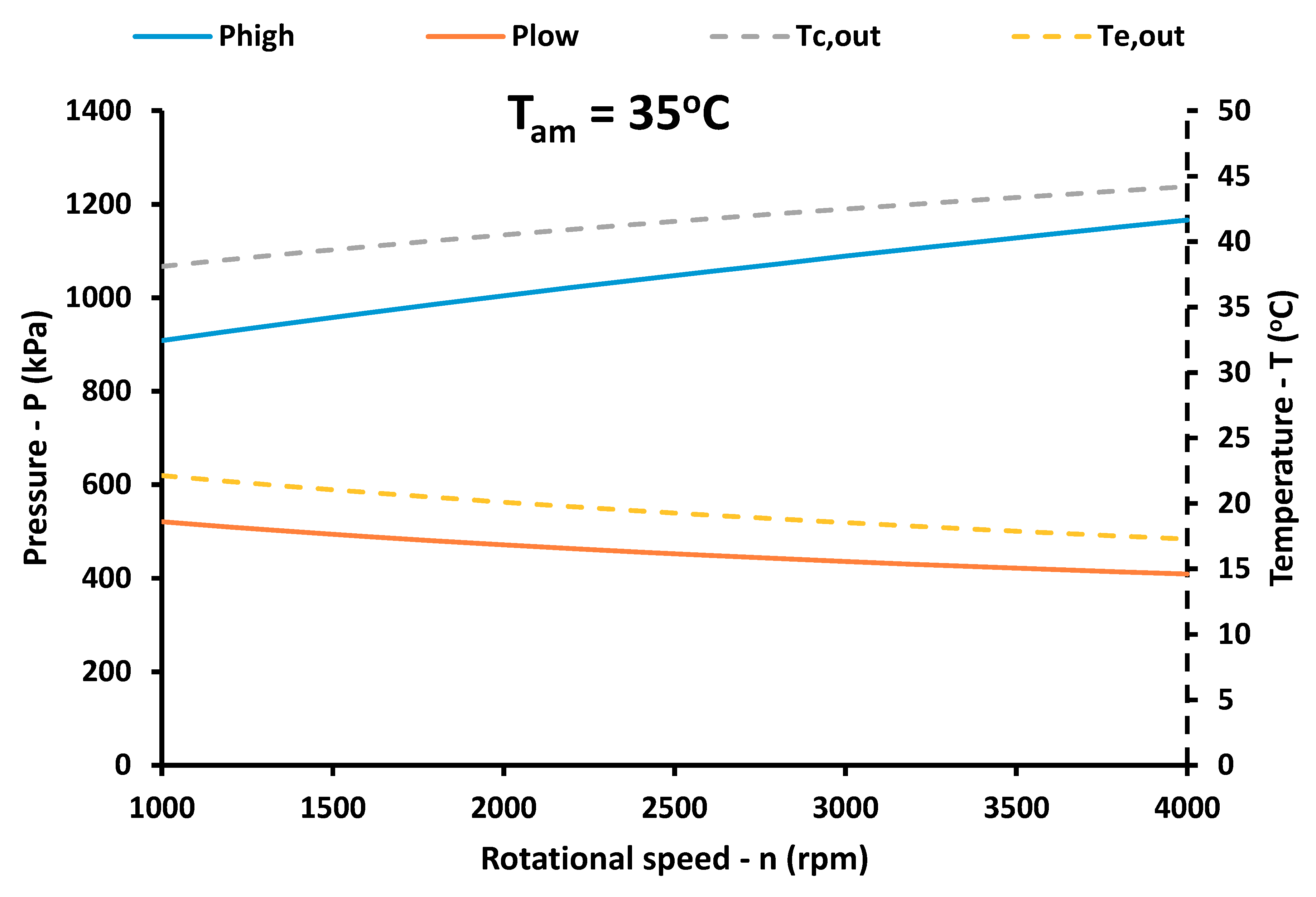
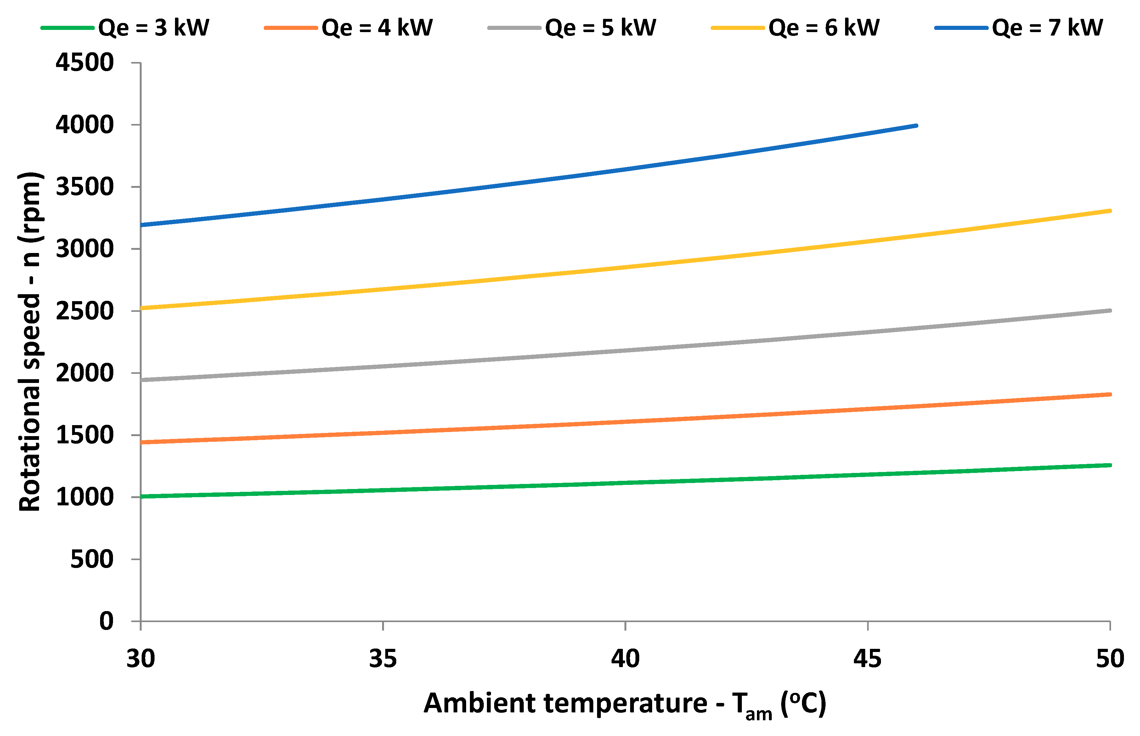
3.1. Impact of the Rotational Speed on the Performance

The first step in this work is the investigation of the impact of the rotational speed on the system performance. The indoor temperature is assumed to be 25 °C, while the ambient temperature is ranged from 30 °C up to 50 °C. It is important to state that the rotational speed is studied in the range of 1000 rpm to 4000 rpm with the value of 2000 rpm to be the nominal one. Figure 2 illustrates the COP for different rotational speeds and ambient temperatures. It is obvious that higher rotational speeds lead to lower COP. Moreover, the increase of the ambient temperature leads to a lower COP. It can be said that the impact of the rotational speed on the COP is more intense in the region between 1000 rpm and 2000 rpm. Figure 3 depicts the impact of the previous parameters on the cooling capacity. The increase of the rotational speed has a positive impact on the cooling capacity and the curves increases with a decreasing rate. Moreover, the cooling capacity is lower for higher ambient temperatures. Therefore, it can be said that both COP and cooling capacity are higher in low ambient temperatures, something that is reasonable. More specifically, in lower ambient temperatures, the condenser temperature is lower and so there is a higher potential for increased COP, according to the Carnot efficiency. Moreover, the system can reject higher amounts to the ambient and this fact gives the potential for higher cooling capacity. The interesting result is that the increase of the rotational speed leads to higher cooling capacity but to lower COP.

Figure 4 shows the pressure ratio in the compressor for the different cases. The increase of the ambient temperature leads to a higher condenser temperature and so the pressure ratio increases. Moreover, the increase of the rotational speed leads to a decrease in the evaporator temperature and increase in the condenser temperature in order for the system to operate properly. The respective results for the pressure levels and the outlet stream temperature levels are given in Figure 5 for a typical case with T_amb = 35 °C. More specifically, Figure 5 indicates that the increase of the rotational speed leads to higher condenser pressure level, lower evaporator pressure level, higher outlet air temperature from the condenser, and lower outlet air temperature from the evaporator.

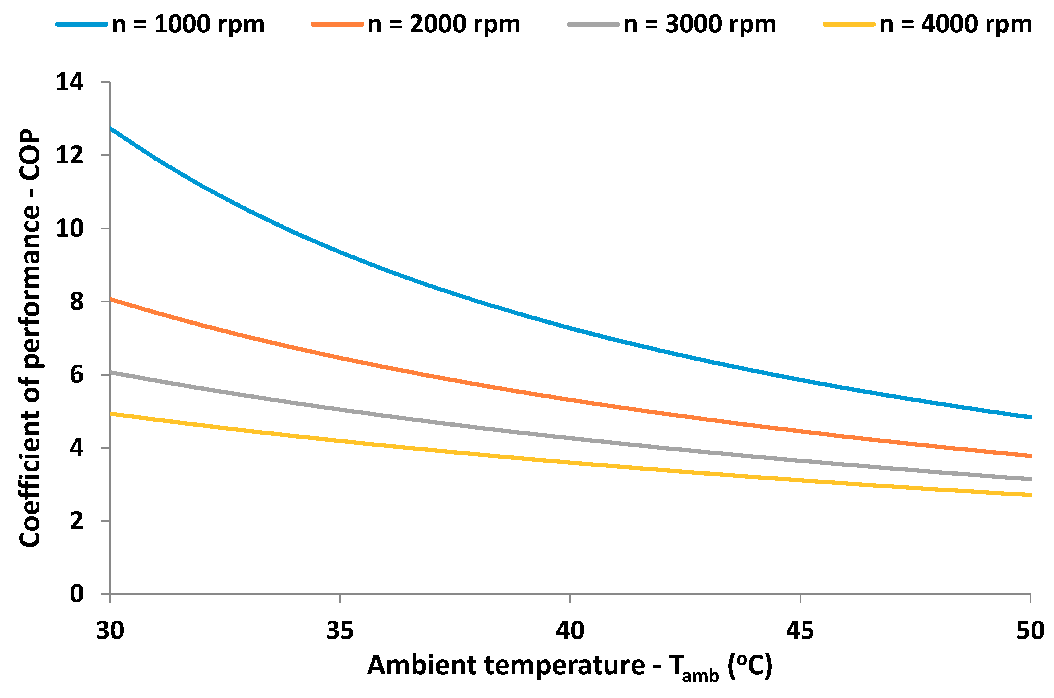
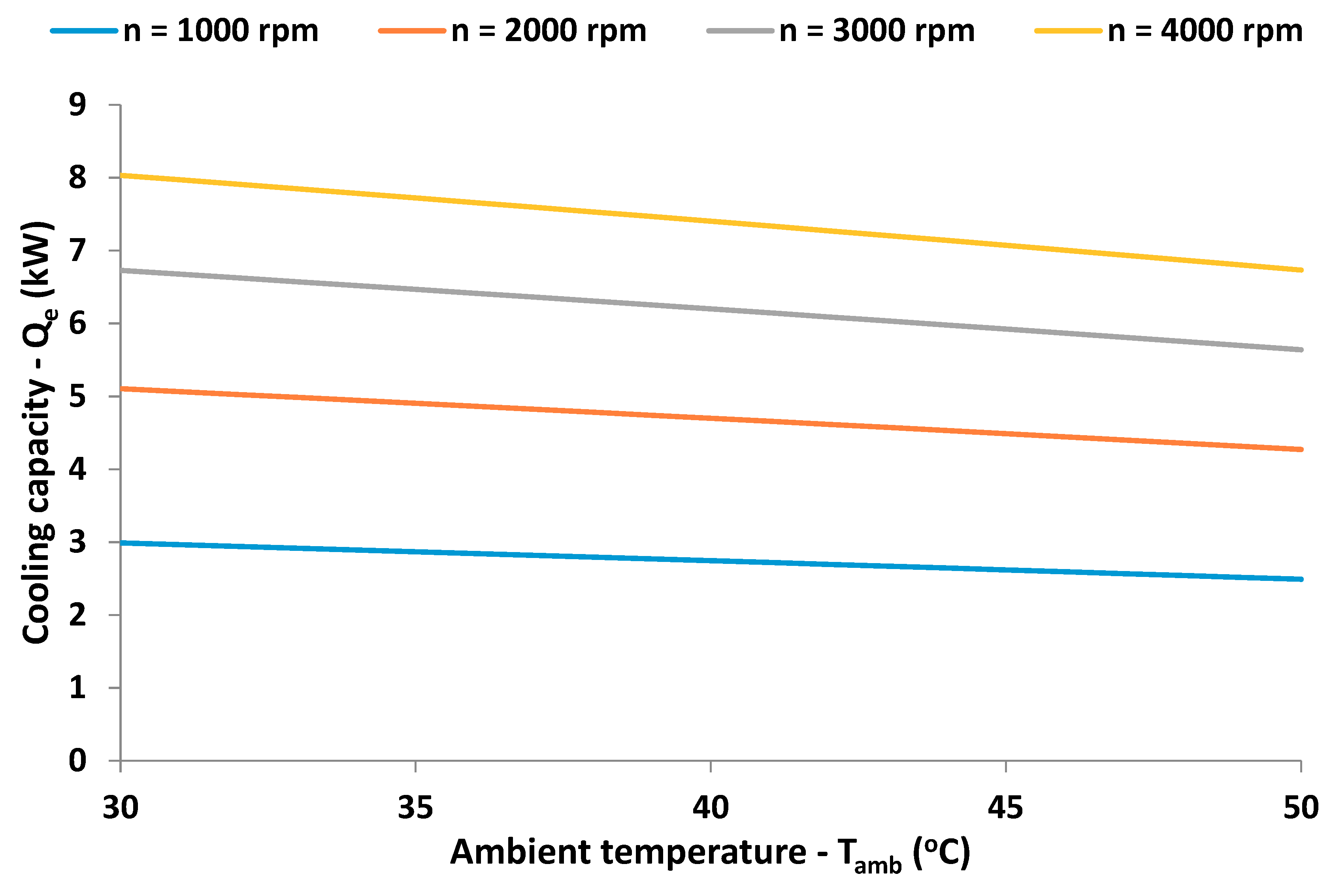
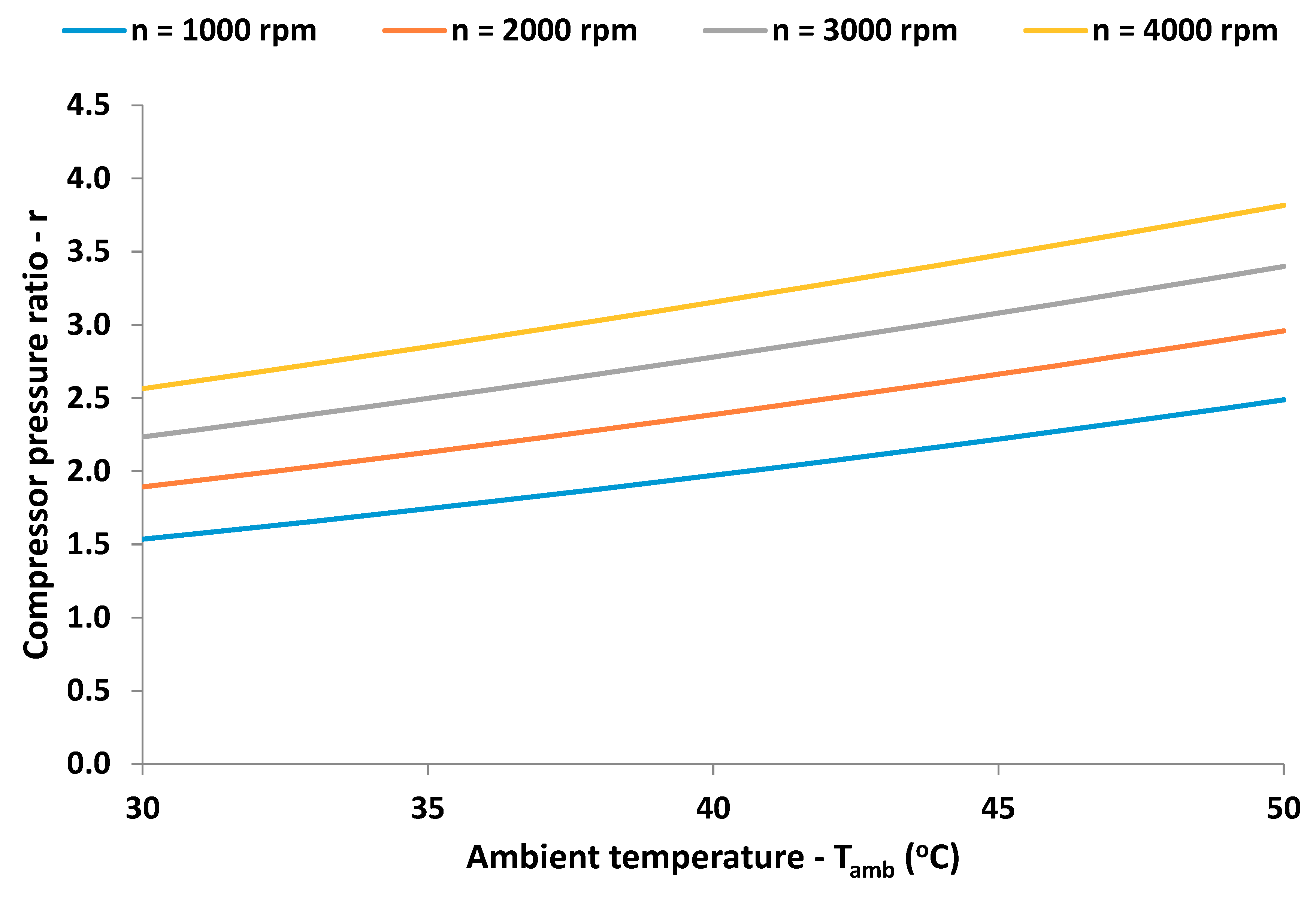
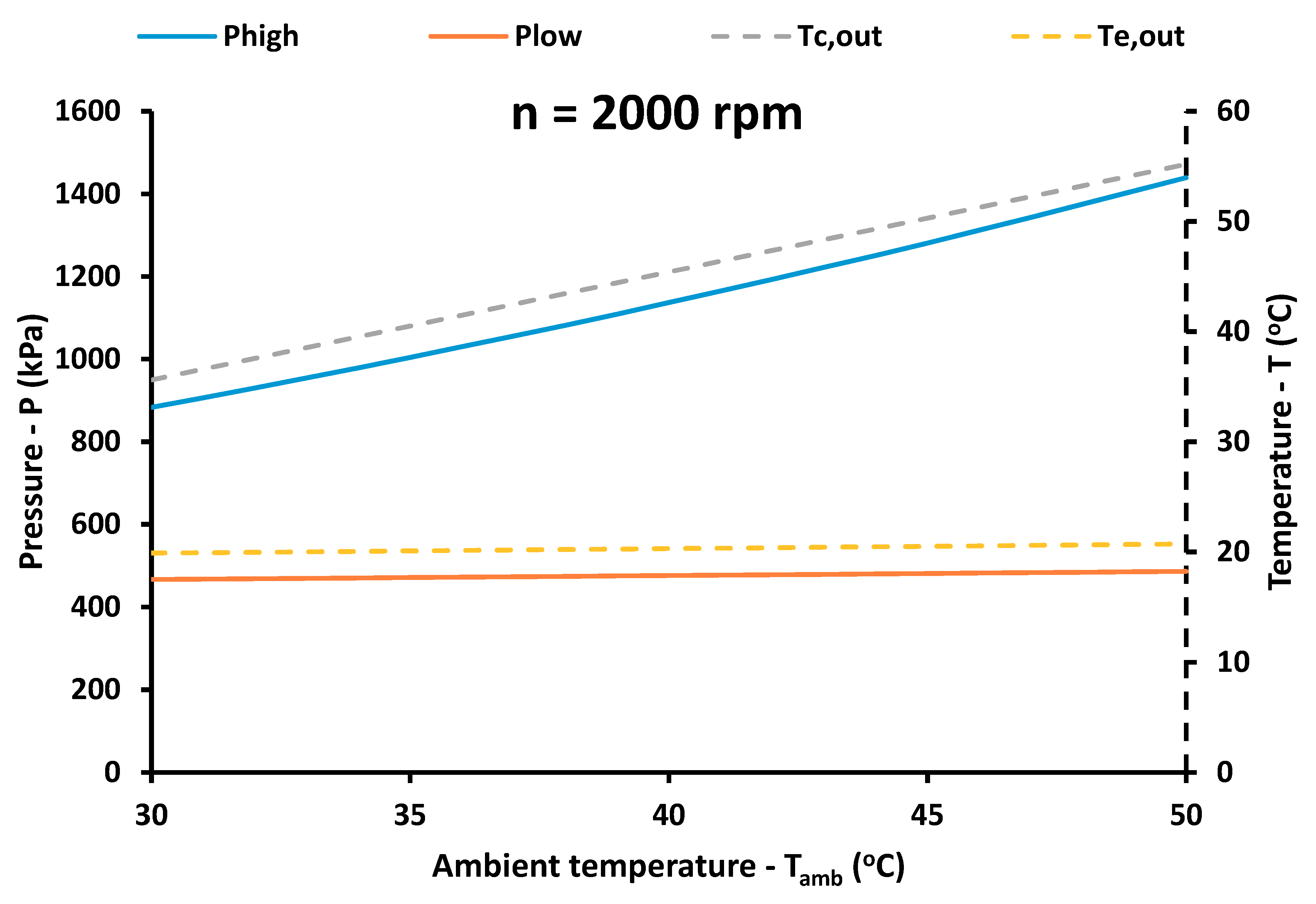
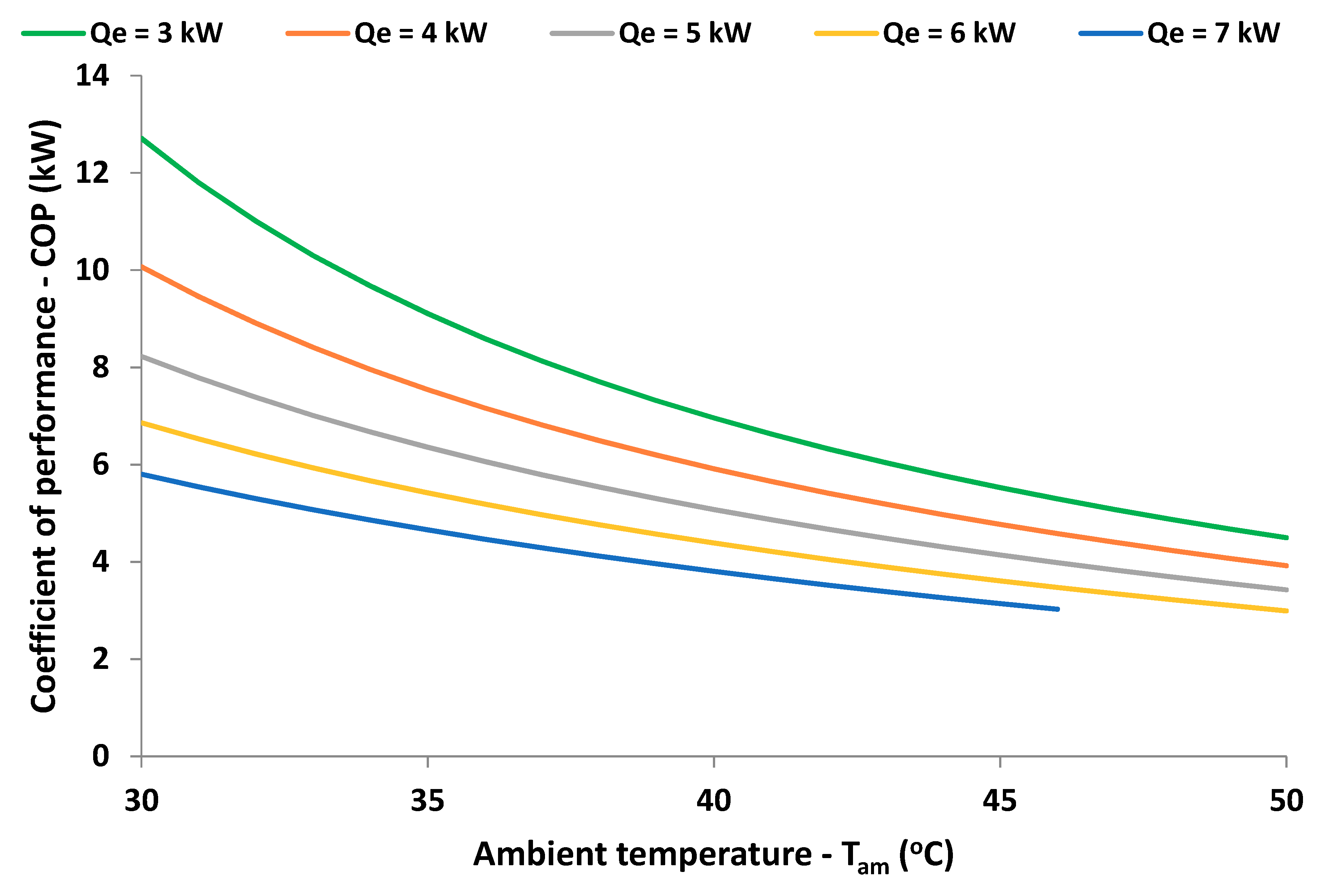
3.2. Impact of the Ambient Temperature on the Performance

The impact of the ambient temperature is highlighted in Section 3.2. The results are given for different rotational speeds (1000 rpm, 2000 rpm, 3000 rpm, and 4000 rpm), while the indoor temperature is T_ind = 25 °C. Figure 6 shows results about the COP and it can be said that the COP is lower for higher ambient temperatures and higher rotational speeds. Figure 7 shows that the cooling capacity presents a small decrease with the ambient temperature increase while it has an important increase with the increase of the rotational speeds. The conclusions from Figure 6 and Figure 7 are similar to the respective of Figure 2 and Figure 3, respectively.

Figure 8 shows that the pressure ratio is higher for higher ambient temperatures and rotational speeds. The increase of the ambient temperature leads to higher pressure levels in the condenser in order the heat rejection to the ambient to be possible. On the other hand, the low-pressure level in the evaporator is approximately the same for the different ambient temperatures, as the results of Figure 9 prove. It can be also said that the outlet air temperature from the condenser increase with the increase of the ambient temperature, while the outlet air temperature from the evaporator to the indoor space does not change with the ambient temperature variation. In other words, the examined system is able to provide the proper air temperature levels in the indoor space for all the ambient temperatures, but in the hotter days, the cooling capacity and the COP are decreased.

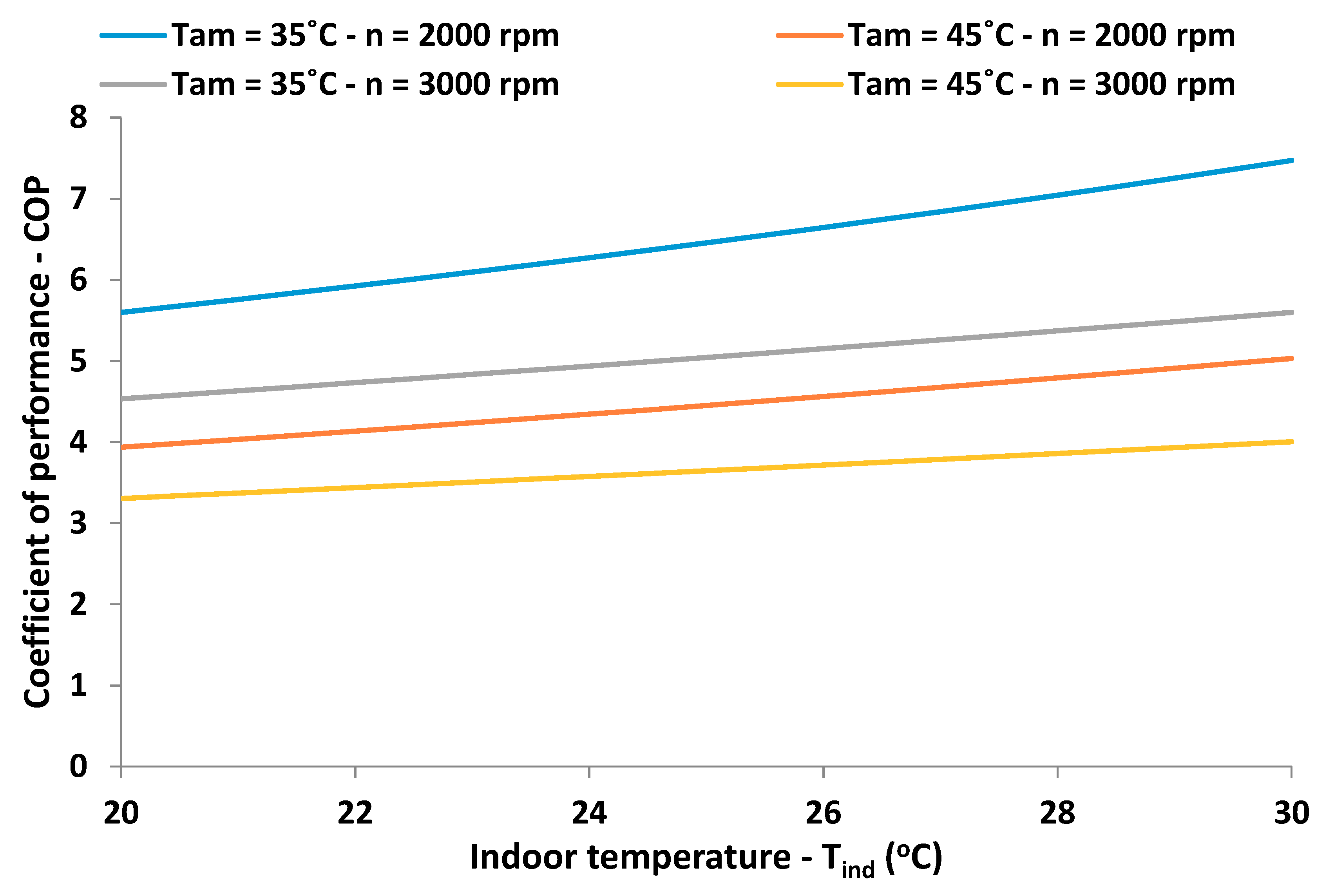
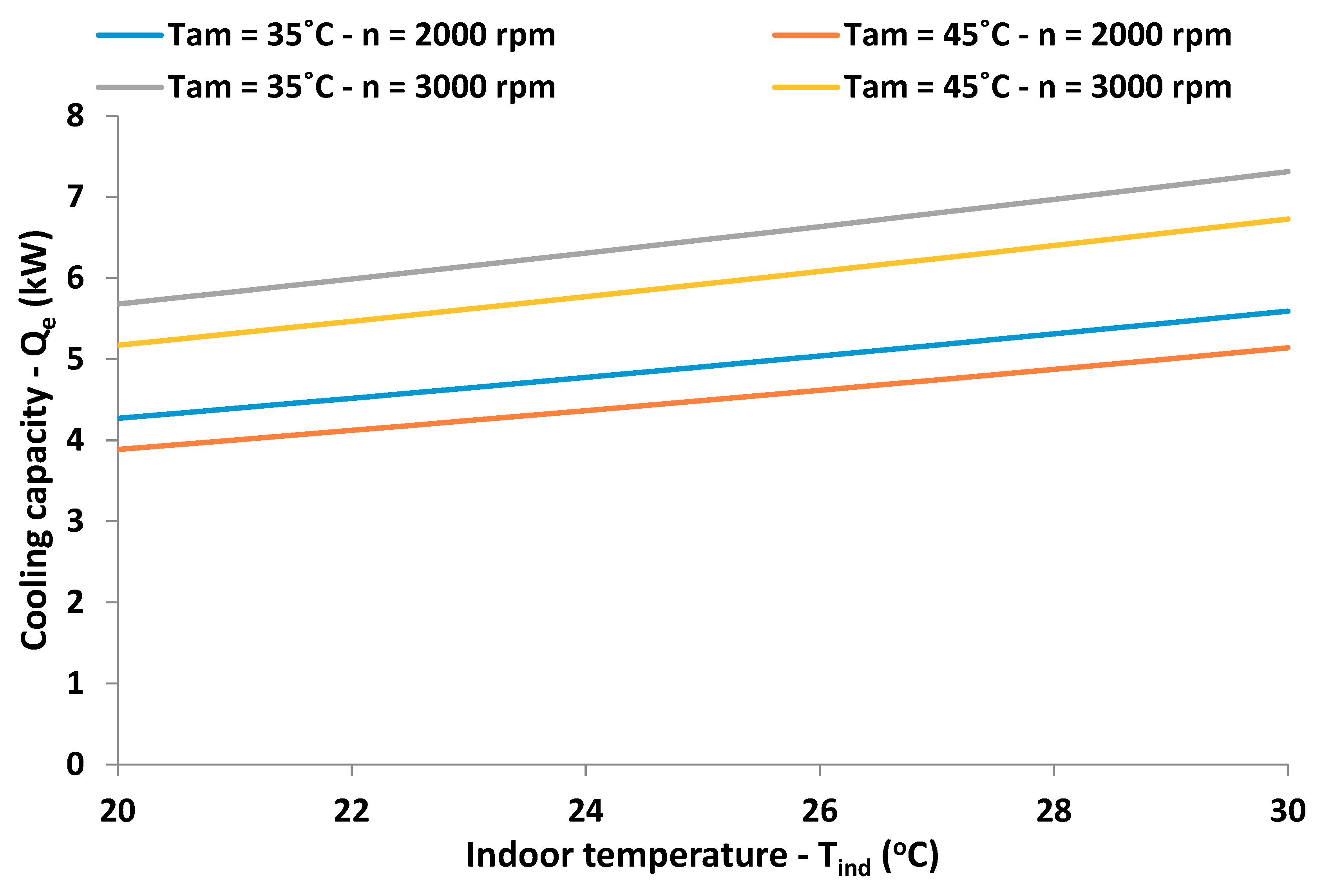
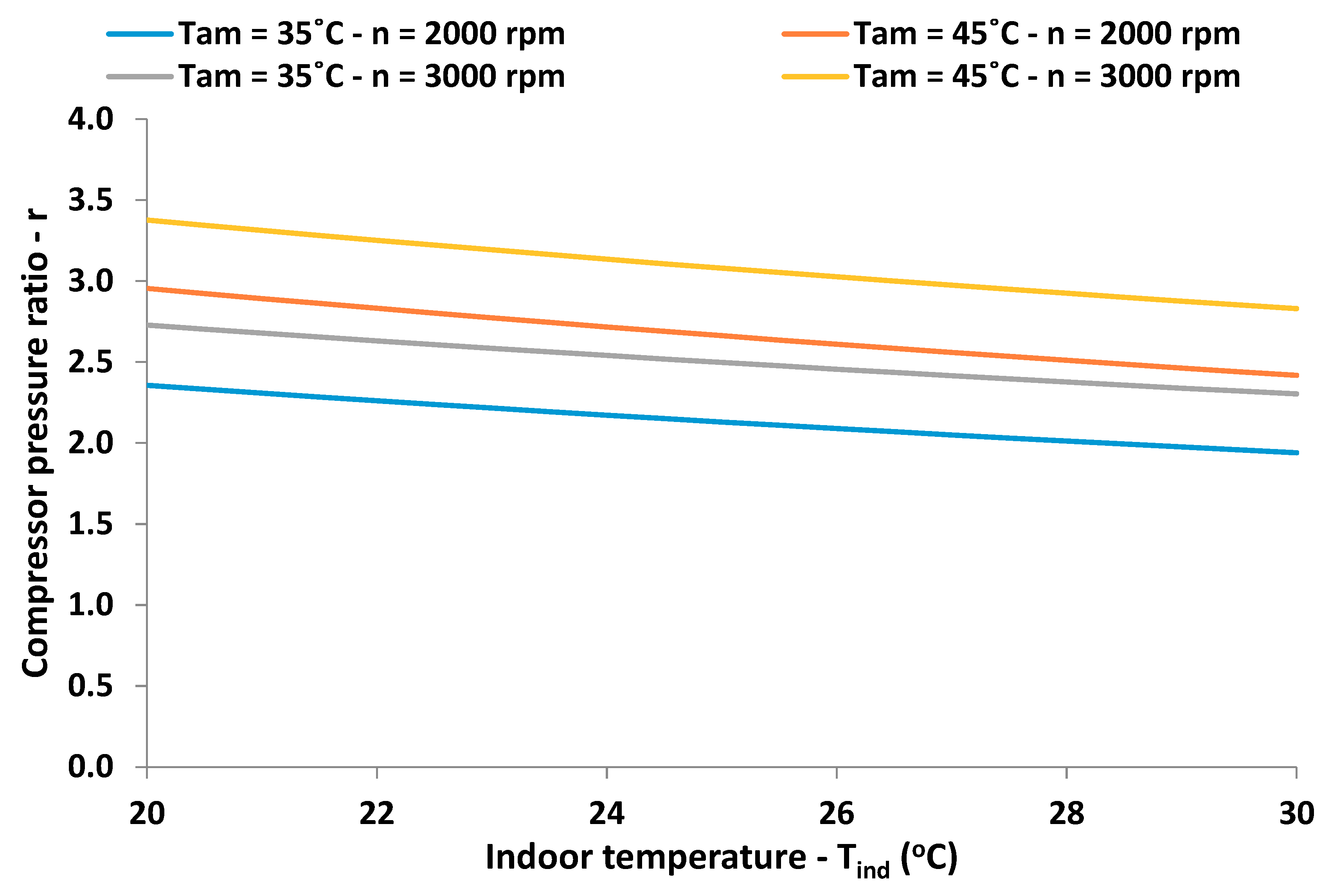
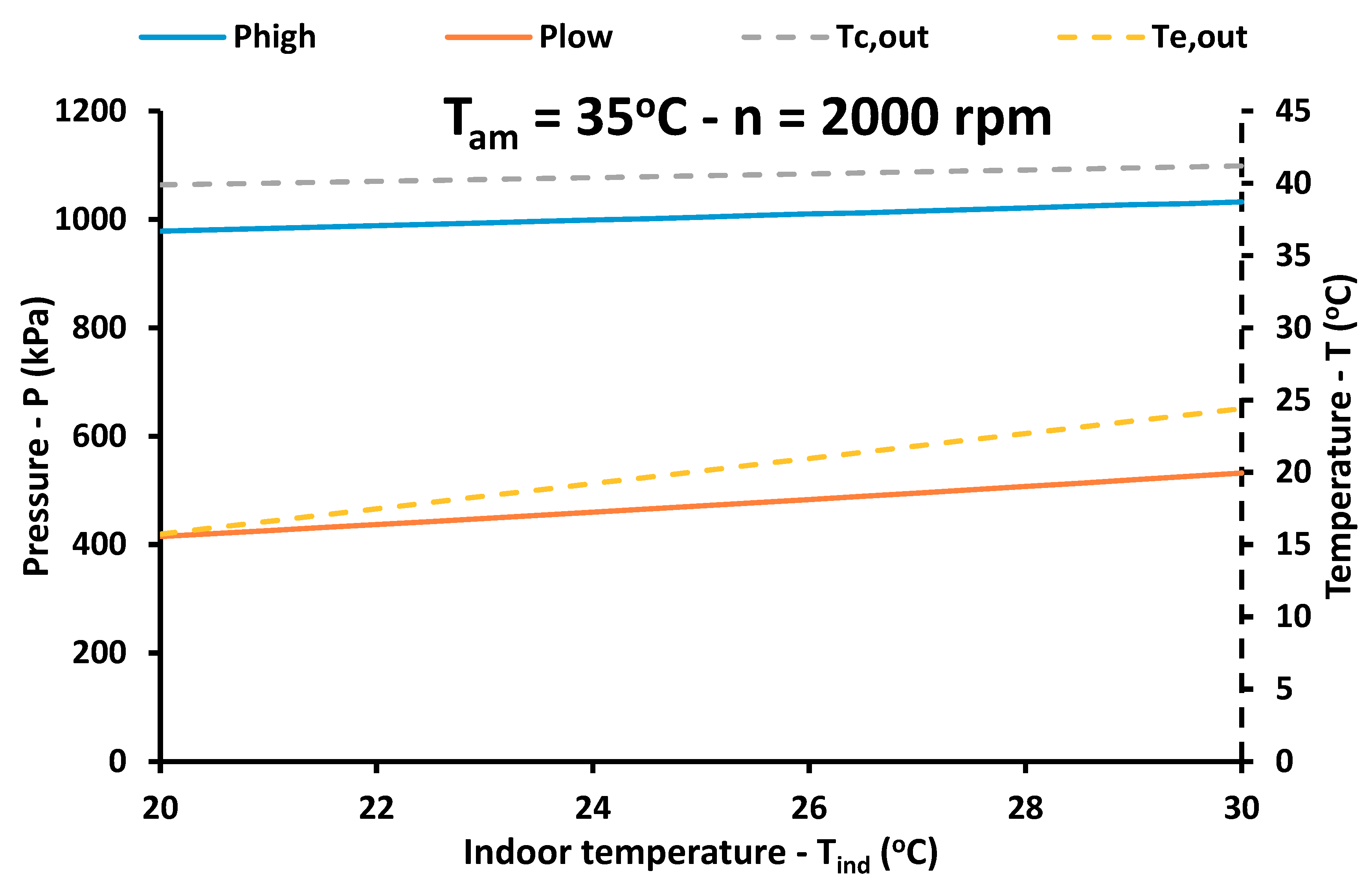
3.3. Impact of the Indoor Temperature on the Performance

The impact of the indoor air temperature is given in Figure 10, Figure 11, Figure 12 and Figure 13. The results are given for four operating scenarios: (T_am =35 °C − n = 2000 rpm, T_am = 45 °C – n = 2000 rpm, T_am = 35 °C – n = 3000 rpm and T_am = 45 °C – n = 3000 rpm). Figure 10 shows the COP for the investigated cases. It is obvious that higher indoor temperature leads to higher COP for all the operating scenario. Practically, higher indoor temperature makes the cooling production easier because the evaporator temperature can be relatively high for adequate cooling production. Moreover, Figure 11 illustrates that the increase in the indoor temperature leads to higher cooling capacity. Therefore, it can be said that in a case where the indoor temperature is 27 °C for example, then the heat pump is more efficient than the default case for operation at 25 °C. Figure 12 displays the pressure ratio in the compressor which has a decreasing rate with the indoor temperature increase. Practically, the higher indoor temperature increases the evaporator temperature and so the pressure ratio is lower. This fact can be verified by the results of Figure 13.

Figure 13 provides results for the case (T_am = 35 °C – n = 2000 rpm) and it indicates that the low pressure has an important increase with the indoor temperature increase. This result verifies the evaporator temperature increase. The air outlet temperature in the indoor space is also increased with the indoor temperature increase which is a reasonable result. The high pressure in the condenser and the air outlet temperature from the condenser present a small increase with the indoor temperature increase.

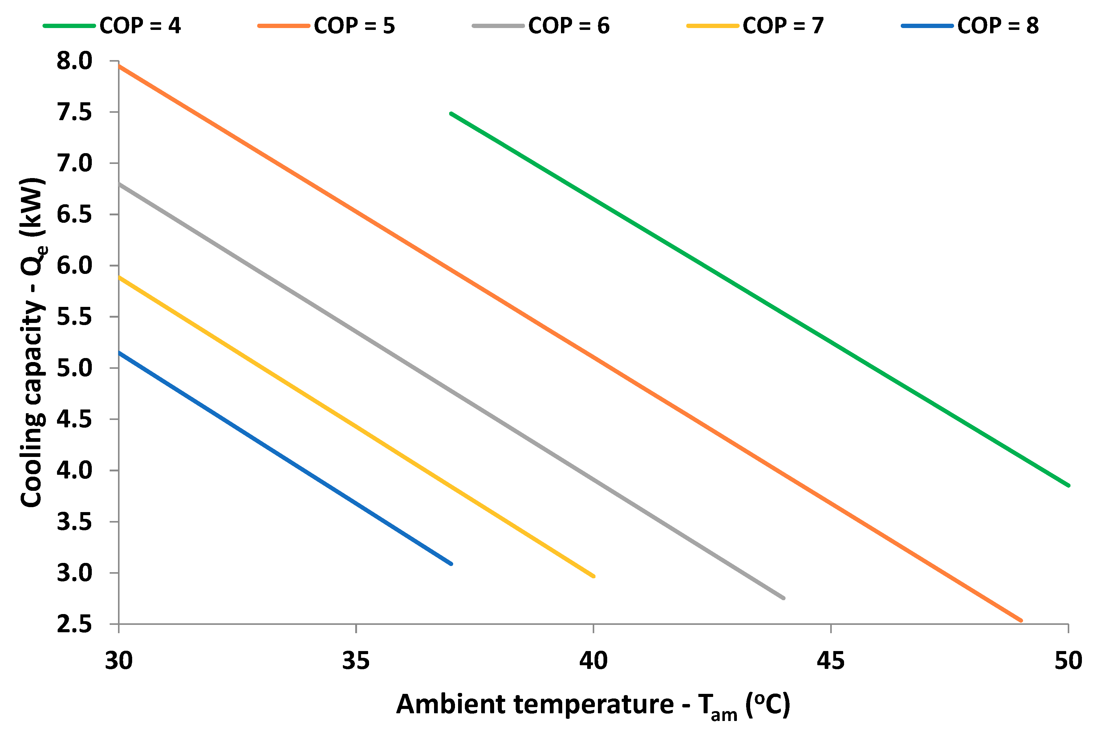
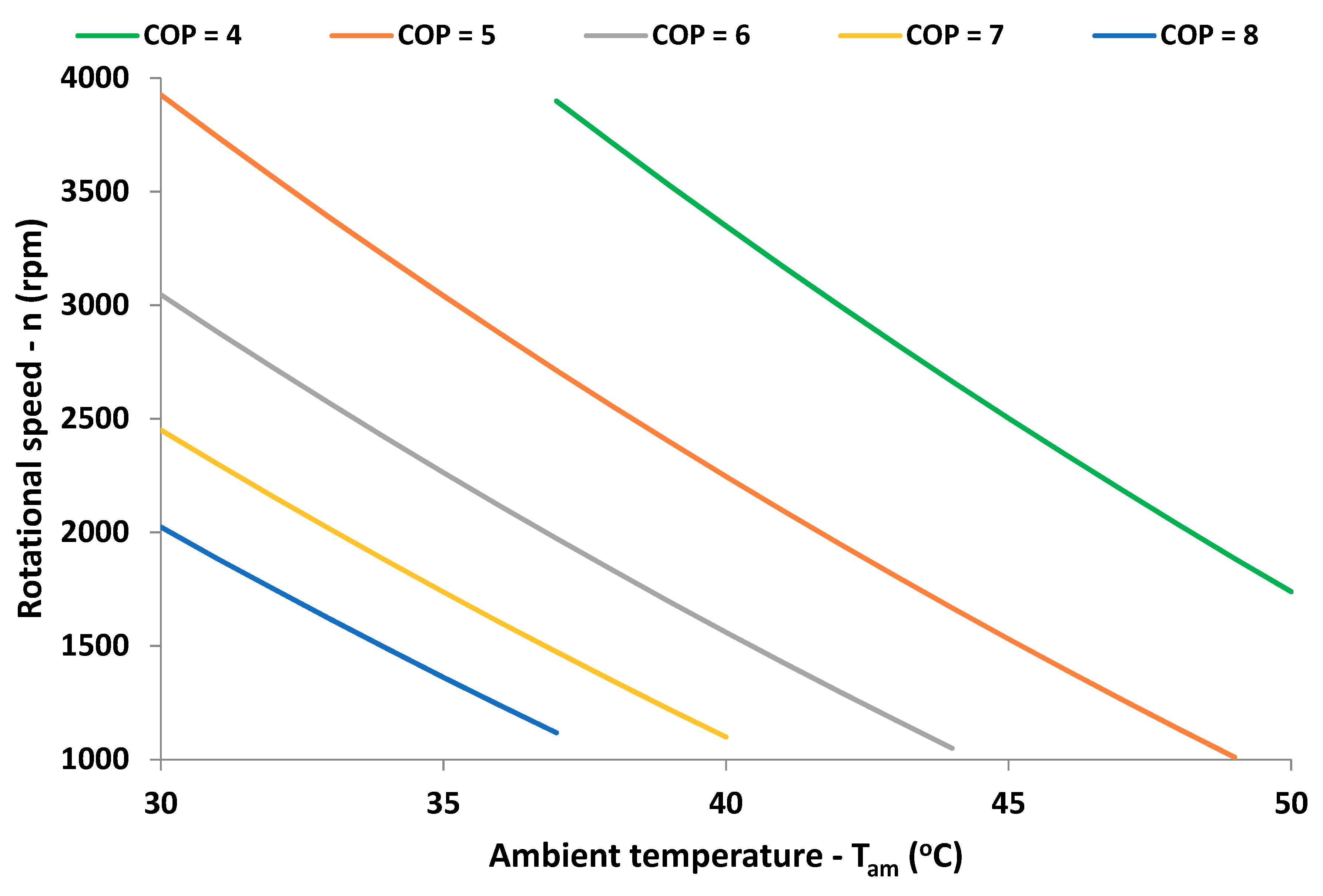
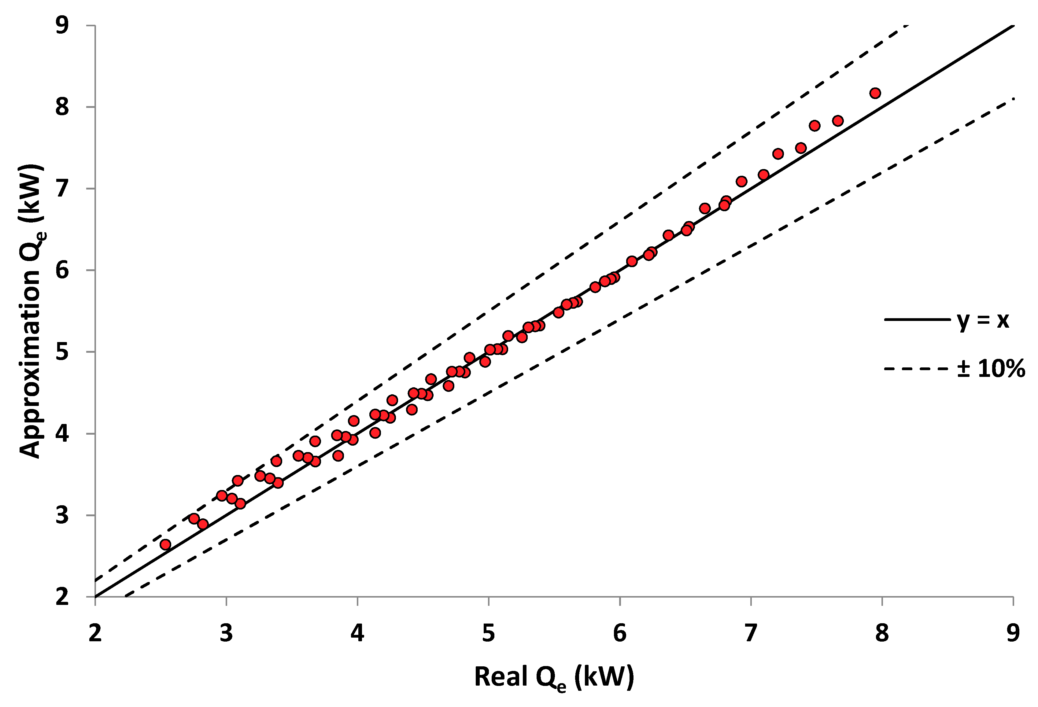
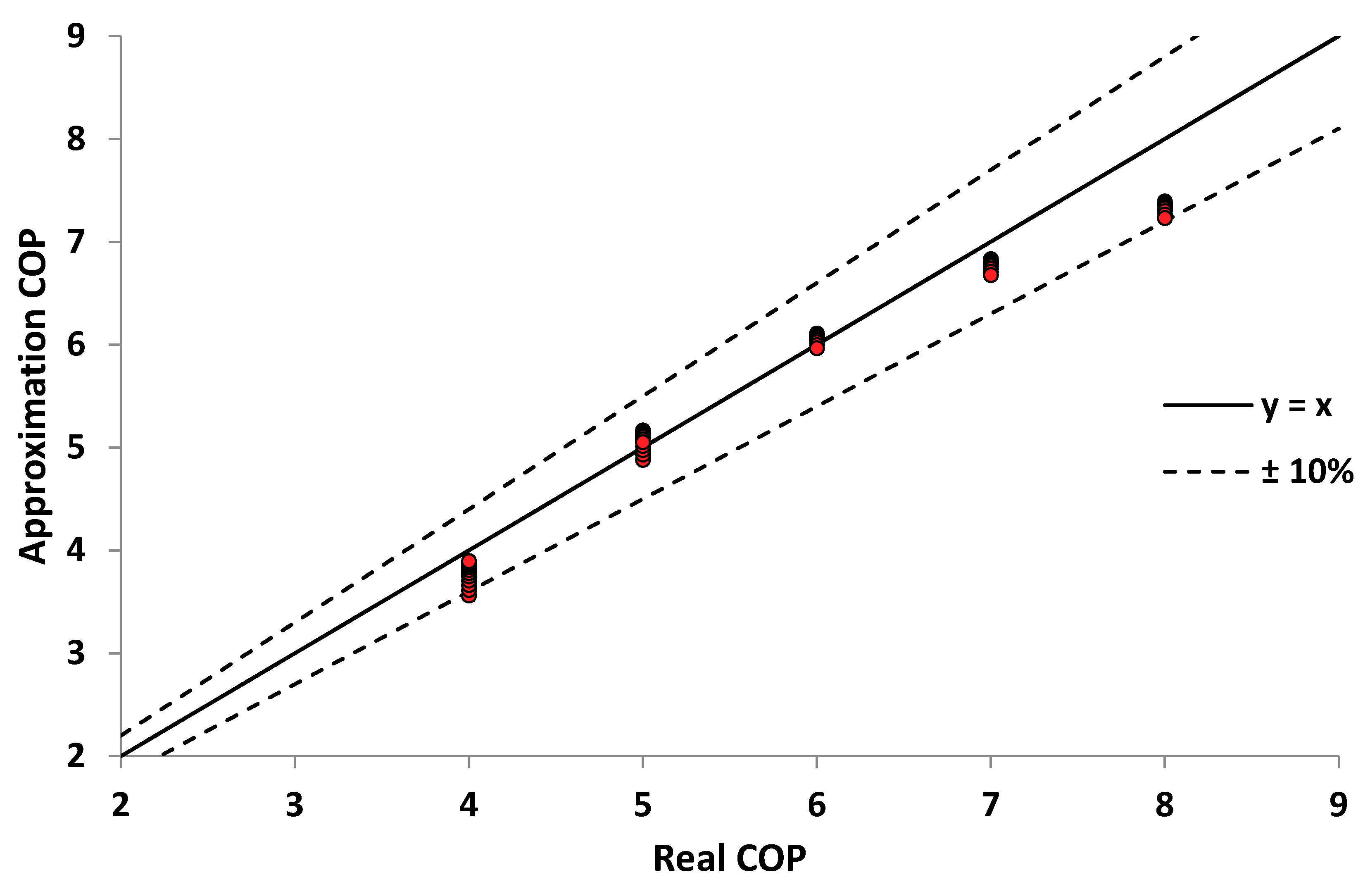
3.4. Deeper Analysis of the Examined Heat Pump

The previous section presented the impact of various parameters on the system performance and operation. This section presents results under some special cases with constant cooling capacity or constant COP. The rotational speed is adjusted in every case in order to achieve the demanded goal. The rotational speed is restricted in the range of 1000 rpm up to 4000 rpm.

Figure 14 and Figure 15 give the system performance for cases with constant cooling capacity. Practically, Figure 14 shows the COP for different cooling capacities and ambient temperatures. The useful result is that the COP is lower when the cooling capacity increases. Figure 15 proves that the rotational speed increases when the cooling capacity is higher and when the ambient temperature is also higher. Practically, the rotational speed is higher in the cases with greater needs in the system. It has also to be said that the curves of Q_e = 7 kW in Figure 14 and Figure 15 are shorter than the other curves due to restriction in the rotational speed (up to 4000 rpm).

Figure 16 and Figure 17 correspond to the cases with constant COP. Figure 16 shows that the cooling capacity has a linear decrease with the ambient temperature increases and it is higher for the cases with lower COP. Figure 17 shows that the rotational speeds are lower when the ambient temperature increases. This is an interesting result and it is explained by the decrease in the cooling capacity, when the ambient temperature increases and the COP is constant, the fact that leads to lower rotation speed. Therefore, it can be said that the critical parameter in the rotational speed adjustment is the cooling load value.

The next step in this work is the deeper investigation of the system performance. For this reason, the operating scenarios of Figure 16 and Figure 17, under constant COP, are examined mathematically in order to develop proper correlations. Equation (18) correlates the cooling capacity with the rotational speed and the ambient temperature, while the equation correlates the COP with the same parameters. These equations are expressed with dimensionless parameters using the nominal operating case (see Table 2 for the exact values) in order to create more general conclusions. The accuracy of these equations is higher with R² equal to 99.19% for Equation (18) and 96.47% for Equation (19).

• Cooling capacity correlation (R² = 99.19%)

  $$\frac{Q_e}{Q_{e,0}}=1+0.637445\cdot \left(\frac{n-n_0}{n_0}\right)-0.3647\cdot \left(\frac{T_{am}-T_{am,0}}{T_{am,0}}\right)$$

  (18)
• COP correlation (R² = 96.47%)

  $$\frac{COP}{CO{P}_0}=1-0.40875\cdot \left(\frac{n-n_0}{n_0}\right)-1.04965\cdot \left(\frac{T_{am}-T_{am,0}}{T_{am,0}}\right)$$

  (19)

The previous equations are valid for the following restrictions:

(a)

$-0.5<\frac{n-n_0}{n_0}<1.0$

(b)

$-0.1429<\frac{T_{am}-T_{am,0}}{T_{am,0}}<0.4286$

Figure 18 and Figure 19 show the validity of the suggested equations by plotting the approximation values using the equations and the real values from the model. It is obvious that the maximum errors are up to 10% with the mean error in the cooling capacity to be 2.17% and in the COP 3.17%.

Equation (18) shows that the cooling capacity increases with the increase of the rotational speed, while it decreases with the increase of the ambient temperature. The factor of the ambient temperature term is 0.3647 and it is smaller than the factor of the rotational speed which is 0.637445. This result proves that the rotational speed has a higher impact on the cooling capacity than the ambient temperature. This conclusion is verified by the curves slope in Figure 3 and Figure 7.

Equation (19) shows that the COP decreases with the increase of the rotational speed and with the ambient temperature increase. The factor for the rotational speed is 0.40875 and for the ambient temperature is 1.04965. These results indicate that the ambient temperature has a higher impact on the COP than the rotational speed. These conclusions are verified by the curves slope in Figure 2 and Figure 6.

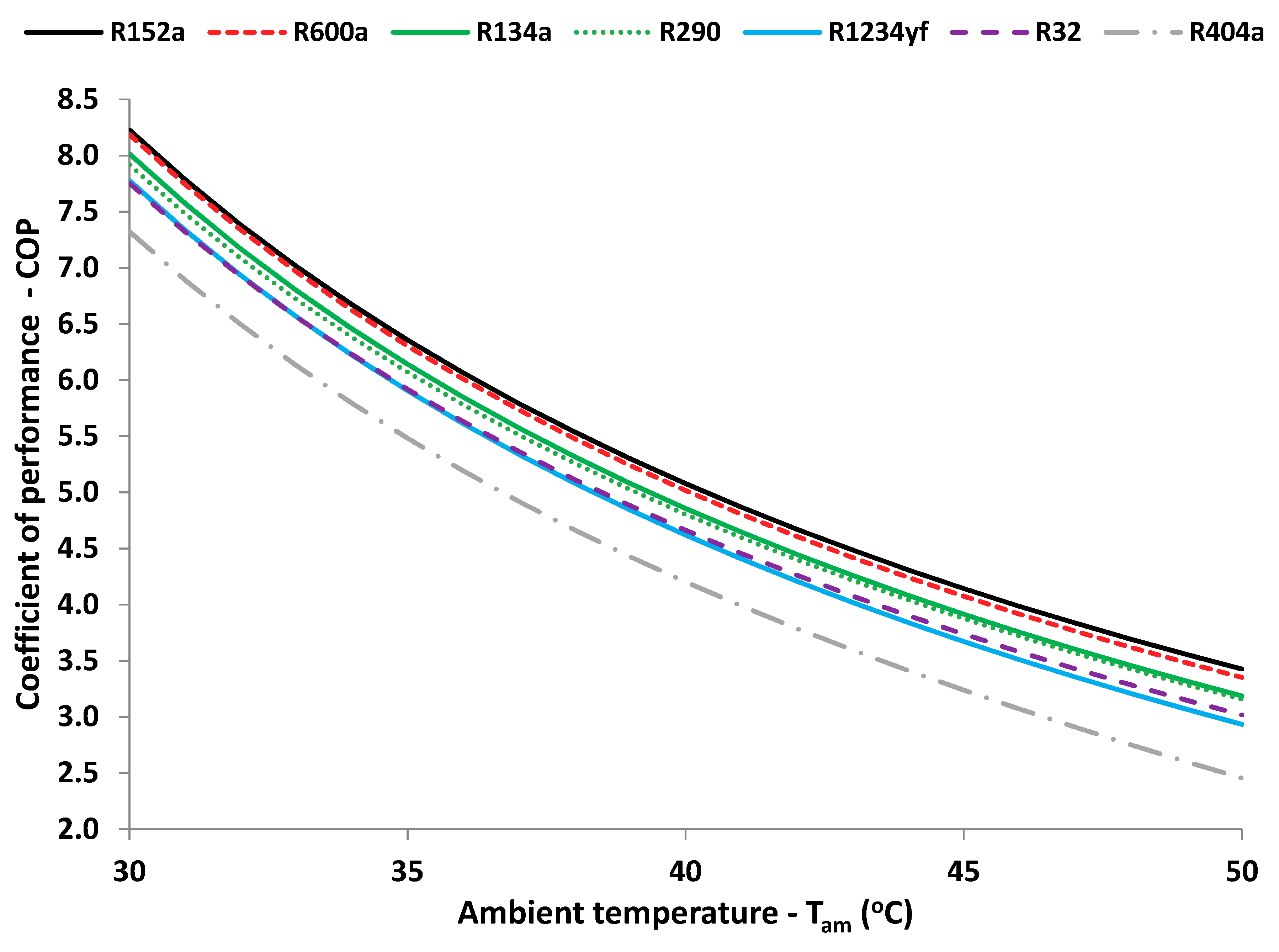
3.5. Comparative Study with Other Refrigerants

The last step in this work is the comparison of the R152a with other refrigerants. The R152a is compared with the natural refrigerants R600a and R290, with the harmful refrigerants R134a and R404a, as well as with the promising refrigerants R32 and R1234yf. Figure 20 and

Table 4. Comparison of the different working fluids with R152a for Q_e = 5 kW and T_ind = 25 °C.

Tamb (°C)	COP
	R152a	R600a	R134a	R290	R1234yf	R32	R404a
30	8.227	8.186	8.014	7.916	7.776	7.752	7.322
31	7.786	7.742	7.573	7.481	7.336	7.32	6.89
32	7.383	7.337	7.169	7.083	6.933	6.925	6.495
33	7.012	6.964	6.798	6.718	6.563	6.562	6.13
34	6.671	6.621	6.456	6.381	6.221	6.228	5.794
35	6.356	6.303	6.140	6.07	5.905	5.918	5.482
36	6.064	6.009	5.847	5.781	5.612	5.631	5.192
37	5.791	5.735	5.574	5.511	5.338	5.364	4.92
38	5.538	5.479	5.319	5.26	5.083	5.114	4.666
39	5.300	5.240	5.080	5.025	4.843	4.881	4.427
40	5.078	5.016	4.856	4.804	4.619	4.662	4.202
41	4.868	4.805	4.646	4.597	4.407	4.455	3.989
42	4.671	4.607	4.447	4.401	4.208	4.261	3.787
43	4.486	4.419	4.26	4.216	4.019	4.077	3.596
44	4.310	4.242	4.082	4.041	3.84	3.902	3.413
45	4.143	4.074	3.914	3.875	3.67	3.737	3.238
46	3.985	3.915	3.754	3.718	3.509	3.579	3.07
47	3.835	3.764	3.602	3.568	3.355	3.429	2.908
48	3.692	3.62	3.457	3.425	3.208	3.286	2.752
49	3.556	3.482	3.319	3.288	3.068	3.149	2.601
50	3.426	3.351	3.187	3.157	2.933	3.017	2.454
Mean COP	5.342	5.2815	5.119	5.063	4.8784	4.917	4.444
Enhancement		1.14%	4.36%	5.51%	9.50%	8.65%	20.20%

give the comparative results. These results are given to different ambient temperatures and for cooling production equal to 5 kW. The rotational speed is different among the examined cases in order to achieve this cooling capacity. Moreover, it has to be said that the indoor temperature has the default value of 25 °C.

It is found that the R152a has the highest COP among the examined cases, which makes it a promising working fluid in the heat pumps. For all the ambient temperatures, the R152a has the highest performance, with the R600a to be the second case and the R404a to be the worst working fluid. The mean enhancement in the COP with the R152a is 1.14% compared to the R600a, while it is 4.36%, 5.51%, 9.50%, 8.65% and 20.20% compared to R134a, R290, R1234yf, and R404a respectively. At this point, it can be said that the found results are in accordance to the literature because the studies [12,13,14] have found the R152a to be more efficient than other refrigerants such as R134a and R32.

Therefore, it can be said that the R152a has great potential as a working fluid by the energetic point of view. Taking into consideration is relatively low GWP = 138 which is lower than 150, the R152a can be a choice for the future of the cooling systems. The medium flammability problems have to be taken into consideration for safety reasons and these are the only limitations of this refrigerant. Lastly, it has to be stated that the COP values are relatively high in low ambient temperatures and this fact indicates that the examined system is a highly efficient air conditioner.

About the future studies, the R152a refrigeration system can be examined in a dynamic model coupled with a building with real cooling loads. A more detailed model is used to be developed. Also, stochastic, adaptive, and dynamic control techniques [35,36] can be applied for the proper optimization of the overall configuration.

4. Conclusions

The objective of this paper is the detailed investigation of a heat pump operating with the environmentally friendly refrigerant, the R152a. The analysis is conducted with a developed model in EES which is validated with literature data. The system is examined parametrically and regression models for its performance are suggested. The most important conclusions of this work are summarized below:

-

In the nominal operating conditions, the examined heat pump has 5 kW cooling capacity and a COP equal to 6.46.

-

The increase of the rotational speed leads to higher cooling capacity and to lower COP.

-

The increase of the ambient temperature leads to lower cooling capacity and to lower COP.

-

The increase of the indoor temperature leads to higher cooling capacity and to higher COP.

-

It is found that the rotational speed is the most important parameter for the cooling capacity value, while the ambient temperature is the most important parameter for the COP value.

-

The R152a is found to be the most efficient refrigerant compared to six other refrigerants. The mean enhancement with the R600a is found to be 1.14%, while with R134a 4.36%, while with the R404a 20.20%.

-

The final results of this work can be utilized for the proper modeling of a cooling system with a heat pump with R152a. The developed models can be utilized for the simulation of this system in different operating conditions. Moreover, the advantages of the R152a are discussed and explained in this work and finally, this refrigerant is suggested as a reliable choice.

To conclude, the refrigerant R152a is a highly effective choice for the cooling vapor compression cycles. This refrigerant is non-toxic and it has a low GWP, while it has a reasonable cost. The only issue is the increased flammability which is not so great. All the factors can make this refrigerant a reliable choice for future cooling systems.

References

1. Ciconkov, R. Refrigerants. There is still no vision for sustainable solutions. Int. J. Refrig. 2018, 86, 441–448. [Google Scholar] [CrossRef]
2. Khanmohammadi, S.; Goodarzi, M.; Khanmohammadi, S.; Ganjehsarabi, H. Thermoeconomic modeling and multi-objective evolutionary-based optimization of a modified transcritical CO2 refrigeration cycle. Therm. Sci. Eng. Prog. 2018, 5, 86–96. [Google Scholar] [CrossRef]
3. Piccolo, A.; Siclari, R.; Rando, F.; Cannistraro, M. Comparative Performance of Thermoacoustic Heat Exchangers with Different Pore Geomeyries in Oscillatory Flow Implementation of Experimental Techniques. Appl. Sci. 2017, 2, 784. [Google Scholar] [CrossRef]
4. Cannistraro, M.; Mainardi, E.; Bottarelli, M. Testing a Dual-Source Heat Pump. Math. Model. Eng. Probl. 2018, 5, 197–204. [Google Scholar] [CrossRef]
5. Regulation, EU No 517/2014 of the European Parliament and the Council of 16 April 2014 on Fluorinated Greenhouse Gases and Repealing Regulation (EC) No 842/2006. Available online: http//www.eea.europa.eu/policy-documents/regulation-eu-no-517-2014 (accessed on 30 December 2018).
6. IPCC. Climate Change 2013, The Physical Science Basis. Contribution of Working Group I to the Fifth Assessment Report of the Intergovernmental Panel on Climate Change, 1st ed.; Cambridge University Press: New York, NY, USA, 2013. [Google Scholar]
7. Abas, N.; Kalair, A.R.; Khan, N.; Haider, A.; Saleem, Z.; Saleem, M.S. Natural and synthetic refrigerants, global warming, A review. Renew. Sustain. Energy Rev. 2018, 90, 557–569. [Google Scholar] [CrossRef]
8. Available online: https//en.wikipedia.org/wiki/List_of_refrigerants (accessed on 5 November 2018).
9. McLinden, M.; Steven Brown, J.; Brignoli, R.; Kazakov, A.; Domanski, P. Limited options for low-global-warming-potential refrigerants. Nat. Commun. 2017, 8, 14476. [Google Scholar] [CrossRef] [Green Version]
10. Tsamos, K.M.; Ge, Y.T.; Santosa, I.; Tassou, S.A.; Bianchi, G.; Mylona, Z. Energy analysis of alternative CO2 refrigeration system configurations for retail food applications in moderate and warm climates. Energy Convers. Manag. 2017, 150, 822–829. [Google Scholar] [CrossRef]
11. Gullo, P.; Elmegaard, B.; Cortella, G. Energy and environmental performance assessment of R744 booster supermarket refrigeration systems operating in warm climates. Int. J. Refrig. 2016, 64, 61–79. [Google Scholar] [CrossRef] [Green Version]
12. Bolaji, B.O. Experimental study of R152a and R32 to replace R134a in a domestic refrigerator. Energy 2010, 35, 3793–3798. [Google Scholar] [CrossRef]
13. Nie, J.; Li, Z.; Kong, X.; Li, D. Analysis and Comparison Study on Different HFC Refrigerants for Space Heating Air Source Heat Pump in Rural Residential Buildings of North China. Procedia Eng. 2017, 205, 1201–1206. [Google Scholar] [CrossRef]
14. Cabello, R.; Sánchez, D.; Llopis, R.; Arauzo, I.; Torrella, E. Experimental comparison between R152a and R134a working in a refrigeration facility equipped with a hermetic compressor. Int. J. Refrig. 2015, 60, 92–105. [Google Scholar] [CrossRef] [Green Version]
15. Sanchez, D.; Cabello, R.; Llopis, R.; Arauzo, I.; Catalán-Gil, J.; Torrella, E. Energy performance evaluation of R1234yf, R1234ze(E), R600a, R290 and R152a as low-GWP R134a alternatives. Int. J. Refrig. 2017, 74, 269–282. [Google Scholar] [CrossRef] [Green Version]
16. Perez-Garcia, V.; Belman-Flores, J.N.; Rodríguez-Munoz, L.J.; Rangel-Hernandez, V.H.; Gallegos-Munoz, A. Second Law Analysis of a Mobile Air Conditioning System with Internal Heat Exchanger Using Low GWP Refrigerants. Entropy 2017, 19, 175. [Google Scholar] [CrossRef]
17. Cabello, R.; Sánchez, D.; Llopis, R.; Catalán, J.; Nebot-Andrés, L.; Torrella, E. Energy evaluation of R152a as drop in replacement for R134a in cascade refrigeration plants. Appl. Therm. Eng. 2017, 110, 972–984. [Google Scholar] [CrossRef] [Green Version]
18. Yang, W.-W.; Cao, X.-Q.; He, Y.-l.; Yan, F.-Y. Theoretical study of a high-temperature heat pump system composed of a CO2 transcritical heat pump cycle and a R152a subcritical heat pump cycle. Appl. Therm. Eng. 2017, 120, 228–238. [Google Scholar] [CrossRef]
19. F-Chart Software, Engineering Equation Solver (EES), 2015. Available online: http//www. fchart.com/ees (accessed on 30 December 2018).
20. Underwood, C.P. 14—Heat pump modelling. Advances in Ground-Source Heat Pump Systems; Rees, S.J., Ed.; Woodhead Publishing: Sawston, UK, 2016; pp. 387–421. [Google Scholar]
21. Goncalves, J.M.; Melo, C.; Hermes, C.J.L. A semi-empirical model for steady-state simulation of household refrigerators. Appl. Therm. Eng. 2009, 29, 1622–1630. [Google Scholar] [CrossRef]
22. Bellos, E.; Vrachopoulos, M.G.; Tzivanidis, C. Energetic and exergetic investigation of a novel solar assisted mechanical compression refrigeration system. Energy Convers. Manag. 2017, 147, 1–18. [Google Scholar] [CrossRef]
23. Bellos, E.; Tzivanidis, C.; Tsifis, G. Energetic, Exergetic, Economic and Environmental (4E) analysis of a solar assisted refrigeration system for various operating scenarios. Energy Convers. Manag. 2017, 148, 1055–1069. [Google Scholar] [CrossRef]
24. Brown, J.S.; Yana-Motta, S.F.; Domanski, P.A. Comparitive analysis of an automotive air conditioning systems operating with CO2 and R134a. Int. J. Refrig. 2002, 25, 19–32. [Google Scholar] [CrossRef]
25. Djuric, N.; Novakovic, V.; Frydenlund, F. Improved measurements for better decision on heat recovery solutions with heat pumps. Int. J. Refrig. 2012, 35, 1558–1569. [Google Scholar] [CrossRef]
26. Djuric, N.; Huang, G.; Novakovic, V. Data fusion heat pump performance estimation. Energy Build. 2011, 43, 621–630. [Google Scholar] [CrossRef]
27. Negrao, C.O.R.; Erthal, R.H.; Andrade, D.E.V.; Wasnievski da Silva, L. A semi-empirical model for the unsteady-state simulation of reciprocating compressors for household refrigeration applications. Appl. Therm. Eng. 2011, 31, 1114–1124. [Google Scholar] [CrossRef]
28. Llopis, R.; Nebot-Andrés, L.; Cabello, R.; Sánchez, D.; Catalán-Gil, J. Experimental evaluation of a CO2 transcritical refrigeration plant with dedicated mechanical subcooling. Int. J. Refrig. 2016, 69, 361–368. [Google Scholar] [CrossRef]
29. Chen, J.; Yu, J. Theoretical analysis on a new direct expansion solar assisted ejector-compression heat pump cycle for water heater. Sol. Energy 2017, 142, 299–307. [Google Scholar] [CrossRef]
30. Llopis, R.; Sánchez, D.; Cabello, R.; Catalán-Gil, J.; Nebot-Andrés, L. Conversion of a Direct to an Indirect Refrigeration System at Medium Temperature Using R-134a and R-507A, An Energy Impact Analysis. Appl. Sci. 2018, 8, 247. [Google Scholar] [CrossRef]
31. Bellos, E.; Tzivanidis, C.; Symeou, C.; Antonopoulos, K.A. Energetic, exergetic and financial evaluation of a solar driven absorption chiller—A dynamic approach. Energy Convers. Manag. 2017, 137, 34–48. [Google Scholar] [CrossRef]
32. Panaras, G.; Mathioulakis, E.; Belessiotis, V. A semi-analytical refrigeration cycle modelling approach for a heat pump hot water heater. Int. J. Sustain. Energy 2018, 37, 393–414. [Google Scholar] [CrossRef]
33. Catalán-Gil, J.; Sánchez, D.; Llopis, R.; Nebot-Andrés, L.; Cabello, R. Energy Evaluation of Multiple Stage Commercial Refrigeration Architectures Adapted to F-Gas Regulation. Energies 2018, 11, 1915. [Google Scholar] [CrossRef]
34. Nebot-Andrés, L.; Llopis, R.; Sánchez, D.; Catalán-Gil, J.; Cabello, R. CO2 with Mechanical Subcooling vs. CO2 Cascade Cycles for Medium Temperature Commercial Refrigeration Applications Thermodynamic Analysis. Appl. Sci. 2017, 7, 955. [Google Scholar] [CrossRef]
35. Rahmani-Andebili, M. Stochastic, adaptive, and dynamic control of energy storage systems integrated with renewable energy sources for power loss minimization. Renew. Energy 2017, 113, 1462–1471. [Google Scholar] [CrossRef]
36. Rahmani-Andebili, M. Scheduling deferrable appliances and energy resources of a smart home applying multi-time scale stochastic model predictive control. Sustain. Cities Soc. 2017, 32, 338–347. [Google Scholar] [CrossRef]
Figure 1. (a) The examined cooling system. (b) The p-h diagram of the thermodynamic cycle.
Applsci 09 00119 g001
Figure 2. Coefficient of performance for different rotational speeds and ambient temperatures (Tind = 25 °C).
Applsci 09 00119 g002
Figure 3. Cooling capacity for different rotational speeds and ambient temperatures (Tind = 25 °C).
Applsci 09 00119 g003
Figure 4. Compressor pressure ratio for different rotational speeds and ambient temperatures (Tind = 25 °C).
Applsci 09 00119 g004
Figure 5. Pressure levels and outlet temperatures of the streams for different rotational speeds and ambient temperatures (Tind = 25 °C).
Applsci 09 00119 g005
Figure 6. Coefficient of performance for different ambient temperatures and rotational speeds (Tind = 25 °C).
Applsci 09 00119 g006
Figure 7. Cooling capacity for different ambient temperatures and rotational speeds (Tind = 25 °C).
Applsci 09 00119 g007
Figure 8. Compressor pressure ratio for different ambient temperatures and rotational speeds (Tind = 25 °C).
Applsci 09 00119 g008
Figure 9. Pressure levels and outlet temperatures of the streams for different ambient temperatures and rotational speeds (Tind = 25 °C).
Applsci 09 00119 g009
Figure 10. Coefficient of performance for different indoor temperatures.
Applsci 09 00119 g010
Figure 11. Cooling capacity for different indoor temperatures.
Applsci 09 00119 g011
Figure 12. Compressor pressure ratio for different indoor temperatures.
Applsci 09 00119 g012
Figure 13. Pressure levels and outlet temperatures of the streams for different indoor temperatures (Tam = 35 °C and n = 2000 rpm).
Applsci 09 00119 g013
Figure 14. Coefficient of performance for different ambient temperatures and cooling capacities (Tind = 25 °C and 1000 rpm < n < 4000 rpm).
Applsci 09 00119 g014
Figure 15. Rotational speed for different ambient temperatures and cooling capacities (Tind = 25 °C and 1000 rpm < n < 4000 rpm).
Applsci 09 00119 g015
Figure 16. Cooling capacity for different ambient temperatures and COP (Tind = 25 °C and 1000 rpm < n < 4000 rpm).
Applsci 09 00119 g016
Figure 17. Rotational speed for different ambient temperatures and COP (Tind = 25 °C and 1000 rpm < n < 4000 rpm).
Applsci 09 00119 g017
Figure 18. Validity of the developed model for the cooling capacity.
Applsci 09 00119 g018
Figure 19. Validity of the developed model for the COP.
Applsci 09 00119 g019
Figure 20. Comparison of different working fluids for Qe = 5 kW and Tind = 25 °C.
Applsci 09 00119 g020