Revealing Household Characteristics from Electricity Meter Data with Grade Analysis and Machine Learning Algorithms

Abstract

In this article, the Grade Correspondence Analysis (GCA) with posterior clustering and visualization is introduced and applied to extract important features to reveal households’ characteristics based on electricity usage data. The main goal of the analysis is to automatically extract, in a non-intrusive way, number of socio-economic household properties including family type, age of inhabitants, employment type, house type, and number of bedrooms. The knowledge of specific properties enables energy utilities to develop targeted energy conservation tariffs and to assure balanced operation management. In particular, classification of the households based on the electricity usage delivers value added information to allow accurate demand planning with the goal to enhance the overall efficiency of the network. The approach was evaluated by analyzing smart meter data collected from 4182 households in Ireland over a period of 1.5 years. The analysis outcome shows that revealing characteristics from smart meter data is feasible, and the proposed machine learning methods were yielding for an accuracy of approx. 90% and Area Under Receiver Operating Curve (AUC) of 0.82.

1. Introduction

Electricity providers are currently driving deployment of smart electricity meters in a number of households worldwide to collect fine-grained electricity usage data. The changes taking place in the electricity industry require effective methods to provide end users with the feedback on electricity usage which is in turn used by the network operators for formulating pricing strategies, constructing tariffs and undertaking actions to improve the efficiency and reliability of the distribution grid. With high expectations towards smart metering adoption and its influence on households notwithstanding, it is observed that utilization of the information from fine-grained consumption profiles is in its initial stage. This is due to the fact that consumption patterns of individual residential customers vary a lot which is the function of the number of inhabitants, their activity, age and lifestyle [1]. Various techniques for customer classification are discussed in the literature, with the focus on electricity usage behavior of the customers [2,3,4,5]. These works contribute to higher energy awareness by providing the input for demand response systems in homes and supporting accurate usage forecasting on the household level [6,7,8].

Recently, a new relevant research stream may be distinguished with the underlying idea to identify important household characteristics and leverage it for energy efficiency. It is focused on the application of supervised machine learning techniques for inferring such household properties as number of inhabitants including children, family type, size of the house, and many other characteristics [9,10]. In particular, this work relies upon the works of Beckel et al. and Hopf et al. and further it is supposed to enhance the approach by extending the methodology for features selection. Therefore, this paper applies the GCA segmentation approach to derive important features describing electricity usage patterns of the households. The knowledge of the load profiles captured by smart meters might be helpful to reveal relevant household characteristics. These customer insights can be further utilized to optimize the energy efficiency programs in many ways, including with the introduction of flexible tariff plans and enhanced feedback loop [11,12]. The later one applies to feedback programs that engage households in energy saving behaviors, and helps to recognize what actions inhabitants are undertaking to bring the feedback into energy savings [13].

In particular, the proposed paper enhances methodology for customer classification taking into account historical electricity consumption data captured by a large set of 91 attributes, tailored specially to describe various aspects of behaviors typical for different type of households. Therefore, the scope of the paper is threefold:

(1)

Extraction of the comprehensive set of the behavioral features to capture different aspects of household characteristics;

(2)

Application of grade cluster analysis to identify important attributes to detect distinct consumption patterns of the customers and further, using only a subset of relevant features for classification, to reveal socio-demographic characteristics of the households;

(3)

Classification of households’ properties using three machine learning algorithms and three feature selection techniques.

The proposed research fits into the attempt focused on leveraging smart meter data to support energy efficiency on the individual user level. This gives novel research challenges in monitoring usage, data gathering, and inferring from data in a non-intrusive way since customer classification and profiling is methodically sound and offers a variety of potentials for application within the energy industry [14,15,16]. In the attempt to reduce electricity consumption in buildings, identification of important features responsible for specific patterns of energy consumption at different customer groups is a key to improving efficiency of available energy usage.

In this context, the proposed approach is, to some extent, similar to non-intrusive load monitoring (NILM) or non-intrusive appliance load monitoring (NIALM) [17,18,19]. However, the difference is that our goal is to extract high-level household characteristics from the electricity consumption instead of disaggregating the consumption of individual appliances. Nevertheless, both approaches—NILM/NIALM and the proposed approach for detecting households’ characteristics—are delivering interesting knowledge that has implications for households and utility providers. It may help them to understand the key drivers responsible for the electricity consumption and, finally, the costs associated with this.

In the following sections we characterize the data used in the experiments and introduce the idea of grade analysis. Subsequently, we describe the technical and methodological realization of the classification as well as the evaluation of the results. The final section provides a summary and an outlook on further application scenarios.

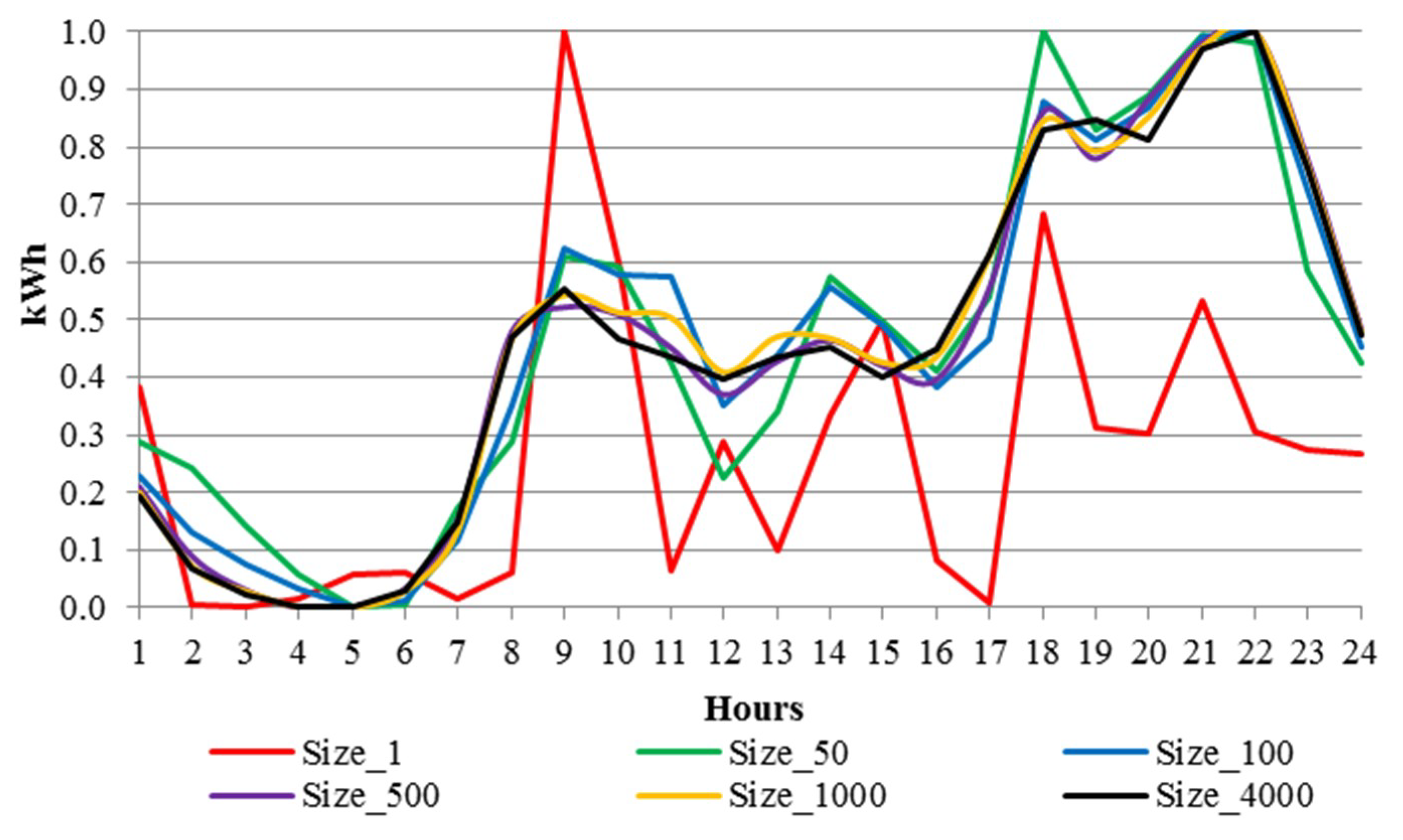
2. Smart Meter Data Used

2.1. The CER Data Set

This research is conducted based on the Irish Commission for Energy Regulation (CER) data set. The CER initiated a Smart Metering Project in 2007 with the purpose of undertaking trials to assess the performance of Smart Meters and their impact on consumer behavior. It contains measurements of electricity consumption gathered from 4182 households between July 2009 and December 2010 (75 weeks in total with 30 min data granularity). Each participating household was asked to fill out a questionnaire before and after the study. The questionnaire contained inquiries regarding the consumption behavior of the occupants, the household’s socio-economic status, properties of the dwelling and appliance stock [20].

Some characteristics of the underlying data are presented in Figure 1, where the normalized consumption observed at different aggregation levels is visualized. Aggregation reduces the variability in electricity consumption resulting in increasingly smooth load shapes when at least 100 households are considered.

Figure 1. Hourly electricity consumption for various aggregation levels.

The CER data set, to the best of our knowledge, does not account for energy that is consumed by heating and cooling systems. The heating systems of the participating households either use oil or gas as a source of energy or their consumption is measured by a separate electricity meter. The households registered in the project were reported to have no cooling system installed [20].

2.2. Features

The definition of features vector is crucial to the success of any classifier based on a machine learning algorithm. To make the high-volume time series data applicable to the classification problem, they have to be transformed into a number of representative variables. As suggested in [10,20], features can be divided in four groups: consumption features, ratios, temporal features, and statistics. This set of features especially considers the relation between the consumption on weekdays and on the weekend, parameters of seasonal and trend decomposition, estimation of the base load and some statistical features (please refer to Table 1). Altogether the attributes describe consumption characteristics (such as mean consumption at different times of the day and on different days), ratios (e.g., daytime-ratios and ratios between different days), statistical aspects (e.g., the variance, the auto-correlation and other statistical numbers) and finally different temporal aspects (such as consumption levels, peaks, important moments, temporal deviations, values of time series analysis) [10,20].

Table 1. List of 91 features used in the analysis.

Consumption	Ratios	Statistical	Temporal
c_week	r_night_day	s_variance	t_above_base
c_weekday	r_morning_noon	s_cor_wd	t_above_1kw
c_weekend	r_evening_noon	s_num_peaks	t_above_2kw
c_evening	r_mean_max	s_diff	t_above_mean
c_morning	r_min_mean	s_q1	t_daily_max
c_night	r_evening_wd_we	s_q2	t_daily_min
c_noon	r_night_wd_we	s_q3	ts_acf_mean3h
c_min	r_morning_wd_we	s_min_avg	ts_acf_mean3h_weekday
c_max	r_noon_wd_we	s_max_avg	ts_stl_varRem
c_we_max	r_afternoon_wd_we	s_var_we	b_day_diff
c_we_evening	r_min_wd_we	s_var_wd	b_day_weak
c_wd_evening	r_max_wd_we	s_cor_wd_we	wide_peaks
c_we_night	r_var_wd_we	s_cor_we	width_peaks
c_wd_night	r_we_night_day	n_d_diff	sm_variety
c_we_morning	r_wd_night_day	number_zeros	bg_variety
c_wd_morning	r_we_morning_noon		time_above_base2
c_we_noon	r_wd_morning_noon		percent_above_base
c_wd_noon	r_we_evening_noon		value_above_base
c_we_afternoon	r_wd_evening_noon		const_time
c_wd_afternoon	r_mean_max_no_min		value_min_guess
c_afternoon	r_evening_noon_no_min		first_above_base
c_we_min	r_morning_noon_no_min		number_big_peaks
c_wd_max	r_day_night_no_min		number_small_peaks
c_wd_min			dist_big_v
c_sm_max
c_evening_no_min
c_morning_no_min
c_night_no_min
c_noon_no_min

All attributes were created based on time series, so we did not apply any dimensionality reduction techniques e.g., Principal Component Analysis in order not to reduce interpretability of a particular variable and to prevent information loss. After the feature extraction, the values are normalized. To evaluate algorithms, we have separated the data into training and testing dataset at a 70%:30% ratio.

3. Grade Data Analysis

In the following lines, Grade Data Analysis is presented. It is an interesting technique that works on variables measured on any scale, including categorical. The method uses dissimilarity measures including concentration curves and the measure of monotonic dependence. The framework is based on grade transformation proposed by [21], and developed by [22]. The general idea is to transform any distribution of two variables into a structure that enables to capture the underlying dependencies of the so-called grade distribution. In practical applications, the grade data approach consists of analyzing the two-way table with rows/columns, which is preceded by proper recoding of variable values and providing the values of monotone dependence measures like Spearman’s ${\rho }^{*}$ and Kendall’s $\tau$.

The main component of the grade methods is Grade Correspondence Analysis (GCA), which stems from classical correspondence analysis. Importantly, Grade Data Analysis is going significantly beyond the correspondence approach, thanks to the means of grade transformation. An important feature of GCA is that it does not create a new measure but takes into account the original structure of the underlying phenomenon. GCA performs multiple ordering iterations on both the columns and the rows of the table, in such a way that neighboring rows are more similar than those further apart, and at the same time, neighboring columns are more similar than those that are further apart. Once the optimal structure is found, it is possible to combine neighboring rows and neighboring columns, and therefore, to build the clusters representing similar distributions. The Spearman ${\rho }^{*}$ was originally proposed for continuous distributions, however it may be defined also as Pearson’s correlation applied to the distribution after the grade transformation. Importantly, the grade distribution is applicable for discrete distribution too, and it is possible to calculate Spearman ${\rho }^{*}$ for the probability table P with m rows and k columns, where p_is is the probability of i-th row in s-th column:

$${\rho }^{*}\left(P\right)=3{\displaystyle \sum }_{i=1}^m{\displaystyle \sum }_{s=0}^k\left(p_{is}\left(2S_{row\left(i\right)}-1\right)\left(2S_{col\left(s\right)}-1\right)\right),$$

(1)

where

$$S_{row\left(i\right)}=\left({\displaystyle \sum }_{j=1}^{i-1}{p}_{j+}\right)+\frac{1}{2}{p}_{i+}, S_{col\left(s\right)}=\left({\displaystyle \sum }_{t=1}^{s-1}{p}_{+t}\right)+\frac{1}{2}{p}_{+s}$$

(2)

and $p_{j+}$ and ${\mathrm{p}}_{+\mathrm{t}}$ are marginal sums defined as: $p_{j+}={{\displaystyle \sum }}_{s=1}^k{p}_{js}, p_{+t}={{\displaystyle \sum }}_{t=1}^m{p}_{ts}$.

GCA is supposed to maximize ${\rho }^{*}$ by ordering the columns and the rows taking into account their grade regression value, which represents the gravity center for each column or each row. The grade regression for the rows is defined as:

$$reg{r}_{row\left(i\right)}=\frac{{{\displaystyle \sum }}_{s=1}^k{p}_{is}{S}_{col\left(s\right)}}{p_{i+}}$$

(3)

and, similarly, for the columns:

$$reg{r}_{col\left(s\right)}=\frac{{{\displaystyle \sum }}_{i=1}^m{p}_{is}{S}_{row\left(i\right)}}{p_{+s}}.$$

(4)

The idea behind the algorithm is to measure the grade regression for columns and to sort the columns by its values, which results in an increase of the regression for columns. At the same time, the regression for rows changes as well. Similarly, if the regression for rows is sorted then regression for columns changes. As evidenced in [23], each sorting iteration with respect to grade regression values, in fact, increases the value of Spearman ${\rho }^{*}$. The number of possible combinations with rows and columns permutations is finite and it is equal to $\mathrm{k}!\mathrm{m}!$. With the increasing value of Spearman ${\rho }^{*}$, the last sorting iteration produces the largest ${\rho }^{*}$, called local maximum of Spearman ${\rho }^{*}$.

In consecutive steps, GCA randomly permutes rows and columns and reorders them so local maximum can be achieved. In practical application, when the data volume and dimension is huge, the search over the all possible combinations of rows and columns is a computationally demanding and long-lasting process. Therefore, in order to find a global maximum of ${\rho }^{*}$, Monte Carlo simulations are used. To achieve it, the algorithm is iteratively searching for such a representation where ${\rho }^{*}$ reaches local maximum, starting from randomly ordered rows and columns. From the whole set of local maxima, the highest value of ${\rho }^{*}$ is chosen and it is assumed to be close to the global maximum, which usually happens after 100 iterations of the algorithm. Importantly, the calculation of grade regression requires non-zero sum for each and every row and column in a table, so this requirement is applicable also to the GCA. A more detailed description on grade transformation mechanics can be found in [22,24].

As far as grade cluster analysis (GCCA) is concerned, its framework is based on optimal permutations provided by the GCA. The following assumptions are associated with the cluster analysis: the number of clusters is provided, and the rows and columns of the data table (variables, say $\mathrm{X}$ and $\mathrm{Y}$) are optimally aggregated. The respective, aggregated probabilities in the table for cluster analysis, are derived from the sums of component probabilities which are found in initial, optimally ordered table, and number of rows in the aggregated table equals the specified number of clusters. The optimal clustering is supposed to be achieved when ${\rho }^{*}$($\mathrm{X}$, $\mathrm{Y}$) is maximal in the set of aggregated rows and/or columns, which are adjacent in optimal permutations. The rows and the columns may be combined either separately–by maximizing ${\rho }^{*}$ for aggregated $\mathrm{X}$ and non-aggregated $\mathrm{Y}$, or for non-aggregated $\mathrm{X}$ and aggregated $\mathrm{Y}$, or simultaneously. Details of the maximization procedure can be found in [23].

Finally, the grade analysis is highly supported by visualizations using over-representation maps. The maps are acting as a very convenient tool for plotting both source and transformed data structures where the idea is to show the various structures in the data with respect to the average values. Every cell in the data table is covered by the respective rectangle in $\left[0,1]\times [0,1\right]$ space and it is visualized using shades of grey, which corresponds to the level of the randomized grade density. The scale of grade density is divided into several intervals and respective colors represent particular intervals, with black corresponding to the highest values and white corresponding to the lowest. With the grade density used to measure the deviation from independence of variables $\mathrm{X}$ and $\mathrm{Y}$, the dark colors indicate overrepresentation while the white ones show underrepresentation.

4. GCA Clustering Experiments

The starting point for the experiments was to prepare the initial matrix with normalized features $\left({\mathrm{x}}_{\mathrm{i}}-\min \left(\mathrm{x}\right)\right)/\left(\max \left(\mathrm{x}\right)-\min \left(\mathrm{x}\right)\right)$ in the columns and the rows representing each of the households. The structure of the dataset is presented in Table 2.

Table 2. The sample matrix with the features extracted for each of the households.

Household	Feature_1	Feature_2	…	Feature_91
1	0.23	0.57	…	0.85
2	0.64	0.77	…	0.27
…	…	…	…	…
4182	0.51	0.73	…	0.63

The data structure presented in Table 2 has been analyzed using GradeStat software [25], which is the tool that was developed in the Institute of Computer Science Polish Academy of Science.

The next step was to compute over-representation ratios for each field (cell) of the table with households and the attributes describing them. For a given $m\times k$ data matrix with non-negative values, a visualization using over-representation map is possible, in the same way as a contingency table. However, instead of frequency $n_{ij}$ the value of $j$-th feature for $i$-th household is used. Subsequently, it is compared in a contingency table with the corresponding neutral or fair representation of $n_{i•}\times n_{•j}/\sum \sum n_{ij}$ where $n_{i•}={{\displaystyle \sum }}_j{n}_{ij}$, $n_{•j}={{\displaystyle \sum }}_i{n}_{ij}$. The ratio of the expression is called the over-representation. An over-representation surface over a unit square is then divided into $m\times k$ cells situated in $m$ rows and $k$ columns, and the area of cells placed in row $i$ and column $j$ is assumed to be equal to fair representation of normalized $n_{ij}$. Based on the over-representation ratios, the over-representation map for the initial raw data can be constructed. The color intensity of each cell in the map is the result of the comparison between two values: (1) the real value of the measure connected to the underlying cell; (2) the expected value of the measure. In Figure 2 there is an initial over-representation map for the analyzed data presented. The colors of the cells in the map are grouped into three classes representing different properties:

Figure 2. The initial over-representation map.

• gray–the feature for the element (household) is neutral (ranging between the 0.99–1.01) which means that the real value of the feature is equal to its expected value;
• black or dark gray–the feature for the element (household) is over-represented (between 1.01 and 1.5 for weak over-representation and more than 1.5 for strong) which means that the real value of the feature is greater than the expected one;
• light gray or white–the feature for the element (household) is under-represented (between 0.66 and 0.99 for weak under-representation and less than 0.66 for strong under-representation), which means that the real value of feature is less than the expected one.

Besides the differences in color’s scales on the map—its rows and columns could be of different sizes. A row’s height depends on the evaluation of the element (household) in comparison to the entire population, so the households with higher evaluation are represented by higher rows. A column’s width depends on the evaluation of the element (feature) in comparison to the evaluation of all the features from the set, so the features with higher evaluation are represented by wider columns.

In order to reveal the structural trends in data, the following step was to apply the grade analysis to measure the dissimilarity between analyzed data distributions—households and feature dimensions. The grade analysis was conducted based on Spearman’s ${\rho }^{*}$, used as the total diversity index. The value of ${\rho }^{*}$ strongly depends on the mutual order of the rows and the columns and therefore, to calculate ${\rho }^{*}$, the concentration indexes of differentiation between the distributions were used. The basic GCA procedure is executed through permuting the rows and columns of a table in order to maximize the value of ${\rho }^{*}$. After each sorting, the ${\rho }^{*}$ value increases and the map becomes more similar to the ideal one. As presented on the maps, the darkest fields are placed in the upper-left and the lower-right corners while the rest of the fields are assigned according to the following property: the farther from the diagonal towards the two other map corners (the lower-left and the upper-right ones) the lighter gray (or white) color the fields have.

The result of the GCA procedure is presented in Figure 3. The rows represent households and the columns represent the features describing the households. The resulting order presents the structure of underlying trends in data. The analysis of the map reveals that two groups of the features can be distinguished: the features which non-differentiate the population of households (the middle columns of the map) and those which differentiate the households (the most-left and the most-right columns).

Figure 3. The final over-representation map with four clusters.

Four vertical clusters were marked in Figure 3 (C1, C2, C3 and C4) and these show typical behavior of the households in terms of the electricity usage characterized by the respective number of features (in brackets).

Finally, the aggregation of some rows representing unique households was performed. The optimal number of four clusters was obtained when the changes of the subsequent ${\rho }^{*}$ values appeared to be irrelevant as referenced in [22]. In Figure 4, the chart with the ${\rho }^{*}$ values as a function of the number of clusters is presented. The points on the $OX$ axis correspond to the cluster numbers. The $OY$ axis is denoted by the values of ${\rho }^{*}$.

Figure 4. The ${\rho }^{*}$ values for different number of clusters.

The proposed GCA method applied for the clustering enables identification of the features describing different aspects of the consumption behaviors. The clusters are further utilized to select representative features within each cluster to be used for revealing selected households’ characteristics.

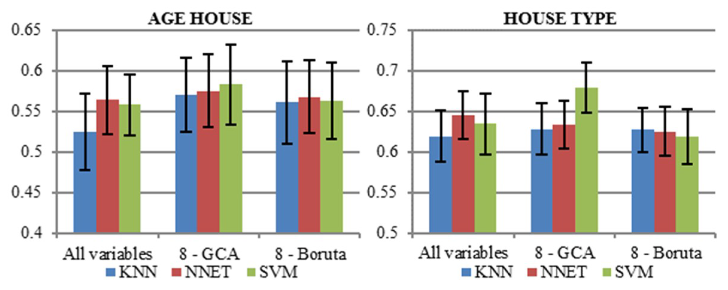
5. Classification of Selected Household Characteristics

5.1. Problem Statement

In the following lines we present and assess a classification system that applies supervised machine learning algorithms to automatically reveal specific patterns or characteristics of the households, having their aggregated electricity consumption as an input. The patterns/characteristics are related to the socio-economic status of a particular household and its dwelling. In particular, the following properties are explored:

• Family type;
• Number of bedrooms;
• Number of appliances;
• Employment;
• Floor area;
• House type;
• House age;
• Householder age.

Along with the detailed smart metering data, the data set provides information on the characteristics of each household collected through the questionnaires. Such information delivers true output to classification to validate the proposed models. Table 3 presents eight questionnaire questions that were used as the target features for classification (true outcome).

Table 3. Questionnaire questions and their corresponding category labels.

Category	Person’s Age	Number of Appliances
	What Age Were You on Your Last Birthday?	Approximately How Many Appliances Are in Your Home?
1	18–35	≤8 appliances
2	36–65	between 9 and 11
3	65+	>11 appliances
Category	Number of Bedrooms	Floor Area
	How many bedrooms are in your home?	Approximately what is the area of your home?
1	≤2 bedrooms	Not available
2	3 bedrooms	<100 m2
3	4 bedrooms	between 100 m2 and 200 m2
4	≥5 bedrooms	>200 m2
Category	Employment	Family type
	What is the employment status of the chief income earner in your household?	What best describes the people you live with?
1	An employee, Self-employed (with employees), Self-employed (with no employees)	I live alone
2	Unemployed (actively seeking work), Unemployed (not actively seeking work), Retired, Carer: Looking after relative family	All people in my home are over 15 years of age, both adults and children under 15 years of age live in my home
Category	House Age	House Type
	Approximately how old is your home?	Which best describes your home?
1	≤30 years	Semi-detached house, Terraced house
2	>30 years	Apartment, Detached house, Bungalow

For classification of the households’ properties, three experimental feature setups were considered:

• All the variables (91) were used in the algorithms;
• Eight variables based on GCA and selected as representatives of each cluster having the highest AUC measure (please refer to Appendix A, Table A1);
• Eight variables based on Boruta package which is the feature selection algorithm for finding relevant variables [26].

5.2. Accuracy Measures

For the purpose of model evaluation, four performance measures were used, i.e., classification accuracy, sensitivity, specificity and area under the ROC curve (AUC) [27]. For the binary classification problem, i.e., having positive class and negative class, four possible outcomes exist, as shown in Table 4.

Table 4. Confusion matrix for binary classification.

		Predicted Value
		Positive (P)	Negative (N)
Real Value	Positive (P)	True positive (TP)	False negative (FN)
	Negative (N)	False positive (FP)	True negative (TN)

Based on Table 4, the accuracy (AC) measure can be computed, which is the proportion of the total number of predictions that were correct:

$$AC=\frac{TP+TN}{TP+FP+TN+FN}.$$

(5)

AUC estimation requires two indicators defined as: true positive rate $Tpr=\frac{TP}{TP+FN}$, and false positive rate $Fpr=\frac{FP}{FP+TN}=1-Tnr$. These measures can be calculated for different decision threshold values. An increase of the threshold from 0 to 1 will yield a series of points $\left(Fpr, Tpr\right)$ constructing the curve with $Tpr$ and $Fpr$ on the horizontal and vertical axes, respectively. In a general form, the value of AUC is given by $AUC={{\displaystyle \int }}_0^{1}ROC\left(u\right)du.$

From another point of view, AUC can be understood as $P\left(X_p>X_n\right)$ where $X_p$ and $X_n$ denote the markers for positive and negative cases, which can be interpreted as the probability that in a randomly drawn pair of positive and negative cases, the classifier probability is higher for the positive one.

5.3. Classification Algorithms

Building predictive models involves complex algorithms, therefore R-CRAN was used as the computing environment. In this research, all the numerical calculations were performed on a personal computer equipped with an Intel Core i5-2430M 2.4 GHz processor (2 CPU × 2 cores), 8 GB RAM and the Ubuntu 16.04 LTS operating system. To achieve predictive models having good generalization abilities, special learning process incorporating AUC measure was performed. Because of this, the following maximized function assures the best parameters of each algorithm:

$$f\left(AU{C}_T,AU{C}_V\right)=-\frac{1}{2}\left|AU{C}_T-AU{C}_V\right|+\frac{1}{2}AU{C}_V,$$

(6)

where $AU{C}_T$ stands for the training accuracy, and $AU{C}_V$ stands for the validation accuracy.

5.3.1. Artificial Neural Networks

Artificial neural networks (ANN) are mathematical objects in the form of equations or systems of equations, usually nonlinear, for analysis and data processing. The purpose of neural networks is to convert input data into output data with a specific characteristic or to modify such systems of equations to read useful information from their structure and parameters. On a statistical basis, selected types of neural networks can be interpreted in general non-linear regression categories [28].

In studies related to forecasting in power engineering, multilayer, one-way artificial neural networks with no feedback are most commonly used. Multilayer Perceptron networks (MLP) are one of the most popular types of supervised neural networks. For example, the MLP network (3, 4, 1) means a neural network with three inputs, four neurons in the hidden layer and one neuron in the output layer. In general, the three-layer MLP neural network ($\mathrm{P}, \mathrm{M}, \mathrm{K}$) is described by the expression:

$$f\left(x_i,w\right)=h_2\left({\mathit{W}}_2\left[h_1\left({\mathit{W}}_1{x}_i+{\mathit{b}}_1\right)\right]+{\mathit{b}}_2\right),$$

(7)

where $x_i={\left(x_1,\dots ,x_p\right)}^T$ represents the input data, ${\mathit{W}}_1$ is the matrix of the first layer weights with dimensions $M\times P$, ${\mathit{W}}_2$ is the matrix of the second layer weights with dimensions $K\times M$, $h_i\left(\mathit{u}\right)$ and ${\mathit{b}}_i$ are nonlinearities (functions of neuron activation e.g., logistic function) and constant values in subsequent layers respectively [28].

The goal of supervised learning of the neural network is to search for such network parameters that minimize the error between the desired values $L_i$ and received at the output of the network $P_i$. The most frequently minimized error function is the sum of the squares of differences between the actual value of the explained variable and its theoretical value determined by the model, with the values of the synaptic weight vector set:

$$E\left(w\right)=\frac{1}{2}{\displaystyle \sum }_{k=1}^K{e}^{\left(k\right)}=\frac{1}{2}{\displaystyle \sum }_{k=1}^K\left({\displaystyle \sum }_{i=1}^n{\left(P_i^{\left(k\right)}-L_i^{\left(k\right)}\right)}^2\right),$$

(8)

where $n$ is the number of the training sample, $P_i^{\left(k\right)}$ and $L_i^{\left(k\right)}$ are predicted and reference value and $K$ is the number of training epochs of the neural network [28].

The neural network learning process involves the iterative modification of the values of the synaptic weight vector $\mathit{w}$ (all weights are set in one vector), in iteration $k+1$:

$${\mathit{w}}_{k+1}={\mathit{w}}_k+{\eta }_k{\mathit{p}}_k,$$

(9)

where ${\mathit{p}}_k$ is the direction of the minimization of the function $E\left(w\right)$ and $\eta$ is the magnitude of the learning error. The most popular optimization methods are undoubtedly gradient methods, which are based on the knowledge of the function gradient:

$${\mathit{p}}_k=-{\left[\mathit{H}\left({\mathit{w}}_k\right)\right]}^{-1}\mathit{g}\left({\mathit{w}}_k\right),$$

(10)

where $\mathit{g}$ and $\mathit{H}$ denote the gradient and the hesian of the last known solution ${\mathit{w}}_k$, respectively [28].

In the practical implementations of the algorithm, the exact determination of hesian $\mathit{H}\left({\mathit{w}}_k\right)$ is abandoned, and its approximation $\mathit{G}\left({\mathit{w}}_k\right)$ is used instead. One of the most popular methods of learning neural networks is the algorithm of variable metrics. In this method, the hesian (or its reversal) in each step is modified from the previous step by some correction. If by $c_k$ and $r_k$ the increments of the vector $\mathrm{w}$ and the gradient $\mathit{g}$ in two successive iterative steps are marked, ${\mathit{c}}_k={\mathit{w}}_k-{\mathit{w}}_{k-1}$, ${\mathit{r}}_k={\mathit{g}}_k-{\mathit{g}}_{k-1}$, and by ${\mathit{V}}_k$ the inverse matrix of the approximate hessian ${\mathit{V}}_k={\left[\mathit{G}\left({\mathit{w}}_k\right)\right]}^{-1}$, ${\mathit{V}}_{k-1}={\left[\mathit{G}\left({\mathit{w}}_{k-1}\right)\right]}^{-1}$, according to the most effective formula of Broyden-Fletcher-Goldfarb-Shanno (BFGS), the process of updating the value of the ${\mathit{V}}_k$ matrix is described by the recursive relationship:

$${\mathit{V}}_k={\mathit{V}}_{k-1}+\left(1+\frac{{\mathit{r}}_k^T{\mathit{V}}_{k-1}{\mathit{r}}_k}{{\mathit{c}}_k^T{\mathit{r}}_k}\right)\frac{{\mathit{c}}_k{\mathit{c}}_k^T}{{\mathit{c}}_k^T{\mathit{r}}_k}-\frac{{\mathit{c}}_k{\mathit{r}}_k^T{\mathit{V}}_{k-1}+{\mathit{V}}_{k-1}{\mathit{r}}_k{\mathit{c}}_k^T}{{\mathit{c}}_k^T{\mathit{r}}_k}.$$

(11)

As a starting value ${\mathit{V}}_0=1$ is usually assumed, and the first iteration is carried out in accordance with the algorithm of the largest slope [28].

Artificial neural networks are often used to estimate or approximate functions that can depend on a large number of inputs. In contrast to the other machine learning algorithms considered in these experiments, the ANN required the input data to be specially prepared. The vector of continuous variables was standardized, whereas the binary variables were converted such that 0 s were transformed into values of −1 [3,5,29].

To train the neural networks, we used the BFGS algorithm implemented in the nnet library. The network had an input layer with 91 neurons and a hidden layer with 1, 2, 3, …, 15 neurons. A logistic function was used to activate all of the neurons in the network. To achieve robust estimation of the neural networks error, 10 different neural networks were learned with different initial weights vector. Final estimation of the error was computed as the average value over 10 neural networks [3,5,29].

In each experiment, 15 neural networks were learned with various parameters (the number of neurons in the hidden layer). To avoid overfitting, after each learning iteration had finished (with a maximum of 50 iterations), the models were checked using the measure defined in (6). Finally, out of the 15 learned networks, that with the highest value was chosen as the best for prediction [3,5,29].

5.3.2. K-Nearest Neighbors Classification

The $k$-nearest neighbors (KNN) regression [30] is a non-parametric method, which means that no assumptions are made regarding the model that generates the data. Its main advantage is the simplicity of the design and low computational complexity. The prediction of the value of the explained variable $L_i$ on the basis of the vector of explanatory variables ${\mathit{x}}_i$ is determined as:

$$P_i=\frac{{{\displaystyle \sum }}_{k=1}^K{L}_k I\left({\mathit{x}}_i,{\mathit{x}}_k\right)}{K},$$

(12)

where:

$$I\left({\mathit{x}}_i,{\mathit{x}}_k\right)=\{\begin{array}{c}1, if x_k \mathrm{is} \mathrm{one} \mathrm{of} the k \mathrm{nearest} \mathrm{neighbors} {\mathit{x}}_i\\ 0, \mathrm{otherwise}\end{array},$$

(13)

whereas ${\mathit{x}}_k$ is one of the $k$-nearest neighbors ${\mathit{x}}_i$, in the case where the distance $d\left({\mathit{x}}_i,{\mathit{x}}_k\right)$ belongs to $k$, the smallest distance between the observations from the set $X$ and ${\mathit{x}}_k$. The most commonly used distance is the Euclid distance [3,5,29,30].

To improve the algorithm, we normalized the explanatory variables (standardization for quantitative variables and replacement of 0 by −1 for binary variables). The normalization ensures that all dimensions for which the Euclidean distance is calculated have the same importance. Otherwise, a single dimension could dominate the other dimensions [3,5,29].

The algorithm was trained with knn implemented in the caret library. Different values of $k$ were investigated in the experiments: {5, 10, 15, 20, 25, 30, 35, 40, 45, 50, 55, 60, 65, 70, 75, 80, 85, 90, 95, 100, 110, 120, 130, 140, 150, 160, 170, 180, 190, 200, 250, 300}. The optimal value, and thus the final form of the model, was determined as that giving the maximum value according to (6) [3,5,29].

5.3.3. Support Vector Classification

Support Vector learning is based on simple ideas which originated in statistical learning theory [31]. The simplicity comes from the fact that Support Vector Machines (SVMs) apply a simple linear method to the data but in a high-dimensional feature space non-linearly related to the input space. Moreover, even though we can think of SVMs as a linear algorithm in a high-dimensional space, in practice, it does not involve any computations in that high-dimensional space [28].

SVMs use an implicit mapping $\mathsf{\Phi }$ of the input data into a high-dimensional feature space defined by a kernel function, i.e., a function returning the inner product $⟨\mathsf{\Phi }\left({\mathit{x}}_i\right),\mathsf{\Phi }\left({\mathit{x}}_i^{\prime }\right)⟩$ between the images of two data points ${\mathit{x}}_i$, ${\mathit{x}}_i^{\prime }$ in the feature space. The learning then takes place in the feature space, and the data points only appear inside dot products with other points [32]. More precisely, if a projection $\mathsf{\Phi }:\mathit{X}\to \mathit{H}$ is used, the dot product ⟨$\mathsf{\Phi }\left({\mathit{x}}_i\right),\mathsf{\Phi }\left({\mathit{x}}_i^{\prime }\right)$⟩ can be represented by a kernel function $k$ which is computationally simpler than explicitly projecting ${\mathit{x}}_i$ and ${\mathit{x}}_i^{\prime }$ into the feature space $\mathit{H}$ [28].

Training an SVM involves solving a quadratic optimization problem. Using a standard quadratic problem solver for training an SVM would involve solving a big QP problem even for a moderately sized data set, including the computation of an $n\times n$ matrix in memory ($n$ number of training points). In general, predictions correspond to the decision function:

$$P_i=\mathrm{sign}(⟨\mathit{w},\mathsf{\Phi }\left({\mathit{x}}_i\right)⟩),$$

(14)

where solution $\mathit{w}$ has an expansion $\mathit{w}={\alpha }_i{\displaystyle \sum }_i\mathsf{\Phi }\left({\mathit{x}}_i\right)$ in terms of a subset of training patterns that lie on the margin [25].

In the case of the L2-norm soft margin classification, the primal optimization problem takes the form:

$$\mathrm{minimize} \left(t,\mathit{w}\right)=\frac{1}{2}{||\mathit{w}||}^2+\frac{C}{n}{\displaystyle \sum }_{i=1}^n\left({\xi }_i\right),$$

(15)

$$\begin{array}{c}subject to L_i(⟨\Phi \left({\mathit{x}}_i\right),\mathit{w}⟩+b)\le 1-{\xi }_i^{*}\\ {\xi }_i\ge 0 \left(i=1,\dots ,n\right)\end{array},$$

(16)

where $n$ is the number of training patterns, and $L_i\mp 1$, $C$ is the cost parameter that controls the penalty paid by the SVM for misclassifying a training point and thus the complexity of the prediction function. A high cost value $C$ will force the SVM to create a complex enough prediction function to misclassify as few training points as possible, while a lower cost parameter will lead to a simpler prediction function.

To construct the support vector machine model, $C$-SVR from the kernlab library with sequential minimal optimization (SMO) was used to solve the quadratic programming problem. A linear, polynomial (of degree 1, 2 and 3) and radial ($\gamma$ from 0.1 to 1 by 0.2) kernel function were used, and $\epsilon$ (which defines the margin width for which the error function is zero) was arbitrarily taken from the following set {0.1, 0.3, 0.5, 0.7, 0.9}. The regularized parameter $C$ that controls overfitting was arbitrarily set to one of the following values {0, 0.2, 0.4, 0.6, 0.8, 1}. Finally, as in all previous cases, the model that maximized the function (6) was chosen [29].

5.4. Classification Results

This section refers to application of classification algorithms mentioned in Section 5.3. For the sake of clarity and synthesis, the results are visualized and provided for the testing dataset only. However, in the appendix section the detailed results for each algorithm and for three feature sets are presented (Appendix B).

Additionally, in Appendix C the final set of independent variables used in classification models and for each dependent variable was provided.

As far as summary results are concerned, Figure 5 shows the accuracy achieved by the algorithms–KNN, NNET and SVM with break down into three feature selection techniques—All variables, 8 GCA, 8 Boruta. From the left to the right are the results for family type, number of bedrooms, employment type, floor area, house type, number of appliances, householder age and house age. The whiskers represent standard deviations.

Figure 5. Classification accuracy.

It can be observed that the methods achieve approx. 90% accuracy for classification of appliances and age of the house, regardless of the classification algorithm. Family type is classified with nearly 75% accuracy. On the other hand, the most difficult characteristic to be discovered by algorithms is number of bedrooms, with the accuracy reaching only 50%.

In terms of different approaches for features selection, it was observed that proposed GCA algorithm (8-GCA), used for clustering variables and selecting only two representatives of the clusters, worked well and can be considered as a technique for feature selection. Broader set of all variables was relevant for classification of floor area only.

The next figure, Figure 6, illustrates the AUC values for the classifiers. The range of AUC values between analyzed households’ characteristics vary from 0.52 (for age of the house and using KNN) to 0.82 (for family type, regardless classification algorithm). Overall, all variables are necessary to result in high AUC only for classification of main inhabitant’s age and floor area. For other characteristics, using 8 variables, either GCA or Boruta, resulted in equally good classification measured by AUC.

Figure 6. Area Under Receiver Operating Curve (AUC) values.

In general, the results indicate that the choice of a classification model should depend on the specific target application. In the experiment it was observed that SVM and NNET stand out as the classifiers that allow to achieve the best performance. However, the results may vary taking into account variable selection mechanism.

6. Conclusions

The approach presented in this paper shows that classification of households’ socio-demographic and dwelling characteristics based on the electricity consumption is feasible and gives the opportunity to derive additional knowledge about the customers.

In practice, such knowledge can motivate electricity providers to offer new and more customer-oriented energy services. With growing liberalization of the energy market, premium and non-standard services may represent a competitive advantage to both existing customers and new ones.

The experimental results reported in Section 5 show that selected classification algorithms can reveal household characteristics from electricity consumption data with fair accuracy. In general, the choice of a particular classifier should depend on the specific target application. In the experiment, it was observed that SVM and NNET delivered equally good performance, however the results varied depending on the variable selection procedure. For six out of eight household characteristics, using only eight variables, either GCA or Boruta resulted in a satisfactory level of accuracy.

The GCA proposed in this article allowed for quickly grasping general trends in data, and then to cluster the attributes, taking into account historical electricity usage. It is worth underlining that the method was competitive with the Boruta algorithm, having its roots in random forest algorithms. The results obtained by grade analysis might be the basis not only for feature selection but also for the customers’ segmentation.

Since the results are promising, we aim, as an extension to this research, to focus on a broader set of variables including external factors like weather information (including humidity, temperature, sunrises and sunsets) as well as holidays and observances (including school holidays). The other direction for future research may involve application of selected segmentation algorithms to extract homogeneous groups of customers and to look for specific socio-demographic characteristics within the clusters.

References

1. Chicco, G. Overview and performance assessment of the clustering methods for electrical load pattern grouping. Energy 2012, 421, 68–80. [Google Scholar] [CrossRef]
2. Chicco, G.; Napoli, R.; Piglione, F.; Postolache, P.; Scutariu, M.; Toader, C. Load pattern-based classification of electricity customers. IEEE Trans. Power Syst. 2004, 192, 1232–1239. [Google Scholar] [CrossRef]
3. Gajowniczek, K.; Ząbkowski, T. Short term electricity forecasting based on user behavior using individual smart meter data. Intell. Fuzzy Syst. 2015, 30, 223–234. [Google Scholar] [CrossRef]
4. Haben, S.; Singleton, C.; Grindrod, P. Analysis and clustering of residential customers energy behavioral demand using smart meter data. IEEE Trans. Smart Grid 2016, 7, 136–144. [Google Scholar] [CrossRef]
5. Gajowniczek, K.; Ząbkowski, T. Electricity forecasting on the individual household level enhanced based on activity patterns. PLoS ONE 2017, 12, e0174098. [Google Scholar] [CrossRef] [PubMed]
6. Sial, A.; Singh, A.; Mahanti, A.; Gong, M. Heuristics-Based Detection of Abnormal Energy Consumption. In International Conference on Smart Grid Inspired Future Technologies; Chong, P., Seet, B.C., Chai, M., Eds.; Springer: Cham, Switzerland, 2018; pp. 21–31. [Google Scholar]
7. Batra, N.; Singh, A.; Whitehouse, K. Creating a Detailed Energy Breakdown from just the Monthly Electricity Bill. In Proceedings of the 3rd International NILM Workshop, San Francisco, CA, USA, 14–15 May 2016. [Google Scholar]
8. Rashid, H.; Arjunan, P.; Singh, P.; Singh, A. Collect, compare, and score: A generic data-driven anomaly detection method for buildings. In Proceedings of the Seventh International Conference on Future Energy Systems Poster Sessions, Waterloo, ON, Canada, 21–24 June 2016. [Google Scholar]
9. Beckel, C.; Sadamori, L.; Santini, S. Automatic socio-economic classification of households using electricity consumption data. In Proceedings of the Fourth International Conference on Future Energy Systems, Waterloo, ON, Canada, 15 January 2013. [Google Scholar]
10. Hopf, K.; Sodenkamp, M.; Kozlovkiy, I.; Staake, T. Feature extraction and filtering for household classification based on smart electricity meter data. Comput. Sci. Res. Dev. 2016, 31, 141–148. [Google Scholar] [CrossRef]
11. Poortinga, W.; Steg, L.; Vlek, C.; Wiersma, G. Household preferences for energy-saving measures: A conjoint analysis. J. Econ. Psychol. 2003, 24, 49–64. [Google Scholar] [CrossRef]
12. Vassileva, I.; Campillo, J. Increasing energy efficiency in low-income households through targeting awareness and behavioral change. Renew. Energy 2014, 67, 59–63. [Google Scholar] [CrossRef]
13. Ehrhardt-Martinez, K. Changing habits, lifestyles and choices: The behaviours that drive feedback-induced energy savings. In Proceedings of the 2011 ECEEE Summer Study on Energy Efficiency in Buildings, Toulon, France, 1–6 June 2011. [Google Scholar]
14. Chicco, G.; Napoli, R.; Postolache, P.; Scutariu, M.; Toader, C. Customer characterization options for improving the tariff offer. IEEE Trans. Power Syst. 2003, 18, 381–387. [Google Scholar] [CrossRef]
15. Carroll, J.; Lyons, S.; Denny, E. Reducing household electricity demand through smart metering: The role of improved information about energy saving. Energy Econ. 2014, 45, 234–243. [Google Scholar] [CrossRef]
16. Anda, M.; Temmen, J. Smart metering for residential energy efficiency: The use of community based social marketing for behavioural change and smart grid introduction. Renew. Energy 2014, 67, 119–127. [Google Scholar] [CrossRef]
17. Hart, G.W. Nonintrusive Appliance Load Monitoring; IEEE: New York, NY, USA, 1992. [Google Scholar]
18. Zeifman, M.; Roth, K. Nonintrusive appliance load monitoring: Review and outlook. IEEE Trans. Consum. Electron. 2011, 57, 76–84. [Google Scholar] [CrossRef]
19. Zoha, A.; Gluhak, A.; Imran, M.A.; Rajasegarar, S. Non-intrusive load monitoring approaches for disaggregated energy sensing: A survey. Sensors 2012, 12, 16838–16866. [Google Scholar] [CrossRef] [PubMed] [Green Version]
20. Beckel, C.; Sadamori, L.; Staake, T.; Santini, S. Revealing household characteristics from smart meter data. Energy 2014, 78, 397–410. [Google Scholar] [CrossRef] [Green Version]
21. Szczesny, W. On the performance of a discriminant function. J. Classif. 1991, 8, 201–215. [Google Scholar] [CrossRef]
22. Kowalczyk, T.; Pleszczynska, E.; Ruland, F. Grade Models and Methods for Data Analysis: With Applications for the Analysis of Data Populations; Springer: Berlin/Heidelberg, Germany, 2004; Volume 151. [Google Scholar]
23. Ciok, A.; Kowalczyk, T.; Pleszczyńska, E. How a new statistical infrastructure induced a new computing trend in data analysis. In International Conference on Rough Sets and Current Trends in Computing; Springer: Berlin/Heidelberg, Germany, 1998. [Google Scholar]
24. Szczesny, W. Grade correspondence analysis applied to contingency tables and questionnaire data. Intell. Data Anal. 2002, 6, 17–51. [Google Scholar]
25. Program for Grade Data Analysis. Available online: gradestat.ipipan.waw.pl (accessed on 9 June 2018).
26. Kursa, M.B.; Rudnicki, W.R. Feature selection with the Boruta package. J. Stat. Softw. 2010, 36, 1–13. [Google Scholar] [CrossRef]
27. Fawcett, T. An introduction to ROC analysis. Pattern Recognit. Lett. 2006, 27, 861–874. [Google Scholar] [CrossRef]
28. Gajowniczek, K.; Ząbkowski, T. Simulation study on clustering approaches for short-term electricity forecasting. Complex 2018, 2018, 3683969. [Google Scholar] [CrossRef]
29. Gajowniczek, K.; Ząbkowski, T. Two-Stage Electricity Demand Modeling Using Machine Learning Algorithms. Energies 2017, 10, 1547. [Google Scholar] [CrossRef]
30. Nguyen, B.; Morell, C.; De Baets, B. Large-scale distance metric learning for k-nearest neighbours regression. Neurocomputing 2016, 214, 805–814. [Google Scholar] [CrossRef]
31. Davò, F.; Vespucci, M.T.; Gelmini, A.; Grisi, P.; Ronzio, D. Forecasting Italian electricity market prices using a Neural Network and a Support Vector Regression. In Proceedings of the 2016 AEIT International Annual Conference (AEIT), Capri, Italy, 5–7 October 2016. [Google Scholar]
32. Muandet, K.; Fukumizu, K.; Sriperumbudur, B.; Schölkopf, B. Kernel mean embedding of distributions: A review and beyond. Found. Trends Mach. Learn. 2017, 10, 1–141. [Google Scholar] [CrossRef]