A Low Cost Vision-Based Road-Following System for Mobile Robots

Abstract

Navigation is necessary for autonomous mobile robots that need to track the roads in outdoor environments. These functions could be achieved by fusing data from costly sensors, such as GPS/IMU, lasers and cameras. In this paper, we propose a novel method for road detection and road following without prior knowledge, which is more suitable with small single lane roads. The proposed system consists of a road detection system and road tracking system. A color-based road detector and a texture line detector are designed separately and fused to track the target in the road detection system. The top middle area of the road detection result is regarded as the road-following target and is delivered to the road tracking system for the robot. The road tracking system maps the tracking position in camera coordinates to position in world coordinates, which is used to calculate the control commands by the traditional tracking controllers. The robustness of the system is enhanced with the development of an Unscented Kalman Filter (UKF). The UKF estimates the best road borders from the measurement and presents a smooth road transition between frame to frame, especially in situations such as occlusion or discontinuous roads. The system is tested to achieve a recognition rate of about 98.7% under regular illumination conditions and with minimal road-following error within a variety of environments under various lighting conditions.

1. Introduction

In recent years, autonomous mobile robots have been an active research field. Navigation is one of the significant problems that need to be addressed by robots, which work in outdoor environments [1]. Laser-based navigation has been rapidly improved and is leveraged by most commercial robots or driverless cars. A continuous curvature path is generated for car-like vehicle navigation by multiple clothoids composition and parametric adjustment [2]. The clothoids composition method for path generation relies heavily on detailed and highly accurate prior maps of the environments, which give the boundary geometric constraints. However, outside of small urban areas, it is very challenging to build, store, and transmit detailed maps since the spatial scales are so large. A novel mapless driving framework is proposed for addressing the problem of maintaining detailed maps of large areas, which combines sparse topological maps for global navigation with a laser-based perception system for local navigation [3]. However, the technical issue of laser-based navigation techniques is the reduction of the prior information because most of them require a precise 2D or 3D model of the environment. The lasers are comparative costly. In contrast, vision-based systems provide natural and powerful information of the environment at a high frame rate with a wide field of view. Image data captured by vision sensors contain rich information, such as luminance, color, texture, etc. Moreover, vision sensors are inexpensive compared to laser sensors. Thus, it could become a reliable complement of the laser-based navigation strategies.

The laser-based navigation method relies strongly on accurate prior maps and is very expensive. In this paper, a low-cost, vision-based road-following system is proposed for autonomous mobile robots working in outdoor environments. Our main algorithm consists of two steps, namely, road detecting and road tracking. In the road detecting system, the road is extracted by fusing the results of a color-based road detector and a texture line detector. The UKF is adopted to track the road and the extracted following target. Then, in the road-tracking system, the road-following position in world coordinate frame is calculated by the surrounding box of the target in images. The contributions of this paper can be summarized as follows:

(1)

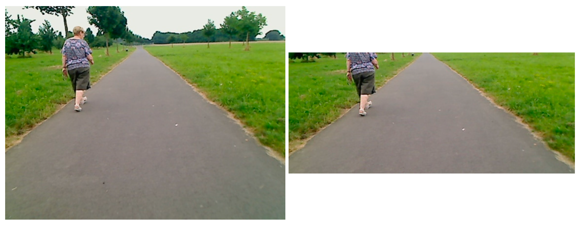
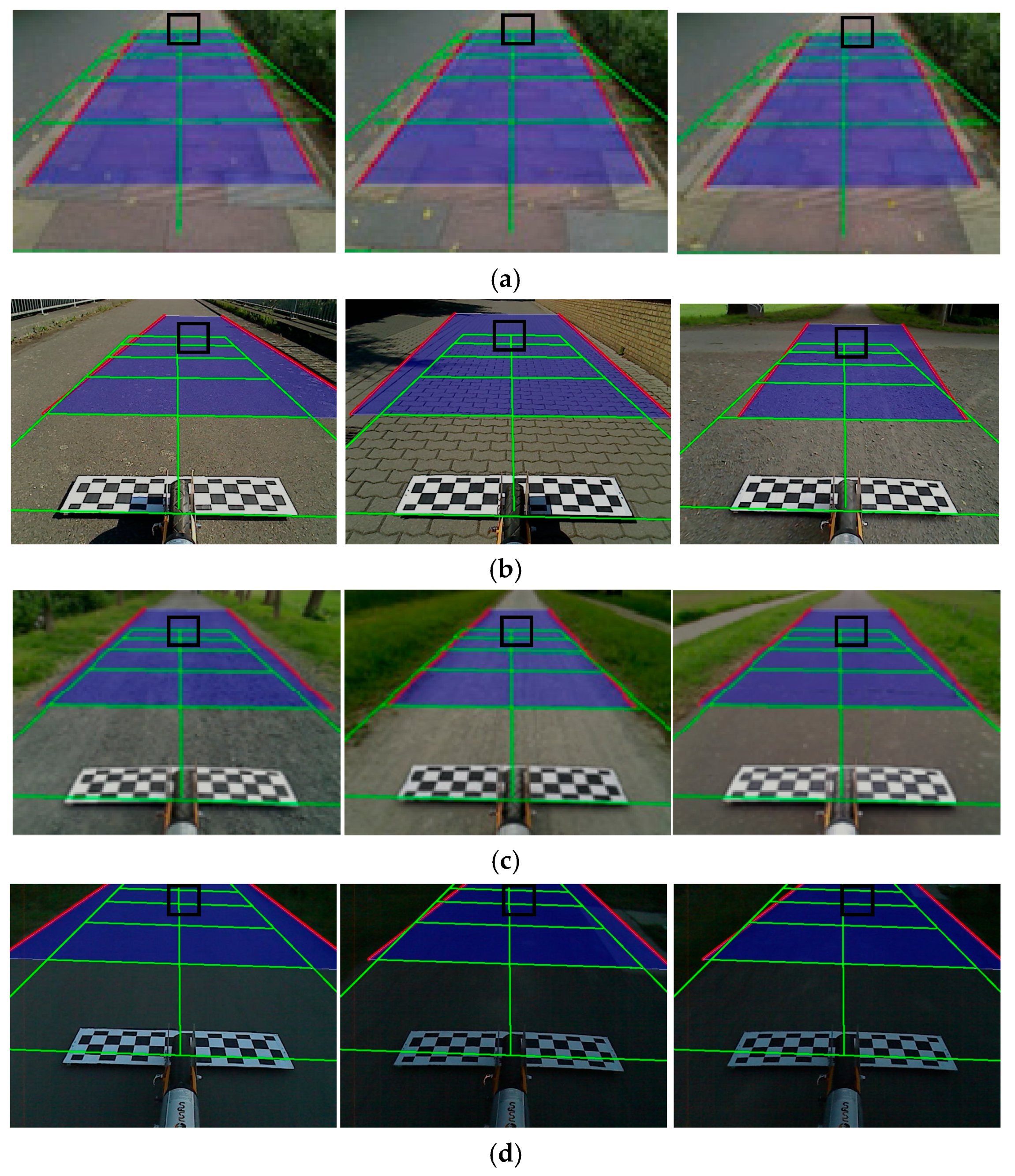
In order to have the ability to detect the road in the majority of cases, the system combines the detection of a color-based road detector and texture line detector. Benefiting from the combination of the two detectors, the proposed road-following system is more suitable with small single lane roads, such as sidewalks, bikeways, parkways, etc.

(2)

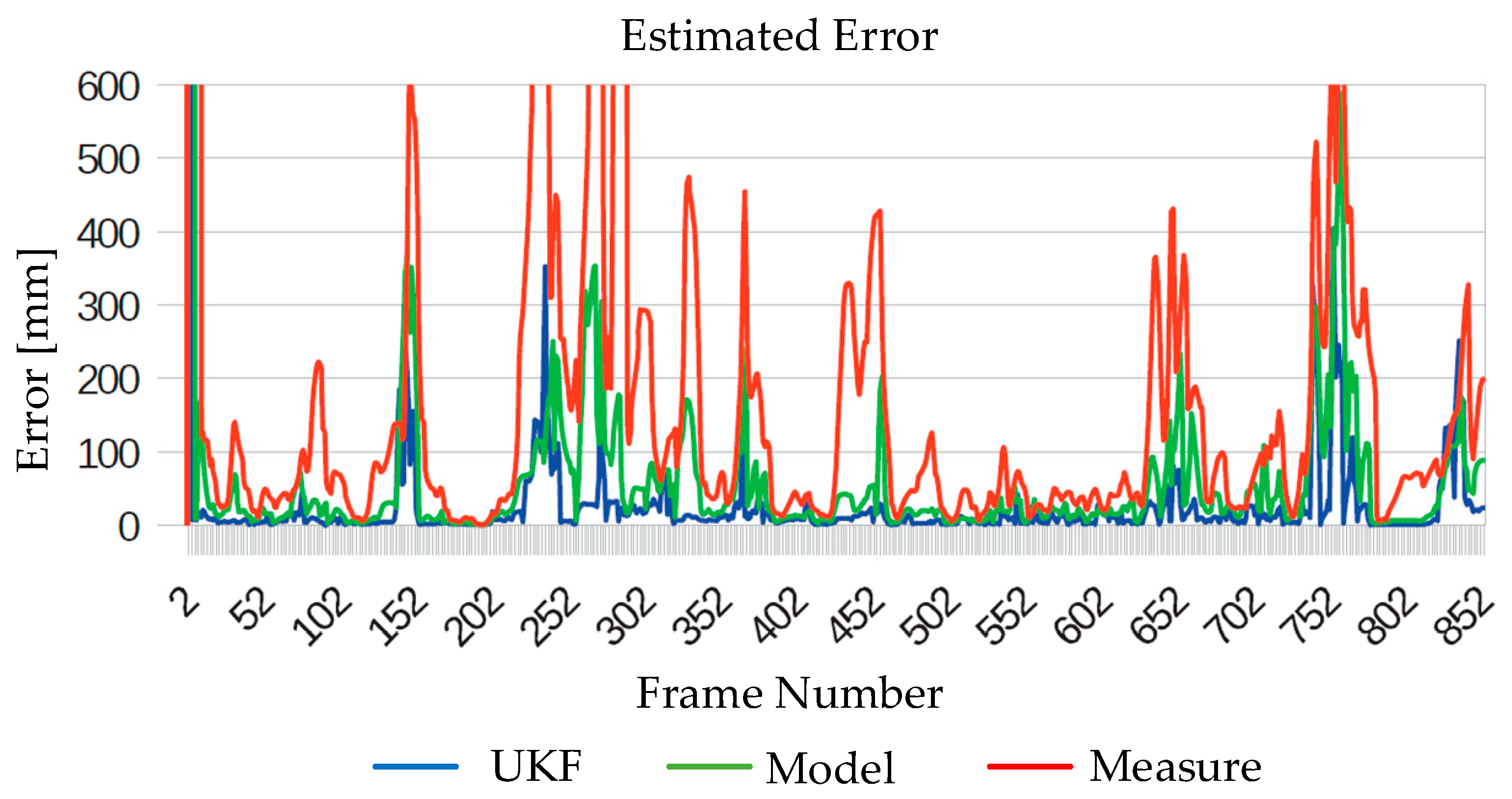
The UKF is used to enhance the robustness of the system. The UKF estimates the best road borders from the measurements in occlusion or in miss detection and presents a smooth road transition frame to frame.

(3)

The proposed system could be easily integrated with a local controller, such as pure pursuit, model predictive control (MPC) or Douglas-Peucker (DP). This will improve the navigation ability of robots in single lane road scenarios.

The rest of the paper is constructed as follows. Section 2 illustrates the related work of vision-based road detection. In Section 3, the mobile robot system is briefly introduced, including the description of the platform and system architecture. The specifications of the CCD camera used for road detection are listed in detail. Formulations of the road detection system and road tracking system are given at the end of this section. In Section 4, the road detection system is given in detail, such as the image processing module, color-based road detector and texture line detector. The UKF is used to fuse the detection results by the color-based and texture line detector and to track the target. We introduce the road tracking system that maps the road-following position in camera coordinate to world coordinate and calculates the control commands in Section 5, and we present our experiments in Section 6. Finally, the conclusions of this paper are given in Section 7.

2. Related Work

The vision sensors are defined as passive sensors and can be used for some specific applications, such as road detection, traffic sign recognition and obstacle identification [4]. Road detection is a fundamental issue in field robot navigation systems, which have attracted keen attention in the past several decades. As a result, various navigation algorithms for different types of vision sensors have been proposed [5,6,7,8]. Some of the works employ a monocular camera, stereo/multi camera, or depth camera systems for navigation. The road detection and target extraction are essential for vision-based navigation in outdoor environments. For these reasons, many state-of-the-art field robot systems employ vision sensors for road detection.

Xu et al. presented a mobile robot using a vision system to navigate in an unstructured environment [9]. The vision system consisted of two cameras. One is used for road region detection, and the other is used for road direction estimation. For a system trained by driving a robot through its environment, a vision-based road detection allows us to classify each individual image pixel as either an obstacle or the ground based on its color appearance [10]. For robot navigation in agricultural environments or hazardous related areas, a method for extracting and tracking man-made roads segments color images in small areas was proposed. These small areas are characterized later by color and texture attributes, and features are classified using the KNN rule or the Support Vector Machines method [4]. A vision-based road detection method was proposed to realize visual guiding navigation for autonomous land vehicles [11]. In this case, the images are segmented into road and non-road region using Otsu thresholding algorithm. Some methods detect road regions on triangular [12,13,14] or trapezoidal shape [15,16] and linear boundary constraints [17]. A triangle constraint means that the road surface is triangular in the image. In [12], one vanishing point and two road boundaries are detected to form a triangular road region. In [13], a self-supervised method is proposed, where positive and negative samples are initially extracted from the inside and outside of the triangle that corresponds to the road surface in the image. The road boundaries are fit to a trapezoidal model described by 5 parameters [16].

A number of deep learning-based methods for road surface segmentation have been proposed in recent years. A multitask deep convolutional network is developed for the problem of lane detection, which simultaneously detects the presence of the target and its geometric attributes with respect to the region of interest (ROI) [18]. Inspired by an iterative deep analysis thinking, a novel method is proposed to solve the optimal precision by balancing local and global information to conduct pixel-level classification for road segmentation [19]. A deep convolutional encoder-decoder architecture is proposed for semantic segmentation, termed SegNet [20]. SegNet performs competitively, achieving high scores for road scene understanding based on large and well-known datasets. However, end-to-end learning of deep segmentation architectures remains a challenge. In the literature ([15]), a symmetric and fixed-height trapezoid is used to reduce model parameters, and a single Gaussian model is used to describe the road surface. Yuan et al. proposed an online structural learning method, and the road boundary fitting is adopted to detect a more reliable boundary, while straight roads are assumed [17]. A vision-based control law is proposed to follow the road boundary with a monocular camera. This method is a part of the topological navigation to reduce prior information and enhance scalability of the map [21]. Although these methods seem to produce satisfactory results for pixel-wise scene segmentation, they require additional post-processing to determine the position of road marker images.

Although vision-based navigation techniques using cameras have been studied intensively for many years, no robots have achieved full camera navigation. An image acquired by the camera contains a large amount of information on the environments, such as color, shape, texture, distance and landmarks [22]. However, to extract useful information from the image and to make effective use of it is a long-standing problem. In addition, the lighting condition makes the problem even more difficult. Camera-based robots have to be tested thoroughly in outdoor environments for breakthrough purposes. A series of additional conjunct technologies have been developed for extracting environmental information [23], including semantic mapping, which provides an abstraction of space and a means for human-robot communication. Therefore, the formation of maps augmented by semasiology attributes involving human concepts, such as types of rooms, objects and their spatial arrangement, is considered a compulsory attribute for future robots that should be designed to operate in environments inhabited by humans. Semantic mapping could offer a qualitative description of the robot’s surroundings, aiming to augment the navigation capabilities.

3. Mobile Robot System

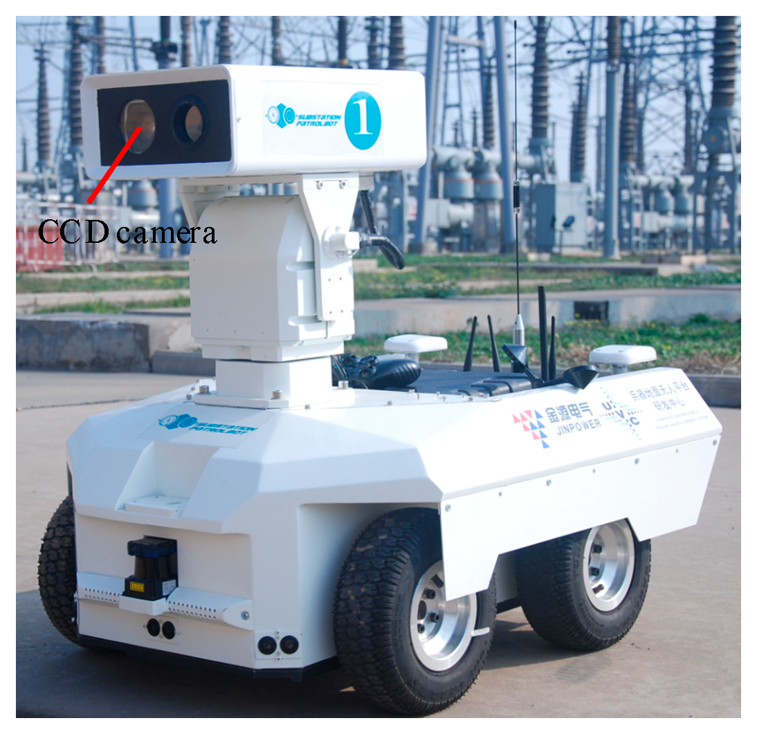
3.1. Platform Description

The mobile robot used for experiments in this study is a four-wheel driving system, which is equipped with a CCD camera, an on-board computer, a motion controller, wheel encoders and other devices, see Figure 1.

In order to capture the outside road view, a monocular network camera from HIK vision was used. The main specification of the camera and lenses is listed in

Table 1. The camera and lenses specifications.

Sensor type	HIK Vision DS-2ZCN2006 (C)
Resolution	1280 × 960
Format	JPEG or BMP
Frame rates	25 fps, 30 fps
Signal system	PAL/NTSC
Interface	1 RJ45 10 M/100 M Ethernet interface
Voltage requirements	DC12 V ± 10%
Power consumption	2.5 W (static), 4.5 W (dynamic)
Gain	0 to 16 DB
Shutter	1/1 s to 1/30,000 s
SNR	52 dB or better at minimum gain
Camera dimensions	74.3 mm × 81.1 mm × 142 mm
Mass	320 g
Operating temperature	−10 °C to 60 °C
Focal length	4.7–94 mm
Max CCD format	1/3″
Aperture	F1.6–F3.5
Maximum field of view	Horizontal: 58.9°
Video compression	H.265/H.264

. The on-board computer processes images from the CCD camera and computes the desired control commands to track the road-following waypoint. Then, it sends the control commands to the motion controller. The motion controller receives control commands from the computer and drives the robot to move.

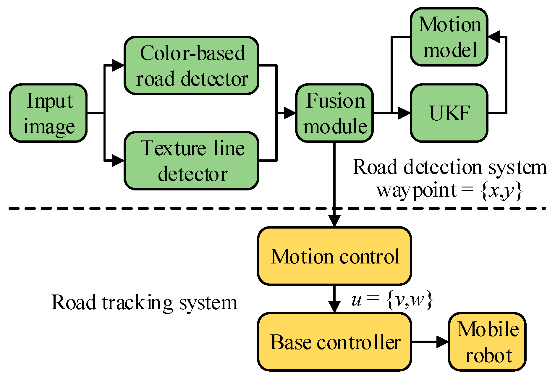
3.2. System Architecture

The system architecture consists of road detection system and road tracking system, see Figure 2. The overall system runs on the robot operating system (ROS) which provides a communication mechanism between different modules for the road-following system.

The road detection system is used to detect and track the border of unstructured roads, where the color-based road detector and texture line detector are implemented. Both methods work in parallel and are combined by a weighted average algorithm. The UKF is implemented to estimate and track the road borders. The final results of road detection system are the traversable road and the tracking waypoint on the road. The road tracking system is responsible for calculating the control commands and sending them to the robot base according to the tracking waypoint.

4. Road Detection System

The road detection system is divided into two components: a color-based road detector and a texture line detector. Both modules will detect the borders of the road using different approaches. One module uses color contrast, and the other module is based on texture. The borders detected by both modules are fused by a weighted average algorithm in the fusion module. The UKF is then implemented to track the road borders.

4.1. Image Processing Module

The image preprocessing process prepares the image in a state that makes it more effective to use in the algorithm. The raw image has undesirable characteristics that must be eliminated before use, for example, noise generated by the camera sensor, by the environment or by other factors. Another undesirable factor is the illumination that changes the properties of the image with different strength. First, the image is downsized to reduce the size and increase the processing speed. Then, a median filter is applied to reduce noise in the image, followed by white balance and RGB normalization to improve the image quality and reduce the illumination effects.

The original input image is 1280 × 960 pixels and is compressed to 640 × 480 pixels. The downsizing process is done by a nearest-neighbor interpolation, which means that a weighted average of pixels is performed in the nearest neighborhood. The scaling factor during the downsizing process is 2. Thus, the value of pixel (x, y) in the target image is set to the value of the pixel (x_o, y_o) in the original image, x_o = 2x, y_o = 2y. The objective of the downsizing is to cut the size of the image and reduce time consumption complexity in the following process.

In some cases, the focus of an algorithm is reduced to a small portion of the image because the other portion is meaningless. The image is reduced in size by taking account of the ROI. The ROI is extracted by cutting the image in the focus area and deleting the other part. This process enhances the time consumption, and by focusing only on the interest region, better results will be expected. The ROI is determined in an image according to vanishing points. In our system, the detection of vanishing point is based on literature [24], which presents a method for the automatic detection of vanishing points based on finding point alignments in a dual space, where converging lines in the image are mapped to aligned points. After the vanishing points are detected, the part of the image over it is eliminated, which corresponds to the skyline and horizon. Also, the bottom 1/5 of the image is excluded because that portion of the image corresponds to the frame of the robot; see Figure 3 as an example of image after ROI cropping. The ROI area can be adjusted depending on the location of the camera on the robot. The ROI parameters can be adjusted in configuration files.

The image contains only the region of interest after ROI is extracted. However, the noise is not eliminated in the image. Noise is a common effect due to the camera sensor and the procedure to convert the analogue 3D world to an image. A median filter is applied to reduce the impulse noise. A blur filter with a two-dimensional window, each one of size 7 × 7 pixels, is applied. For every pixel, the output values will be the median of the whole image pixel. After the filter is applied, the abrupt peaks values will be eliminated.

However, the illumination condition is changing all the time, since the robot is working in outdoor environments. The illumination condition is influenced by many factors, such as the intensity of sunlight that changes from time to time, or to the location of the camera related to sunlight that is not fixed; also, shadows can appear in the road, and so on. The white balance is adjusted and RGB normalization is performed to reduce the illumination effect. The white balance technique adjusts the intensities of colors taking into account the whole image. For each pixel in the image, the (R, G, B) value is calculated by using (1).

$$R^{\prime }=\frac{Y_{avg}}{R_{avg}},G^{\prime }=\frac{Y_{avg}}{G_{avg}},B^{\prime }=\frac{Y_{avg}}{B_{avg}}$$

(1)

in which $Y_{avg}$ is defined as $(R_{avg}+G_{avg}+B_{avg})/3$ and $R_{avg}$, $G_{avg}$, $B_{avg}$ are the average of $R$, $G$, $B$ channels.

RGB normalization is used to decrease distortions caused by illumination and to enhance results in color modelling after the white balance. For each pixel, the (R, G, B) value is updated by using (2).

$$R_{norm}=\frac{R}{rgb},G_{norm}=\frac{G}{rgb},B_{norm}=\frac{B}{rgb}$$

(2)

in which R, G, B are the red, green and blue channels, respectively, rgb is the sum of R, G, B for each pixel.

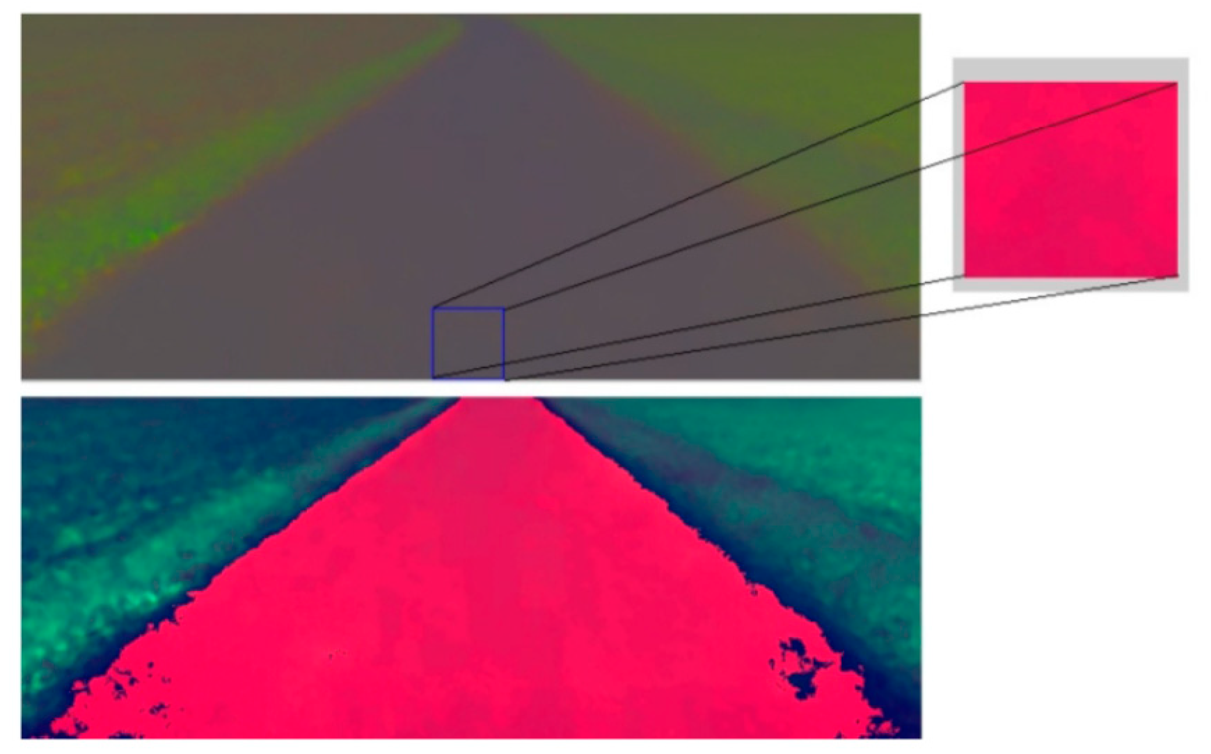
4.2. Color-Based Road Detector

The main features that are used to achieve a proper segmentation of the road image are the Hue and Saturation channels of the HSV color space. It has been shown that the Hue value is insensitive to shadows and water areas, which often cover parts of a road. The road color is extracted from each frame and used to classify each pixel. To extract the road color model, we assume that the road is in front of the camera. A small road area is extracted and it is transformed from RGB to HSV color space. The road window is located in the middle bottom of the image and has a size of 50 × 50 pixels. The middle bottom of the image is assumed to be road pixels; see Figure 4.

The segmentation of an image into an area associated with the road and into a non-road area is a rather crucial step. A mean-shift algorithm keeps track of the color model and establishes the segmentation criteria. The current prototype implements a road color model that is extracted frame by frame. This adaptation makes it more reliable and robust against changes in illumination or color. This adaptation is advantageous because avoids the requirement of prior knowledge of the road and allows road detection under different environmental circumstances; however, a disadvantage is that the wrong road model extraction would produce false road detection.

To avoid false road detection, we keep track of road color-histograms. The color model is adapted considering previous color models. The mean-shift tracking algorithm is an iterative scheme based on comparing the histogram of the road in the current image frame and histogram of the road color in previous image frames. The color model is updated by using (3).

$$C{M}_t=(1-\alpha )C{M}_{t-1}+\alpha CF$$

(3)

in which CM_t−1 is the previous road color model, CF is the road color model of the actual frame and α is 0.2 as a weight. Therefore, the proposed road color model is slow to adapt to a new road surface. A remembering process is applied in the sense that the contribution of a specific frame decreases exponentially the further it lies in the past.

The Manhattan distance classifies every pixel into a road or non-road area. Furthermore, the segmentation is enhanced with a hysteresis threshold that filters out some of the misjudgments. To reduce the computation complexity, not all pixels are used in the segmentation. Instead, pixels in non-consecutive rows and non-consecutive columns are selected. The distance of a pixel to the road model is evaluated by using (4).

$$Dist(i,j)=\frac{\left|H(i,j)-{\overline{q}}_{Hue}\right|+\left|S(i,j)-{\overline{q}}_{Sat}\right|}{2}$$

(4)

in which i and j are the pixels coordinates, H(i, j), S(i, j) are the Hue and Saturation values, respectively, and ${\overline{q}}_{Hue}$, ${\overline{q}}_{Sat}$ are the mean values of the road model in the Hue and Saturation channels.

The segmentation in the road and a non-road area is naturally affected by noise. A certain number of pixels will be misclassified; this is due to natural phenomena such as shadows, water areas, road texture, and obstacles. To reduce the noise, morphological filters (dilatation and erosion) are applied. The dilatation technique is used to fill up small noise holes, and erosion is used to eliminate disconnected line segments. The size of dilation or erosion kernel window is 3 × 3 pixels. In the case of multi-channel images, each channel is processed independently. To select the proper road borders, a rather trivial but effective heuristic technique is performed assuming that the road has parallel lines. With these procedures, obstacles and water areas on the road can be eliminated. This assumption states that the road width should decrease gradually from bottom to top due the perspective projection of the camera, and the middle line point of the road would not change suddenly because the road in the real world is continuous.

The above-mentioned color-based road detector is tested under a variety of light conditions and road scenarios; see Figure 5 for an example of road border detecting results. More road scene datasets and detection results are available at https://github.com/robotman801/roady.git.

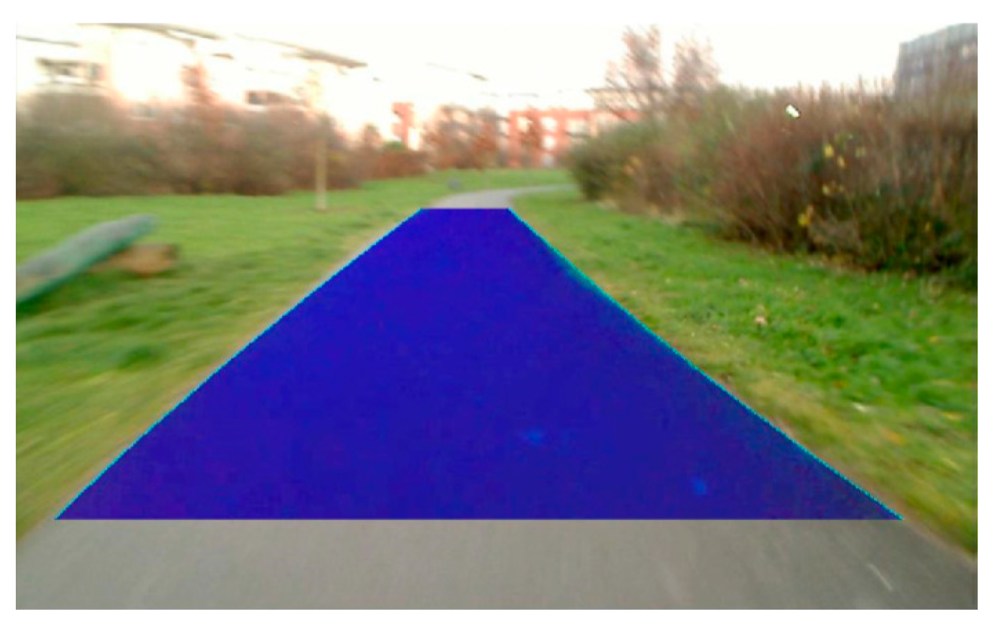
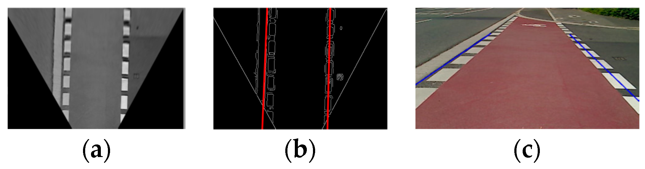
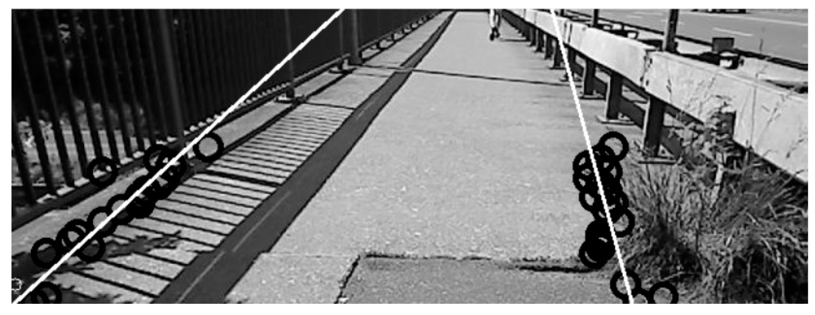
4.3. Texture Line Detector

The texture line detector does not require color contrast to detect a boundary. Instead, it is based on the texture or shape of the roads. This module detects straight lines in an inverse perspective mapping image (IPM). The IPM image is a change in the perspective, from the perspective of the camera to a top view of the road, see Figure 6. The IPM image has the benefit of eliminating the perspective distortions, which means that parallel lines that intersect in the vanishing point will appear again as parallel in the IPM image.

To obtain the IPM image, the camera intrinsic and extrinsic parameters are required to perform this transformation. The intrinsic parameters represent a projective transformation from the 3-D camera’s coordinates into the 2-D image coordinates. The extrinsic parameters represent a rigid transformation from the 3-D world coordinate system to the 3-D camera’s coordinate system. These parameters represent the rotation matrix and translation matrix between points in the camera’s coordinate system and world coordinate system.

• Intrinsic parameters are the parameters of the lens and the image sensor. These parameters consist of the camera focal lengths, the optical centers and also the distortion coefficients. The calibration algorithm detects the corners of a chessboard pattern. The chessboard pattern requires at least two snapshots. However, based on experience, more images produce better results. We used 24 images that cover the whole 3D visual area of the camera. The output of the algorithm is an “XML” file with the camera matrix and distortion coefficients.
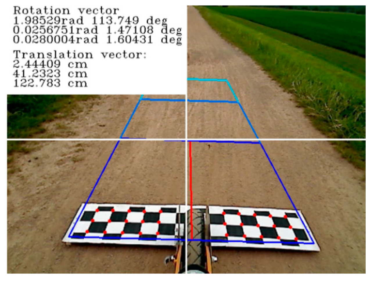
• Extrinsic parameters are calculated based on the Perspective-n-Point problem or PNP. This problem is used to estimate the position of an object when we have a calibrated camera. The locations of the 3D points on the object and the corresponding 2D projections in the image are known. The corresponding translation and rotation vectors can be estimated based on the 3D points and the corresponding 2D projections.

The camera parameters are computed from a chessboard pattern that is attached to the mobile robot, see Figure 7. The chessboard pattern is obstructed by the front tire of the mobile robot. The tire divides the pattern into two pieces. Therefore, the input image is divided into the left and the right side. On each side, 15 corner points are detected. The intrinsic parameters are calculated using the OpenCV library. The locations of the 3D points on the object and the corresponding 2D projections in the image are known. Thus, the corresponding translation and rotation vectors can be estimated based on the 3D points and the corresponding 2D projections, which are used as extrinsic parameters. This calibration process has to be done only once.

A canny edge detection algorithm is applied to the IPM image to detect vertical lines. Then, the clearly delineated edges are used within a Hough transform to detect the borders of the road. The Hough transform finds image features by collecting global evidence in a parameter space. In the most common application of the Hough transform, the features are lines and the parameters are their polar coordinates.

The vertical lines detected by the Hough transform are grouped into right and left depending on their location. For every group (Figure 8a,c), an outlier exclusion filter is applied to estimate the road borders. An example of the detected border is shown in Figure 8. The outlier exclusion criterion is a distance higher than two standard deviations of the line distribution.

4.4. Fusion Module with UKF

The borders detected by the color-based and the texture line detector are fused by a weighted average algorithm. From both modules, metrics are calculated to estimate a value of trust. The detected borders have more confidence and therefore a larger weight when the value of trust is high. The weight that every border will take is computed from metrics and it is updated in every cycle.

(1) Metrics of the color-based road detector

There is a fixed number of rows in every image, and we expect to find a border of the road in every row. The border is represented as a black circle in the following image; see Figure 9. The black circles are computed in the segmentation process. The trust value T_color of the color-based road detector is computed using (5).

$$T_{color}=\frac{\mathrm{Number}\mathrm{of}\mathrm{circles}\times 100}{2\times \mathrm{Number}\mathrm{of}\mathrm{rows}}$$

(5)

As indicated in (3), if the number of circles is the same as the number of rows in an image; the road is 100% detected in that image. Therefore, it will have a high trust value. On the other hand, if the number of circles is very low in an image, it means that the road is hardly detected. In this case, the trust value will be low, see Figure 10.

(2) Metrics of the texture line detector

After the IPM mapping and the canny edge detection, the Hough transform will compute the more likely vertical lines. These lines will be distributed over the image and will be grouped into left and right. The distribution of these lines will tell us the quality of the borders and therefore the trust value. Since the input image for line detection is the IPM image, which is scaled to 1 pixel (1 cm), the lines can have a maximum distribution of 320 pixels. Therefore, the line distribution means the number of lines that are detected by canny edge detection. The trust value T_texture of the texture line detector is computed by using (6). There will be two weights: one weight for the left border and the other one for the right border. Both weights are computed with (6).

$$T_{texture}=100\%-\frac{\mathrm{Lines}\mathrm{distribution}\times 100}{\mathrm{Number}\mathrm{of}\mathrm{columns}/2}$$

(6)

in which the number of columns is 640.

A greater distribution of the lines in the image will have a low trust value, and a small distribution of the lines will have a high trust value, see Figure 11.

After having computed the weights of the color-based road detector and texture line detector, the detection results are fused together. The fusion algorithm is a weighted average. The algorithm is expressed by using (7).

$$F=\beta \times \frac{T_{color}}{T_{color}+T_{texture}}+\gamma \times \frac{T_{texture}}{T_{color}+T_{texture}}$$

(7)

in which F is the fusion line, β is the color-based line, γ is the texture line.

The UKF is implemented to estimate and track the road borders. In the Kalman filter, two main steps rule the process. One is the measurement update step, where the measured signal is the combination of both modules, and a time update state, where the borders are estimated based on the motion model of the robot.

The estimation of the road borders is governed by the estimation of UKF [25]. The main idea behind the UKF is to obtain the best estimation of the borders from the measure and the movement of the robot. In the presented approach, the motion model of the lines is a non-linear function. It has been demonstrated that the UKF has a substantial performance gain in the context of state estimation for nonlinear systems compare with the Extended Kalman Filter (EKF). The UKF uses an unscented transformation to model non-linear dynamics, while the EKF will linearize the nonlinear system with the use of the Jacobian of the model; this linearization could cause divergence problems. In the presented approach, the borders of the road are represented by lines in a 2D Cartesian space. A line has two parameters, which are l and ψ. l represents the intersection point with the “x-axis” of the reference frame, and ψ represents the angle between the line and the “y-axis” of the reference frame; see Figure 12.

(1) The state

In the proposed approach, the left and the right borders will have an independent state, both of them have their own filter and will be computed separately. A state is represented as x = [l, ψ]. The state of the estimated line is represented as $\widehat{x}$ = [l⁻, ψ⁻], and ${\widehat{x}}^{-}$ is the last state of $\widehat{x}$.

(2) Measurement update

The state is updated based on the measurements by using (8).

$$\begin{array}{l}{K}_k=\frac{P_k^{-}}{(P_k^{-}+R_k)}\\ {\widehat{x}}_k={\widehat{x}}_k^{-}+K_k(z_k-{\widehat{x}}_k^{-})\\ P_k=(I-K_k)P_k^{-}\end{array}$$

(8)

in which the matrix R represents the covariance of the measurements. K is the Kalman gain that updates the ratio gain between the estimates and the measurements. The matrix P is the covariance error, and P⁻ is the covariance error of last period. The matrix R is updated in every step because the error variance of the measurements varies over time. The function z represents the process of detecting the road borders in the images.

(3) Time update

The function that models the movement of the lines will be represented by the function f (x_k−1, u_k−1, w_k−1). The function f relates the state x_k based on the previous state x_k−1, and the control input u_k−1 and w_k−1, which is the function that models the noise of the motion model. The motion model is a non-linear function that includes the homogeneous transformation which rotates and translates the lines based on the motion of the mobile robot $m(\phi ,\Delta x,\Delta y)$, where $\phi$ is the angle of difference of the robot between time steps, and $\Delta x$, $\Delta y$ are the displacements in the “x-axis” and “y-axis” respectively. The model also includes the transformation of lines from the polar to the corresponding Cartesian representation.

$$A=\left|\begin{array}{ccc}\cos \phi & -\sin \phi & \Delta x\\ \sin \phi & \cos \phi & \Delta y\\ 0& 0& 1\end{array}\right|$$

(9)

The Polar and Cartesian coordinates are related as:

$$\begin{array}{l}P(x,y)=(r\times \cos \phi ,r\times \sin \phi )\\ P(r,\phi )=(\sqrt{x^2+y^2},\arctan (y/x))\end{array}$$

(10)

Therefore, the time update is governed by:

$$\begin{array}{l}{\widehat{x}}_k^{-}=f({\widehat{x}}_{k-1},u_{k-1},w_{k-1})\\ P_k^{-}=P_{k-1}+Q_{k-1}\end{array}$$

(11)

in which the matrix Q represents the covariance of the motion model. It is updated in every step. It is updated based on the influence of the robot’s movement on the estimated line.

5. Road Tracking System

The road detection result is received from the road detection system described in Section 3, and can be represented simply as a bounding box at time t:

$${\mathbf{z}}_t={[u_t,v_t,w_t^{img},h_t^{img}]}^T$$

(12)

We assume that the ground is relatively flat, ignoring any in-plane rotation of the cylindrical object. For a pinhole camera with focal length f and principal point (c_x, c_y), we can write

$$\begin{array}{l}{u}_t=(f{x}_t^{cam}+c_x)/z_t^{cam}\\ v_t=(f{y}_t^{cam}+c_y)/z_t^{cam}\\ w_t^{img}=f{w}_0/z_t^{cam}\\ h_t^{img}=f{h}_0/z_t^{cam}\end{array}$$

(13)

in which (h₀, w₀) is the assumed road target’s height and width.

The rigid transformation of the center of the road target into the camera coordinate systems is homogeneously represented as

$${\mathrm{x}}_t^{cam}=\left[\begin{array}{c}{x}_t^{cam}\\ y_t^{cam}\\ z_t^{cam}\\ 1\end{array}\right]=T_t^{W/C}\left[\begin{array}{c}{x}_t\\ y_t\\ z_t\\ 1\end{array}\right]$$

(14)

in which $(x_t,y_t,z_t)$ is the road target’s position in the world coordinate and the transformation $T_t^{W/C}$ is defined as

$$T_t^{W/C}=T^{R/C}{T}_t^{W/R}$$

(15)

$T_t^{W/R}$ is the rigid transformation from the world coordinate system to the robot coordinate at time t, and $T^{R/C}$ is the fixed transformation from the robot coordinate system to the camera coordinate system. We can write

$$T_t^{W/R}=\left[\begin{array}{cc}{R}_t^T& -R_t^T{\mathbf{x}}_t^r\\ 0^T& 1\end{array}\right]$$

(16)

in which ${\mathbf{x}}_t^r=(x_t^r,y_t^r,z_t^r)$ and $R_t^T$ represent the orientation of the robot in the world coordinate frame, which can be obtained through the odometer and inertial measurement unit.

Hence, given the bounding box ${\mathbf{z}}_0$ of road detection, the initial position ${[x_0^{cam},y_0^{cam},z_0^{cam},1]}^T$ of the initial road target in the camera coordinate frame can be obtained by using (13). In (13), $x_0^{cam}$ and $y_0^{cam}$ can be calculated given $u_0$ if $z_0^{cam}$ is known. $z_0^{cam}$ can be obtained from $w_0^{img}$ or $h_0^{img}$, such as $z_0^{cam}=f{h}_0/h_0^{img}$. Then, the road target position at time 0 is mapped to the world coordinate frame by

$$\left[\begin{array}{c}{x}_0\\ y_0\\ z_0\\ 1\end{array}\right]={(T^{R/C}{T}_0^{W/C})}^{-1}\left[\begin{array}{c}{x}_0^{cam}\\ y_0^{cam}\\ z_0^{cam}\\ 1\end{array}\right]$$

(17)

For the given road detection bounding box ${\mathbf{z}}_t$ at time t, the corresponding road target position $(x_t,y_t,z_t)$ in the world coordinate frame can be calculated using (13) and (14) frame by frame.

After the road target position in the world coordinate is obtained, we treat it as the next tracking waypoint of the robot. The regular waypoint tracking controller can be integrated into the system to calculate the desired control commands, such as pure pursuit, MPC, and DP.

6. Experiments

The proposed road-following system is evaluated and tested on a variety of unstructured roads under different lighting and weather conditions. The condition includes both the environmental conditions as lighting and weather, and the structure condition like road material and border state. The system has also been tested under variable illumination. In this case, the same road has been surveyed with different lighting conditions during different hours on the same day, such as natural daylight, sunshine, sunset, etc.

The robot shown in Figure 1 is used for the road-following test in dynamic environments with maximum speed 0.5 m/s. More than 27,000 images are taking into account, which are grouped into 13 types of roads. During the image processing, the correct recognition is defined as a detection trust value higher than 90% according to (5) and (6). Hence, the correct rate is defined as the number of frames in which the road tracking position is recognized correctly over the total number of image frames. The statistical results of the experiment are listed in

Table 2. The correct rate.

Road Type Number	Characteristic	Number of Frames	Correct Rate
1	Bikeway, daylight, cement road	1912	97.8%
2	Parkway, sunset, cement road	734	97.4%
3	Parkway, daylight, asphalt road	3660	99.1%
4	Bikeway, sunset, asphalt road	1555	92.9%
5	Parkway, sunshine, asphalt road	951	95.7%
6	Bikeway, daylight, asphalt road	1645	99.39%
7	Parkway, daylight, dirt road	2123	99.15%
8	Sidewalk, daylight, brick road	4366	98.35%
9	Sidewalk, daylight, dirt road	3069	99.24%
10	Sidewalk, sunset, brick road	387	98.7%
11	Bikeway, sunshine, asphalt road	386	79.27%
12	Sidewalk, daylight, cement road	2066	99.61%
13	Sidewalk, daylight, asphalt road	1884	99.78%

. As shown in Table 2, the recognition rate median value is about 98.7%, with a minimum recognition rate of 79.27%. Therefore, the system has a recognition rate of 99.78% in the optimal case; in the regular cases, a recognition rate of about 98.7%; and in the worst cases, a recognition rate of 79.27%.

The image processing is run on a PC with an Intel Core i7 CPU at 2.93 GHz in Ubuntu 16.04. The software for image processing is written with C++ using OpenCV library. The proposed system works at the frame rate of 10 Hz. The computation time for each sub-process is clearly indicated in

Table 3. The required computation time for image processing.

Sub-Process	Time (ms)	Percentage (%)
Extraction of the region of interest	4.4915	6.03%
Smooth the image	0.47	0.63%
Apply white balance filter	10.31625	13.84%
Apply RGB normalization	5.6225	7.55%
Convert to HSV color space	2.70725	3.63%
Extraction of road window	0.403	0.54%
Image color segmentation	1.4385	1.93%
Morphological filtering	3.4315	4.61%
Border validation	0.457	0.61%
Road border estimation	1.17075	1.57%
IPM	11.79625	15.83%
Extraction of straight lines	12.57375	16.88%
Fusion of color-based borders and texture borders	9.503	12.76%
UKF computation	5.16875	6.94%
Draw IPM lines, 3D points and Kalman borders	4.951	6.65%
Total computation time [ms]	74.5

.

The runtimes are analyzed based on more than 24,700 images. The required computation time for image processing is shown in Table 3. The values that are shown in the column “Time (ms)” represent the average value of each sub-process during the road following. The column “Percentage (%)” shows the percentage of each sub-process in relation to the complete detection process.

As can be seen in Table 3, the sub-processes that require longer run times are the extraction of straight lines and the IPM. The extraction of the road image and the borders validation are the faster ones. The entire runtime required to processes one single image is about 74.5 ms. In other words, the value represents a frame rate of about 13.4 Hz. According to literature [20], the deep fully convolutional neural network SegNet for road scene segmentation needs more computational resources and trains much more slowly. The computational time of the forward pass and backward pass for SegNet architecture is 422.50 ms and 488.71 ms, respectively, i.e., a higher time cost than the image processing of our proposed method.

A sequence of frames showing the detection and road tracking target is presented in Figure 13. The red lines are the estimated road borders. The black square is the road tracking target in the image.

In order to evaluate the performance of the proposed system, the variance error is compared based on the measured line, detected line and estimated UKF lines; see Figure 14 for an example of an experiment with asphalt road in a parkway under sunshine illumination. The red line is the error of the measured lines detected by the color-based module and the texture line detector. The green line is the error of robot’s motion model that varies with time, which is based in the accuracy of the robot’s odometer. The error of estimated UKF lines is shown as the blue line. As indicated in Figure 14, the filter keeps the inertia of the estimated state and filters the high variance of the measurements and the motion model. The maximum error of UKF lines is 352 mm, and the average error of UKF lines is 33.6 mm. As a conclusion, the UKF produces minimal error and more stable road detection and tracking target position, even in the frames where the road boundaries are occluded.

7. Conclusions

This paper presents a low-cost road-following system for mobile robots based on a monocular camera. The system is composed of a road detection system and road tracking system. The color-based road detector and texture line detector are implemented in the road detection system and are fused to improve the road detection performance. The two detection methods work in parallel and are combined by a weighted average. The UKF produce the best estimates of the detected target, and it filters out the noise of the measurements and produces the estimated borders when the road is occluded or discontinuous.

The road tracking system provides the tracking waypoints for the robot by mapping the target position in camera coordinate to the position in world coordinate. After the waypoint in the world coordinate is given, the regular waypoint tracking controller can be integrated into the road-following system to calculate the control commands, such as the pure pursuit algorithm, MPC algorithm, and DP algorithm.

According to the experiment, it is shown that the system is more suitable with single lane roads. The results show a recognition rate of about 98.7% in regular illumination condition and minor target tracking error within a variety of environments under various lighting conditions. However, the proposed system does not work well in the environment where the road borders are not well defined or the road borders are not in the field of view of the camera. Future work will introduce some deep learning algorithms to set the parameters in the proposed system, such as the parameters of Hough transform and the area of ROI or pixel segmentation, and will focus on improving the application in various environments.

References

1. Wurm, K.M.; Kummerle, R.; Stachniss, C.; Burgard, W. Improving robot navigation in structured outdoor environments by identifying vegetation from laser data. In Proceedings of the 2009 IEEE/RSJ International Conference on Intelligent Robots and System, St. Louis, MO, USA, 11–15 October 2009; pp. 1217–1222. [Google Scholar]
2. Gim, S.; Adouane, L.; Lee, S.; Derutin, J.P. Clothoids composition method for smooth path generation of car-like vehicle navigation. J. Intell. Robot. Syst. 2017, 88, 129–146. [Google Scholar] [CrossRef]
3. Ort, T.; Paull, L.; Rus, D. Autonomous vehicle navigation in rural environments without detailed prior maps. In Proceedings of the 2018 IEEE International Conference on Robotics and Automation, Brisbane, Australia, 21–25 May 2018; pp. 1–8. [Google Scholar]
4. Cervantes, G.A.; Devy, M.; Hernandez, A.M. Lane extraction and tracking for robot navigation in agricultural applications. In Proceedings of the 11th International Conference on Advanced Robotics, Coimbra, Portugal, 30 June–3 July 2003; pp. 816–821. [Google Scholar]
5. Jia, B.; Liu, R.; Zhu, M. Real-time obstacle detection with motion features using monocular vision. Vis. Comput. 2015, 31, 281–293. [Google Scholar] [CrossRef]
6. Hane, C.; Sattler, T.; Pollefeys, M. Obstacle detection for self-driving cars using only monocular cameras and wheel odometry. In Proceedings of the 2015 IEEE/RSJ International Conference on Intelligent Robots and Systems, Hamburg, Germany, 28 September–2 October 2015; pp. 5101–5108. [Google Scholar]
7. Zhang, Z.; Xu, H.; Chao, Z.; Li, X.; Wang, C. A novel vehicle reversing speed control based on obstacle detection and sparse representation. IEEE Trans. Intell. Transp. Syst. 2015, 16, 1321–1334. [Google Scholar] [CrossRef]
8. Maier, D.; Hornung, A.; Bennewitz, M. Real-time navigation in 3D environments based on depth camera data. In Proceedings of the 2012 IEEE-RAS International Conference on Humanoid Robots, Osaka, Japan, 29 November–1 December 2012; pp. 692–697. [Google Scholar]
9. Xu, W.; Zhuang, Y.; Hu, H.; Zhao, Y. Real-time road detection and description for robot navigation in an unstructured campus environment. In Proceedings of the 11th World Congress on Intelligent Control and Automation, Shenyang, China, 27–30 June 2014; pp. 928–933. [Google Scholar]
10. Ulrich, I.; Nourbakhsh, I. Appearance-based obstacle detection with monocular color vision. In Proceedings of the AAAI National Conference on Artificial Intelligence, Austin, TX, USA, 30 July–3 August 2000; pp. 866–871. [Google Scholar]
11. Wang, Y.; Cui, D.; Su, C.; Wang, P. Vision-based road detection by Monte Carlo Method. Inf. Technol. J. 2010, 9, 481–487. [Google Scholar] [CrossRef]
12. Kong, H.; Audibert, J.Y.; Ponce, J. Vanishing point detection for road detection. In Proceedings of the IEEE Conference on Computer Vision and Pattern Recognition, Miami Beach, FL, USA, 20–25 June 2009; pp. 96–103. [Google Scholar]
13. Zhou, S.; Iagnemma, K. Self-supervised learning method for unstructured road detection using fuzzy support vector machines. In Proceedings of the IEEE/RSJ International Conference on Intelligent Robots and Systems, Taipei, Taiwan, 18–22 October 2010; pp. 1183–1189. [Google Scholar]
14. Wang, Q.; Fang, J.; Yuan, Y. Adaptive road detection via context-aware label transfer. Neurocomputing 2015, 158, 174–183. [Google Scholar] [CrossRef]
15. Ososinski, M.; Labrosse, F. Automatic driving on Ill-defined roads: An adaptive, shape-constrained, color-based method. J. Field Robot. 2013, 32, 504–533. [Google Scholar] [CrossRef]
16. Jeong, H.; Oh, Y.; Part, J.H.; Koo, B.S.; Lee, S.W. Vision based adaptive and recursive tracking of unpaved roads. Pattern Recognit. Lett. 2002, 23, 73–82. [Google Scholar] [CrossRef]
17. Yuan, Y.; Jiang, Z.; Wang, Q. Video-based road detecting via online structural learning. Neurocomputing 2015, 168, 336–347. [Google Scholar] [CrossRef]
18. Li, J.; Mei, X.; Prokhorov, D. Deep neural network for structural prediction and lane detection in traffic scene. IEEE Trans. Neural Netw. Learn. Syst. 2016, 99, 1–14. [Google Scholar] [CrossRef] [PubMed]
19. Chen, X.; Qiao, Y. Road segmentation via iterative deep analysis. In Proceedings of the IEEE International Conference on Robotics and Biomimetics, Zhuhai, China, 6–9 December 2015; pp. 2640–2645. [Google Scholar]
20. Badrinarayanan, V.; Kendall, A.; Cipolla, R. SegNet: A deep convolutional encoder-decoder architecture for scene segmentation. IEEE Trans. Pattern Anal. Mach. Intell. 2017, 39, 2481–2495. [Google Scholar] [CrossRef] [PubMed]
21. Kurashiki, K.; Aguilar, M.; Soontornvanichkit, S. Visual navigation of a wheeled mobile robot using front image in semi-structured environment. J. Robot. Mechatron. 2015, 27, 392–400. [Google Scholar] [CrossRef]
22. Agrawal, M.; Konolige, K.; Bolles, R. Localization and mapping for autonomous navigation in outdoor terrains: A stereo vision approach. In Proceedings of the IEEE Workshop Applications of Computer Vision, Austin, TX, USA, 21–22 February 2007; p. 7. [Google Scholar]
23. Kostavelis, I.; Gasteratos, A. Semantic mapping for mobile robotics tasks: A survey. Robot. Auton. Syst. 2015, 66, 86–103. [Google Scholar] [CrossRef]
24. Lezama, J.; Randall, G.; Grompone, R. Vanishing point detection in urban scenes using point alignments. Image Process. On Line 2017, 7, 131–164. [Google Scholar] [CrossRef]
25. Julier, S.; Uhlmann, J. A new extension of the kalman filter to nonlinear systems. In Proceedings of the 11th International Symposium on Aerospace/Defence Sensing, Simulation and Controls, Orlando, FL, USA, 11 April 1997; pp. 182–193. [Google Scholar]
Figure 1. Robot platform.
Applsci 08 01635 g001
Figure 2. Structure diagram of the vision-based road-following system.
Applsci 08 01635 g002
Figure 3. Image after ROI cropping.
Applsci 08 01635 g003
Figure 4. Road window located in the middle bottom of size 50 × 50 pixels.
Applsci 08 01635 g004
Figure 5. Road detected by the color-based road detector.
Applsci 08 01635 g005
Figure 6. Inverse perspective mapping. (a) Original image; (b) Image after IPM transformation.
Applsci 08 01635 g006
Figure 7. Computed camera parameters from the pattern in the image.
Applsci 08 01635 g007
Figure 8. Texture line detector. (a) IPM image. (b) Lines obtained from the Hough transform after canny edge detector. (c) Detected road borders.
Applsci 08 01635 g008
Figure 9. Black circles are used to compute the metrics.
Applsci 08 01635 g009
Figure 10. Road borders with low confidence value.
Applsci 08 01635 g010
Figure 11. Lines used to compute the metrics. Left lines (orange), high distribution, low confidence. Right lines (green), low distribution, high confidence.
Applsci 08 01635 g011
Figure 12. Line parametrization.
Applsci 08 01635 g012
Figure 13. Road detection and target position of sequence frames. Estimated road borders (red). 2 × 5 m grid (green). Road tracking target position (black square). (a) Sidewalk; (b) Bikeway; (c) Parkway; (d) Parkway with sunset.
Applsci 08 01635 g013
Figure 14. Comparison of the error of the estimated UKF with the errors of the motion model and the measure mode.
Applsci 08 01635 g014