Ownership Cost Comparison of Battery Electric and Non-Plugin Hybrid Vehicles: A Consumer Perspective


Abstract
1. Introduction
2. Materials and Methods
2.1. Study Design, Setting, & Data
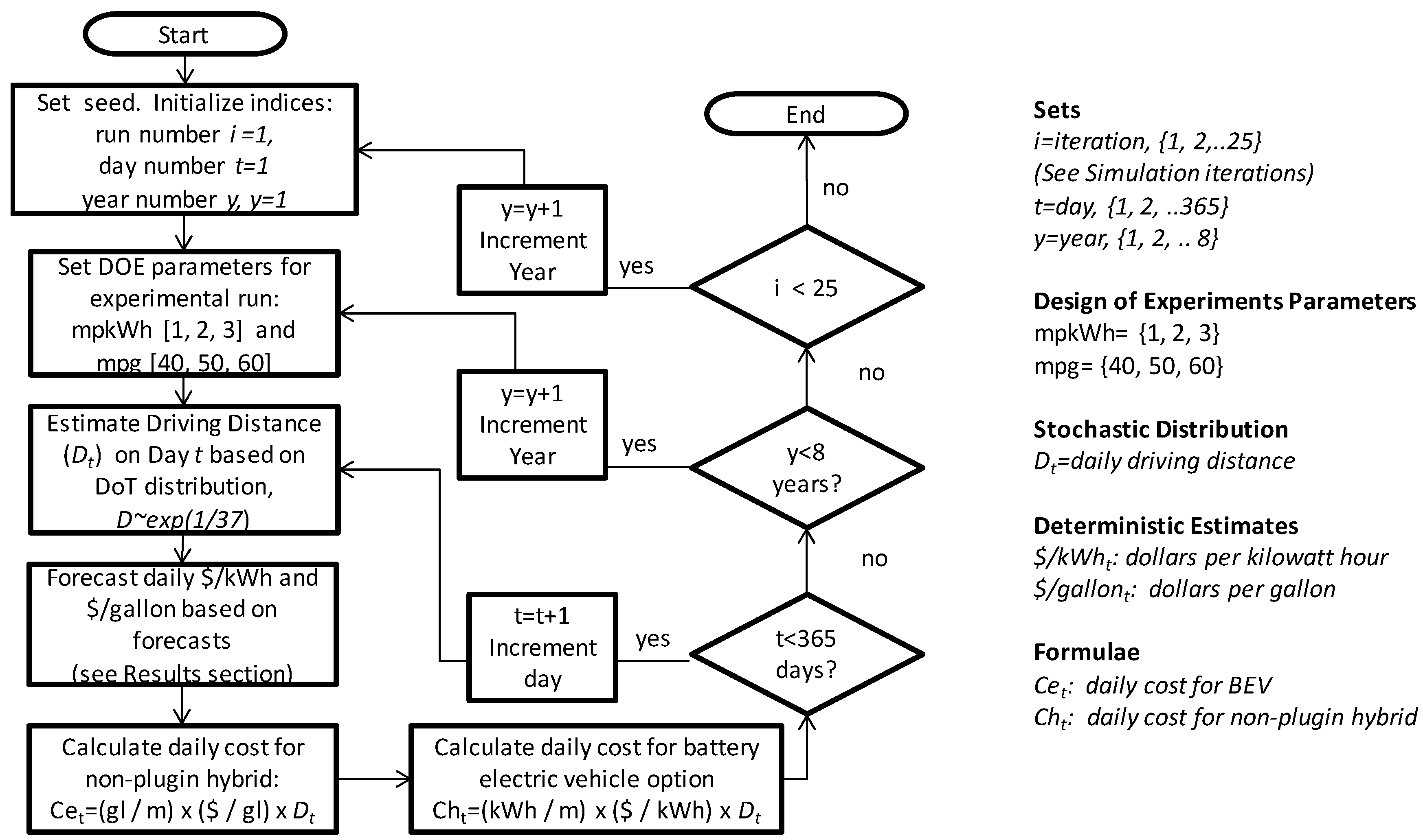
2.2. Simulation Sets, Parameters, Stochastic Variables, Deterministic Variables, Formulae, and Flowcharts
3. Results
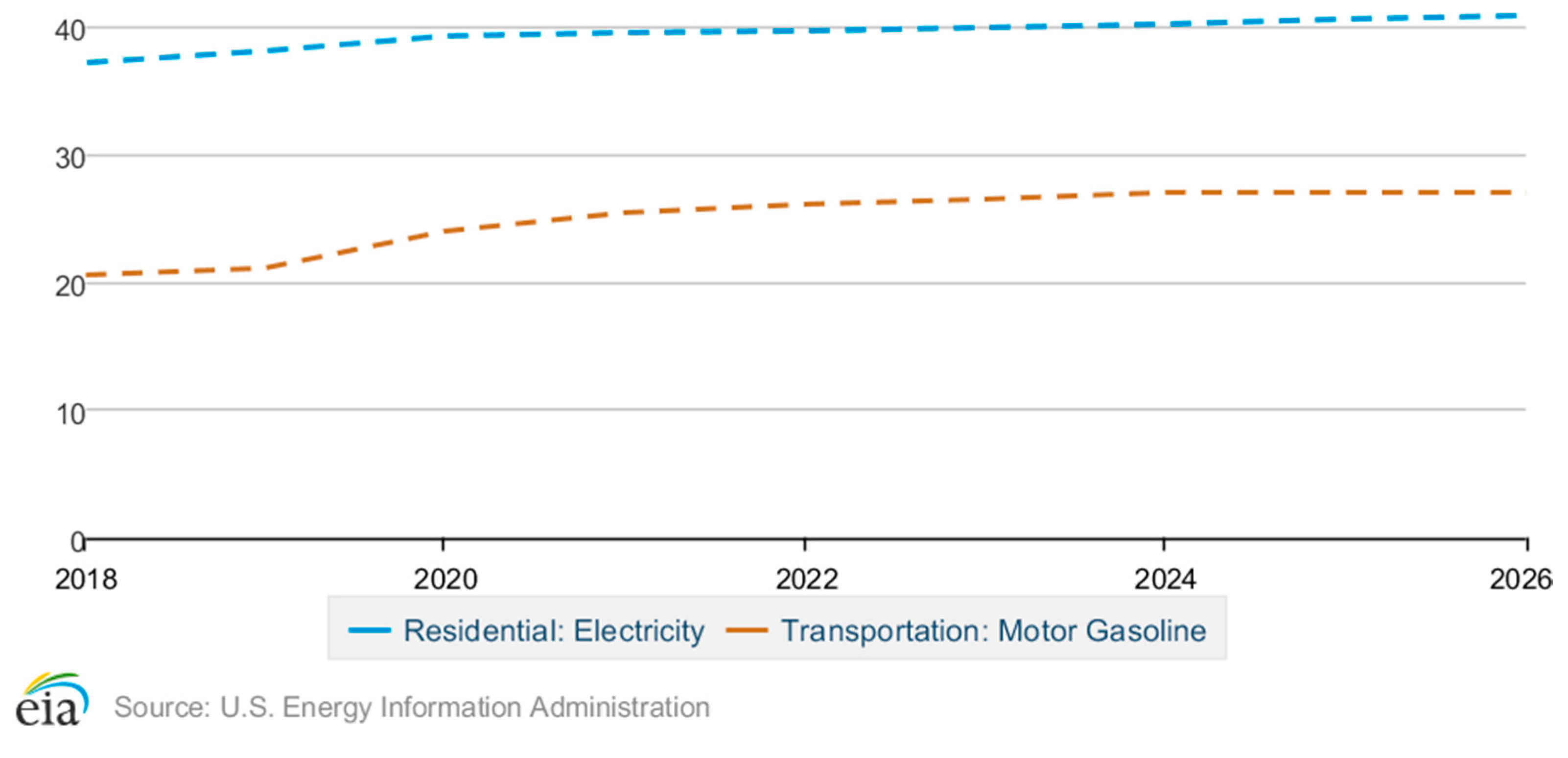
3.1. Descriptive Statistics
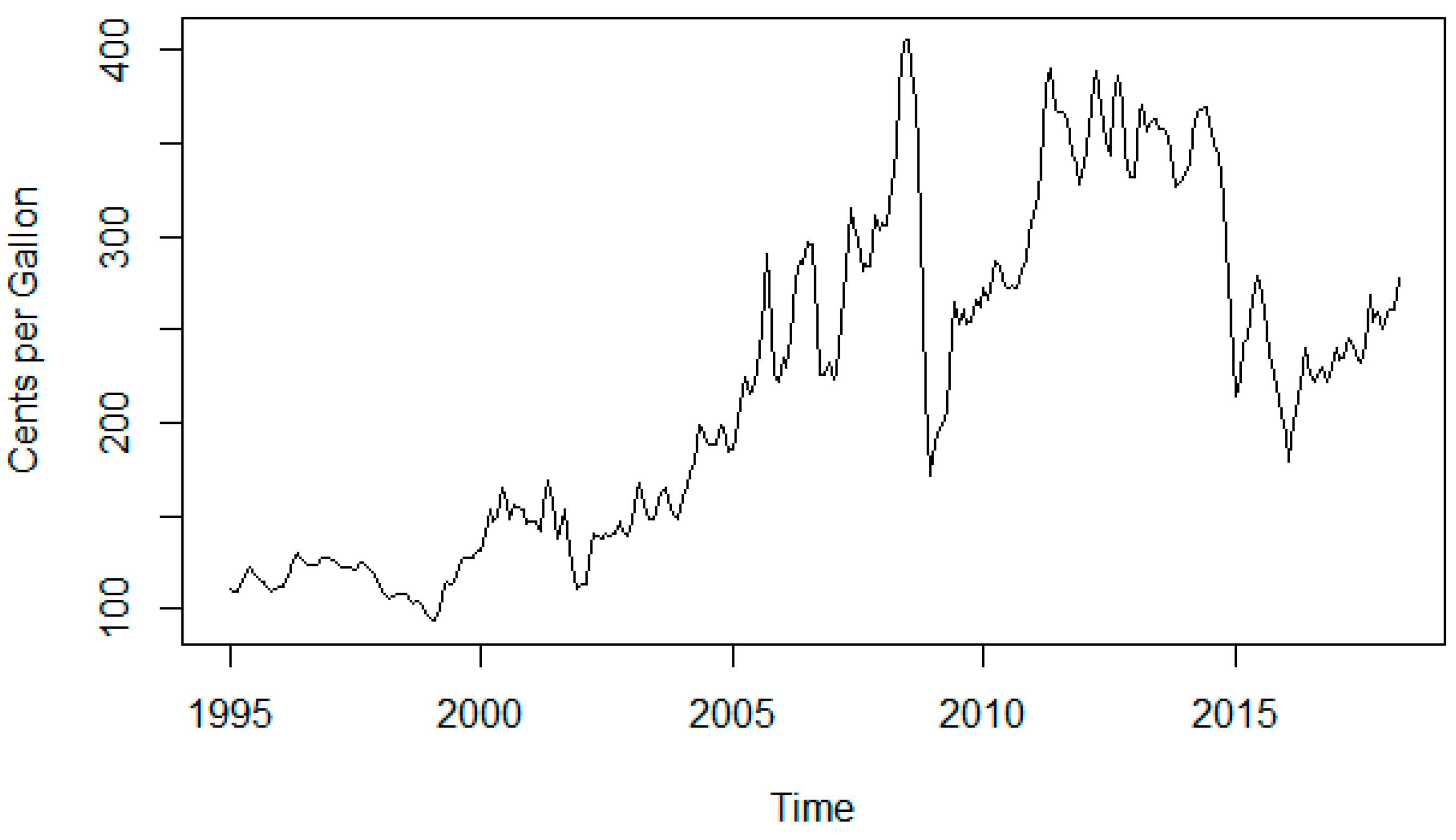
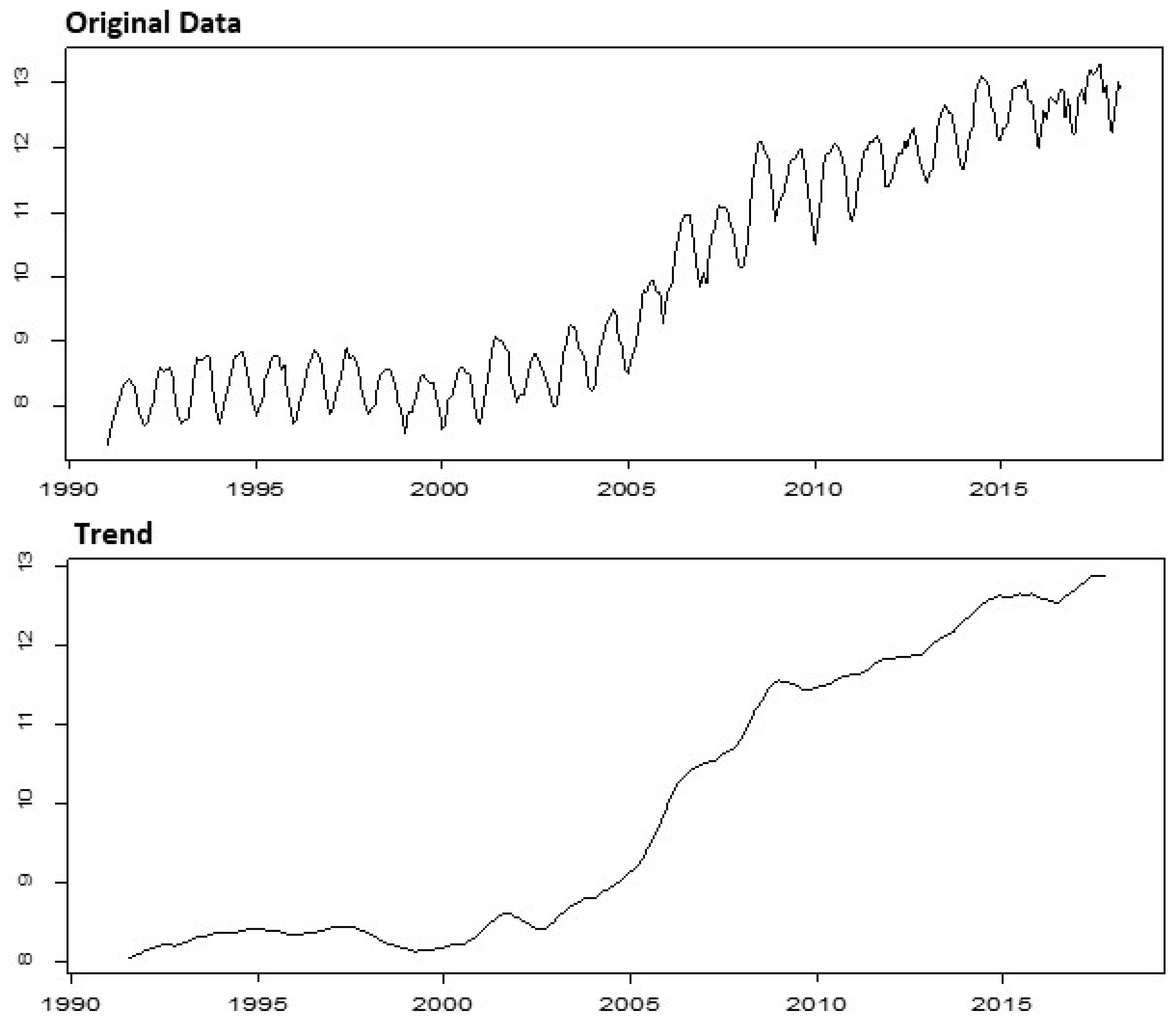
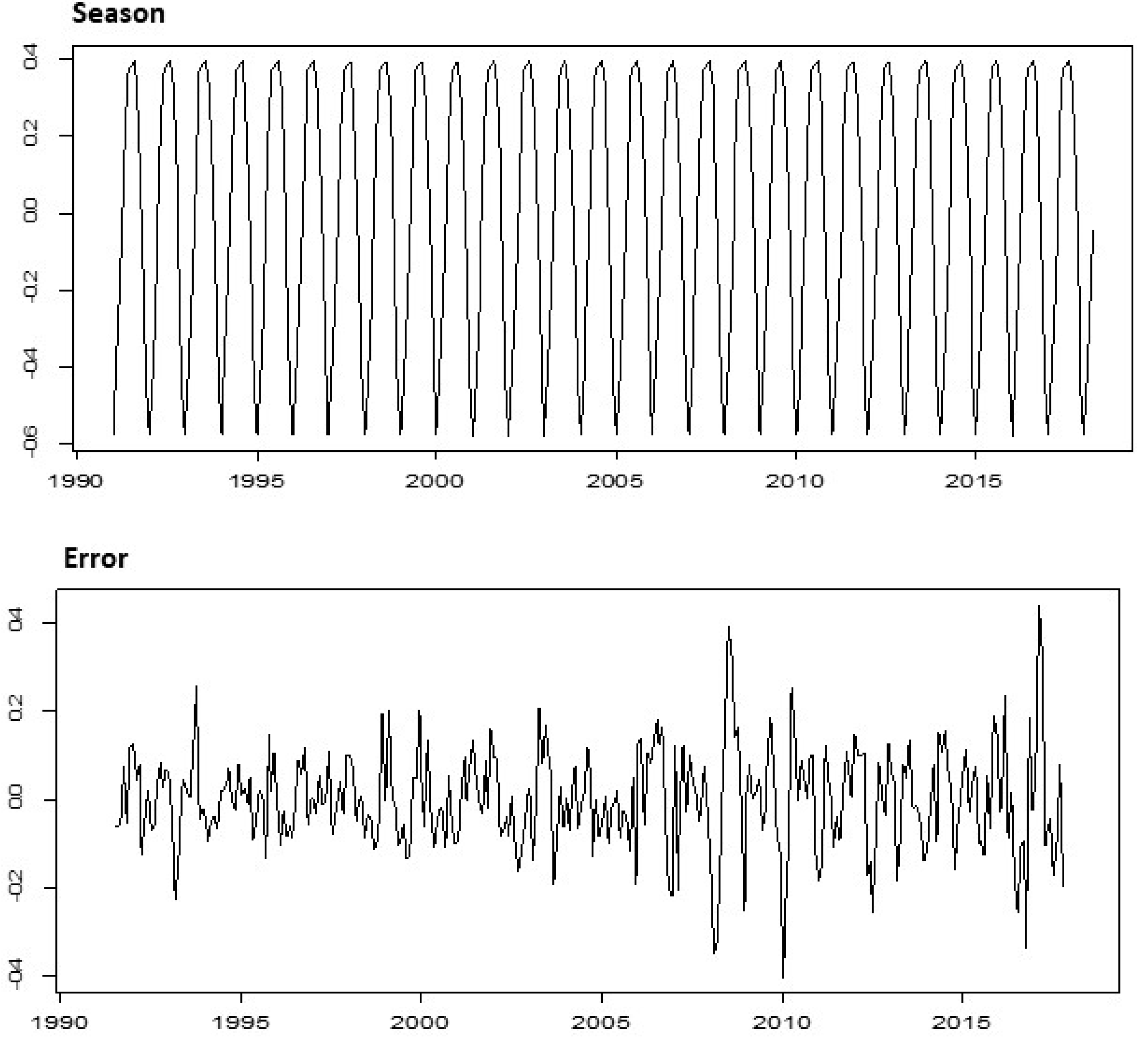
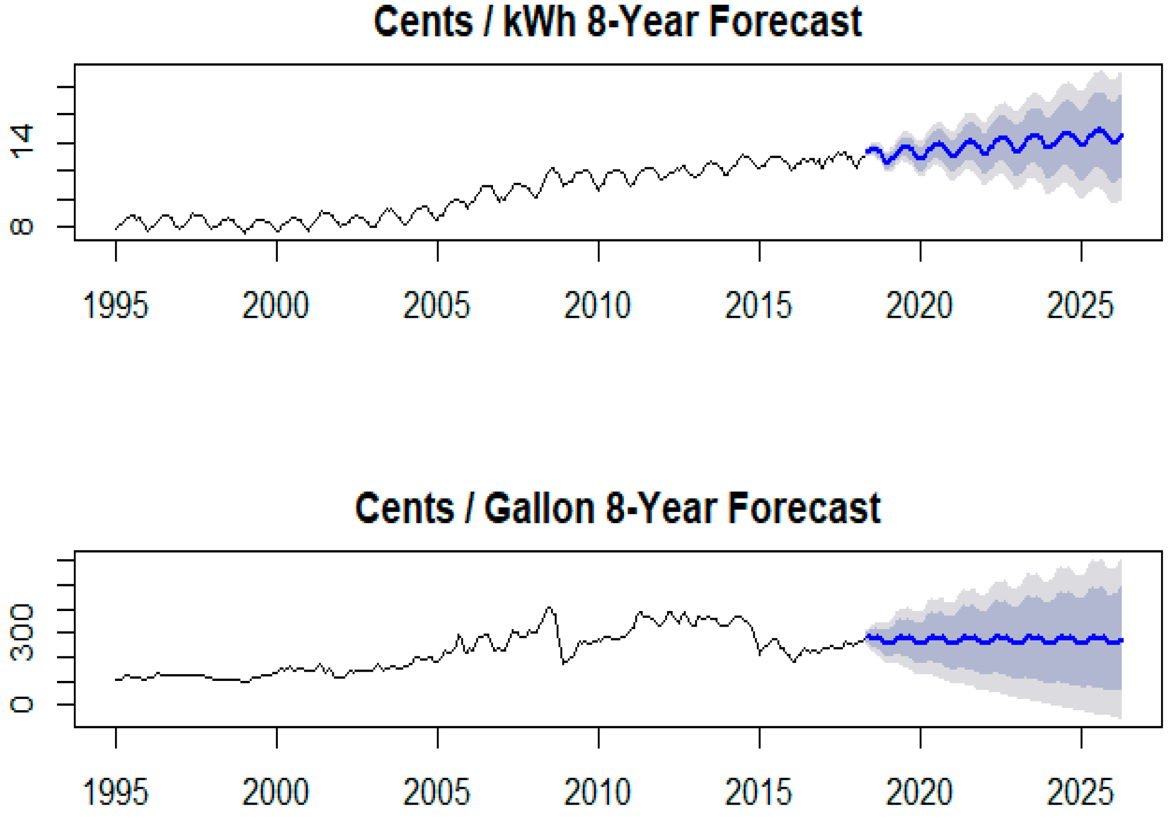
3.2. Forecasts
3.3. Daily Driving Distribution
3.4. Simulation Iterations
3.5. Verification and Validation
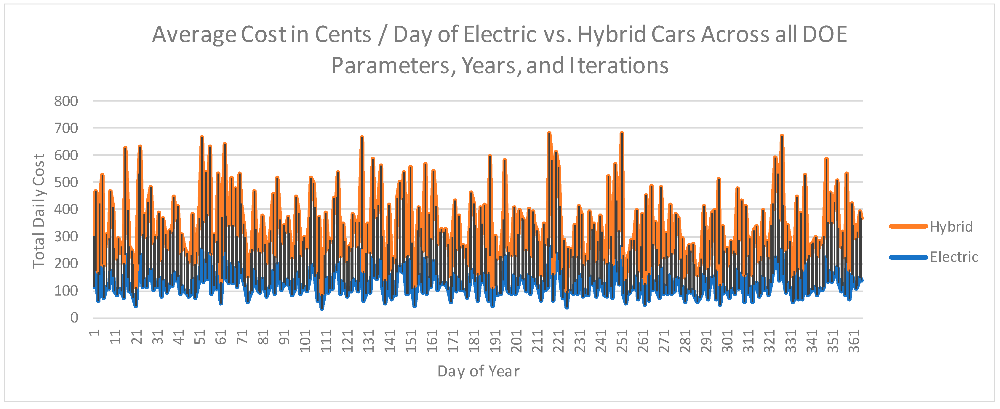
3.6. Simulation Results
4. Discussion
Funding
Conflicts of Interest
References
- Fulton, L.; Bastian, N. A Fuel Cost Comparison of Electric and Gas-Powered Vehicles. In Proceedings of the 2012 AutumnSim Conference on Energy, Climate and Environmental Modeling & Simulation, San Diego, CA, USA, 28–31 October 2012. [Google Scholar]
- Hagman, J.; Ritzén, S.; Stier, J.J.; Susilo, Y. Total cost of ownership and its potential implications for battery electric vehicle diffusion. Res. Transp. Bus. Manag. 2016, 18, 11–17. [Google Scholar] [CrossRef]
- Delucchi, M.A.; Lipman, T.E. An analysis of the retail and lifecycle cost of battery-powered electric vehicles. Transp. Res. Part D Trans. Environ. 2001, 6, 371–404. [Google Scholar] [CrossRef]
- Lipman, T.E.; Delucchi, M.A. A retail and lifecycle cost analysis of hybrid electric vehicles. Transp. Res. Part D 2006, 11, 115–132. [Google Scholar] [CrossRef]
- Silva, C.; Farias, T.; Ross, M. Evaluation of energy consumption, emissions and cost of plug-in hybrid vehicles. Energy Convers. Manag. 2009, 50, 1635–1643. [Google Scholar] [CrossRef]
- Werber, M.; Fischer, M.; Schwartz, P.V. Batteries: Lower cost than gasoline? Energy Policy 2009, 37, 2465–2468. [Google Scholar] [CrossRef]
- Weiller, C. Plug-in hybrid electric vehicle impacts on hourly electricity demand in the United States. Energy Policy 2011, 39, 3766–3778. [Google Scholar] [CrossRef]
- Ernst, C.S.; Hackbarth, A.; Madlener, R.; Lunz, B.; Sauer, D.U.; Eckstein, L. Battery sizing for serial plug-in hybrid electric vehicles: A model-based economic analysis for Germany. Energy Policy 2011, 39, 5871–5882. [Google Scholar] [CrossRef]
- Al-Alawi, B.M.; Bradley, T.H. Total cost of ownership, payback, and consumer preference modeling of plug-in hybrid electric vehicles. Appl. Energy 2013, 103, 488–506. [Google Scholar] [CrossRef]
- Wu, G.; Inderbitzin, A.; Bening, C. Total cost of ownership of electric vehicles compared to conventional vehicles: A probabilistic analysis and projection across market segments. Energy Policy 2015, 80, 196–214. [Google Scholar] [CrossRef]
- Lieven, T.; Mühlmeier, S.; Henkel, S.; Waller, J.F. Who will buy electric cars? An empirical study in Germany. Transp. Res. Part D 2011, 16, 236–243. [Google Scholar] [CrossRef]
- Shin, J.; Hong, J.; Jeong, G.; Lee, J. Impact of electric vehicles on existing car usage: A mixed multiple discrete–continuous extreme value model approach. Transp. Res. Part D 2012, 17, 138–144. [Google Scholar] [CrossRef]
- He, L.; Chen, W.; Conzelmann, G. Impact of vehicle usage on consumer choice of hybrid electric vehicles. Transp. Res. Part D 2012, 17, 208–214. [Google Scholar] [CrossRef]
- Kelly, J.C.; MacDonald, J.S.; Keoleian, G.A. Time-dependent plug-in hybrid electric vehicle charging based on national driving patterns and demographics. Appl. Energy 2012, 94, 395–405. [Google Scholar] [CrossRef]
- Özdemir, E.D. Impact of electric range and fossil fuel price level on the economics of plug-in hybrid vehicles and greenhouse gas abatement costs. Energy Policy 2012, 46, 185–192. [Google Scholar] [CrossRef]
- Ahmadi, P.; Cai, X.M.; Khanna, M. Multicriterion optimal electric drive vehicle selection based on lifecycle emission and lifecycle cost. Int. J. Energy Res. 2018, 42, 1496–1510. [Google Scholar] [CrossRef]
- Palmer, K.; Tate, J.E.; Wadud, Z.; Nellthorp, J. Total cost of ownership and market share for hybrid and electric vehicles in the UK, US and Japan. Appl. Energy 2018, 209, 108–119. [Google Scholar] [CrossRef]
- U.S. Department of Energy. Electricity. Available online: https://www.eia.gov/electricity/data.php (accessed on 21 July 2018).
- U.S. Department of Energy. Petroleum and Other Liquids. Available online: https://www.eia.gov/petroleum/ (accessed on 21 July 2018).
- U.S. Department of Transportation, Federal Highway Administration. 2017 National Household Travel Survey. 2017. Available online: https://nhts.ornl.gov/vehicle-miles (accessed on 21 July 2018).
- Google.com. Available online: www.google.com (accessed on 21 July 2018).
- LeBeau, P. Americans Holding onto Their Cars Even Longer. 2015. Available online: https://www.cnbc.com/2015/07/28/americans-holding-onto-their-cars-longer-than-ever.html (accessed on 21 July 2018).
- Voelker, J. Electric Car Batteries Compared. Green Car Reports. 2016. Available online: https://www.greencarreports.com/news/1107864_electric-car-battery-warranties-compared (accessed on 21 July 2018).
- Berman, B. Total Cost of Ownership of an Electric Car. 2016. Available online: plugincars.com (accessed on 21 July 2018).
- Vogan, M. Electric Vehicle Residual Value Outlook. 2017. Available online: https://www.moodysanalytics.com/-/media/presentation/2017/electric-vehicle-residual-value-outlook.pdf (accessed on 21 July 2018).
- EVAdoption.com. EV Statistics of the Week: Range, Price and Battery Size of Currently Available (in the US) BEVs. Available online: http://evadoption.com/ev-statistics-of-the-week-range-price-and-battery-size-of-currently-available-in-the-us-bevs/ (accessed on 21 July 2018).
- Department of Energy. Fueleconomy.gov. 2018. Available online: https://www.fueleconomy.gov/feg/PowerSearch.do?action=alts&path=3&year1=2017&year2=2018&vtype=Electric&srchtyp=newAfv (accessed on 21 July 2018).
- U.S. Department of Transportation. Average Annual Miles per Driver per Year Group. 2018. Available online: https://www.fhwa.dot.gov/ohim/onh00/bar8.htm (accessed on 21 July 2018).
- Pepitone, J. Gas Prices Fall below $1.87. 2018. Available online: https://money.cnn.com/2008/11/26/news/economy/gas_prices_sink/index.htm?postversion=2008112612 (accessed on 21 July 2018).
- Samuelson, R. Key Facts about the Great Oil Bust of 2014. The Washington Post, 3 December 2014. [Google Scholar]
- U.S. Department of Energy. Annual Energy Outlook. 2018. Available online: https://www.eia.gov/outlooks/aeo/ (accessed on 16 August 2018).
- Hyndman, R. Forecasting Principles & Practice, 2nd ed.; OTexts: Melbourne, Australia, 2013; Available online: https://otexts.org/fpp2/ (accessed on 28 August 2018).
- R Core Team. R: A Language and Environment for Statistical Computing; R Foundation for Statistical Computing: Vienna, Austria, 2018. [Google Scholar]
- AAA Foundation for Traffic Safety. American Driving Survey. 2015–2016. Available online: http://aaafoundation.org/american-driving-survey-2015-2016/ (accessed on 21 July 2018).


| Manufacturer | Make | Range in Miles | kWh Battery Pack | Miles/kWh | MSRP Base |
|---|---|---|---|---|---|
| BMW | i3 | 114 | 33 | 3.45 | $44,450.00 |
| Fiat | 500e | 87 | 24 | 3.63 | $32,995.00 |
| Ford | Focus Electric | 115 | 33 | 3.48 | $29,120.00 |
| Chevrolet | Bolt EV | 238 | 60 | 3.97 | $36,620.00 |
| Honda | Clarity Electric | 89 | 25.5 | 3.49 | $33,400.00 |
| Hyundai | Ioniq Electric | 124 | 28 | 4.43 | $29,500.00 |
| Kia | Soul EV | 111 | 30 | 3.70 | $32,250.00 |
| Nissan | Leaf | 107 | 30 | 3.57 | $29,990.00 |
| Tesla | Model 3 | 310 | 78 | 3.97 | $35,000.00 |
| Tesla | Model S 75D | 275 | 75 | 3.67 | $74,500.00 |
| Tesla | Model S 100D | 351 | 100 | 3.51 | $94,000.00 |
| Tesla | Model S P100D | 337 | 100 | 3.37 | $135,000.00 |
| Tesla | Model X 75 | 237 | 75 | 3.16 | $70,532.00 |
| Tesla | Model X 100D | 295 | 100 | 2.95 | $96,000.00 |
| Model XP100 | Model X P100D | 289 | 100 | 2.89 | $140,000.00 |
| VW | e-Golf | 125 | 35.8 | 3.49 | $30,495.00 |
| Make | Model | Engine Size (All 4 Cylinder Automatics) | Estimated mpg | MSRP |
|---|---|---|---|---|
| Hyundai | Ioniq Blue | 1.6 L | 58 | $22,200.00 |
| Toyoto | Prius Eco | 1.8 L | 56 | $25,165.00 |
| Hundai | Ioniq | 1.6 L | 55 | $22,000.00 |
| Toyota | Camry Hybrid LE | 2.5 L | 52 | $27,950.00 |
| Toyota | Prius | 1.8 L | 52 | $23,475.00 |
| Kia | Niro FE | 1.6 L | 50 | $23,340.00 |
| Kia | Niro | 1.6 L | 49 | $23,340.00 |
| Honda | Accord Hybrid | 2.0 L | 47 | $25,100.00 |
| Chevrolet | Malibu Hybrid | 1.8 L | 46 | $27,920.00 |
| Toyota | Camry Hybrid LXE | 2.5 L | 46 | $32,400.00 |
| Toyota | Prius c | 1.5 L | 46 | $20,630.00 |
| ME | RMSE | MAE | MPE | MAPE | MASE | |
|---|---|---|---|---|---|---|
| ETS Gasoline | 0.450 | 13.096 | 8.538 | 0.082 | 3.835 | 0.235 |
| ARIMA Gasoline | 0.666 | 12.689 | 8.802 | 0.220 | 3.881 | 0.242 |
| ETS kWh | 0.004 | 0.133 | 0.102 | 0.043 | 0.990 | 0.355 |
| ARIMA kWH | 0.003 | 0.134 | 0.103 | 0.043 | 0.995 | 0.358 |
| n = 365 Days | Mean for 3 mpkWh | Mean for 4 mpkWh | Mean for 5 mpkWh | Mean for 40 mpg | Mean for 50 mpg | Mean for 60 mpg |
|---|---|---|---|---|---|---|
| Mean | $1.58 | $1.19 | $0.95 | $2.46 | $1.97 | $1.64 |
| Std. Error | $0.03 | $0.02 | $0.02 | $0.05 | $0.04 | $0.03 |
| Median | $1.46 | $1.10 | $0.88 | $2.29 | $1.83 | $1.53 |
| Std. Dev. | $0.58 | $0.44 | $0.35 | $0.91 | $0.72 | $0.60 |
| Range | $2.91 | $2.18 | $1.75 | $ 4.45 | $3.56 | $2.97 |
| Minimum | $0.44 | $0.33 | $0.26 | $0.68 | $0.54 | $0.45 |
| Maximum | $3.35 | $2.51 | $2.01 | $5.13 | $4.10 | $3.42 |
| Make | Model | Type | MSRP Base | Fuel $ | Tax Credits | Maintenance | Insur-ance | Residual | Ownership Costs |
|---|---|---|---|---|---|---|---|---|---|
| Hyundai | Ioniq Electric | Electric | $29,500.00 | $3173.00 | $7500.00 | $3781.40 | $11,800.00 | $5605.00 | $35,148.90 |
| Toyota | Prius c | Hybrid | $20,630.00 | $5859.00 | - | $6482.40 | $8252.00 | $5982.70 | $35,240.49 |
| Ford | Focus Electric | Electric | $29,120.00 | $4073.00 | $7500.00 | $3781.40 | $11,648 | $5532.80 | $35,589.25 |
| Hundai | Ioniq | Hybrid | $22,000.00 | $4866.00 | - | $6482.40 | $8800.00 | $6380.00 | $35,768.77 |
| Hyundai | Ioniq Blue | Hybrid | $22,200.00 | $4819.00 | - | $6482.40 | $8880.00 | $6438.00 | $35,942.90 |
| Nissan | Leaf | Electric | $29,990.00 | $3969.00 | $7500.00 | $3781.40 | $11,996.00 | $5698.10 | $36,537.82 |
| VW | e-Golf | Electric | $30,495.00 | $4061.00 | $7500.00 | $3781.40 | $12,198.00 | $5794.05 | $37,241.43 |
| Toyota | Prius | Hybrid | $23,475.00 | $4914.00 | - | $6482.40 | $9390.00 | $6807.75 | $37,453.88 |
| Kia | Niro FE | Hybrid | $23,340.00 | $5744.00 | - | $6482.40 | $9336.00 | $6768.60 | $38,133.71 |
| Kia | Niro | Hybrid | $23,340.00 | $5773.00 | - | $6482.40 | $9336.00 | $6768.60 | $38,162.43 |
| Kia | Soul EV | Electric | $32,250.00 | $3818.00 | $7500.00 | $3781.40 | $12,900.00 | $6127.50 | $39,122.01 |
| Toyoto | Prius Eco | Hybrid | $25,165.00 | $4850.00 | - | $6482.40 | $10,066.00 | $7297.85 | $39,265.96 |
| Fiat | 500e | Electric | $32,995.00 | $3899.00 | $7500.00 | $3781.40 | $13,198.00 | $6269.05 | $40,104.45 |
| Honda | Accord Hybrid | Hybrid | $25,100.00 | $5830.00 | - | $6482.40 | $10,040.00 | $7279.00 | $40,173.47 |
| Tesla | Model 3 | Electric | $35,000.00 | $3506.00 | $7500.00 | $3781.40 | $14,000.00 | $6650.00 | $42,137.12 |
| Toyota | Camry Hybrid LE | Hybrid | $27,950.00 | $4914.00 | - | $6482.40 | $11,180.00 | $8105.50 | $42,421.13 |
| Chevrolet | Malibu Hybrid | Hybrid | $27,920.00 | $5859.00 | - | $6482.40 | $11,168.00 | $8096.80 | $43,332.39 |
| Chevrolet | Bolt EV | Electric | $36,620.00 | $3506.00 | $7500.00 | $3781.40 | $14,648.00 | $6957.80 | $44,097.32 |
| Honda | Clarity Electric | Electric | $33,400.00 | $4061.00 | Lease Only | $3781.40 | $13,360.00 | $6346.00 | $48,256.48 |
| Toyota | Camry Hybrid LXE | Hybrid | $32,400.00 | $5859.00 | - | $6,482.40 | $12,960.00 | $9396.00 | $48,305.19 |
| BMW | i3 | Electric | $44,450.00 | $4107.00 | $7500.00 | $3781.40 | $17,780.00 | $8445.50 | $54,173.26 |
| Tesla | Model X 75 | Electric | $70,532.00 | $4443.00 | $7500.00 | $3781.40 | $28,212.00 | $13,401.08 | $86,068.01 |
| Tesla | Model S 75D | Electric | $74,500.00 | $3853.00 | $7500.00 | $3781.40 | $29,800.00 | $14,155.00 | $90,279.22 |
| Tesla | Model S 100D | Electric | $94,000.00 | $4038.00 | $7500.00 | $3781.40 | $37,600.00 | $17,860.00 | $114,059.34 |
| Tesla | Model X 100D | Electric | $96,000.00 | $4859.00 | $7500.00 | $3781.40 | $38,400.00 | $18,240.00 | $117,300.81 |
| Tesla | Model S P100D | Electric | $135,000.00 | $4200.00 | $7500.00 | $3781.40 | $54,000 | $25,650.00 | $163,831.32 |
| Tesla | Model X P100D | Electric | $140,000.00 | $5137.00 | $7500.00 | $3781.40 | $56,000 | $26,600.00 | $170,818.49 |
| Make | Model | Type | MSRP Base | Fuel $ | Tax Credits | Maintenance | Residual | Ownership Costs |
|---|---|---|---|---|---|---|---|---|
| Hyundai | Ioniq Electric | Electric | $29,500.00 | $3172.50 | $7500.00 | $3781.40 | $5605.00 | $23,348.90 |
| Ford | Focus Electric | Electric | $29,120.00 | $4072.65 | $7500.00 | $3781.40 | $5532.80 | $23,941.25 |
| Nissan | Leaf | Electric | $29,990.00 | $3968.52 | $7500.00 | $3781.40 | $5698.10 | $24,541.82 |
| VW | e-Golf | Electric | $30,495.00 | $4061.08 | $7500.00 | $3781.40 | $5794.05 | $25,043.43 |
| Kia | Soul EV | Electric | $32,250.00 | $3818.11 | $7500.00 | $3781.40 | $6127.50 | $26,222.01 |
| Fiat | 500e | Electric | $32,995.00 | $3899.10 | $7500.00 | $3781.40 | $6269.05 | $26,906.45 |
| Hundai | Ioniq | Hybrid | $22,000.00 | $4866.37 | - | $6482.40 | $6380.00 | $26,968.77 |
| Toyota | Prius c | Hybrid | $20,630.00 | $5858.79 | - | $6482.40 | $5982.70 | $26,988.49 |
| Hyundai | Ioniq Blue | Hybrid | $22,200.00 | $4818.50 | - | $6482.40 | $6438.00 | $27,062.90 |
| Toyota | Prius | Hybrid | $23,475.00 | $4914.23 | - | $6482.40 | $6807.75 | $28,063.88 |
| Tesla | Model 3 | Electric | $35,000.00 | $3505.72 | $7500.00 | $3781.40 | $6650.00 | $28,137.12 |
| Kia | Niro FE | Hybrid | $23,340.00 | $5743.91 | - | $6482.40 | $6768.60 | $28,797.71 |
| Kia | Niro | Hybrid | $23,340.00 | $5772.63 | - | $6482.40 | $6768.60 | $28,826.43 |
| Toyoto | Prius Eco | Hybrid | $25,165.00 | $4850.41 | - | $6482.40 | $7297.85 | $29,199.96 |
| Chevrolet | Bolt EV | Electric | $36,620.00 | $3505.72 | $7500.00 | $3781.40 | $6957.80 | $29,449.32 |
| Honda | Accord Hybrid | Hybrid | $25,100.00 | $5830.07 | - | $6482.40 | $7279.00 | $30,133.47 |
| Toyota | Camry Hybrid LE | Hybrid | $27,950.00 | $4914.23 | - | $6482.40 | $8105.50 | $31,241.13 |
| Chevrolet | Malibu Hybrid | Hybrid | $27,920.00 | $5858.79 | - | $6482.40 | $8096.80 | $32,164.39 |
| Honda | Clarity Electric | Electric | $33,400.00 | $4061.08 | Lease Only | $3781.40 | $6346.00 | $34,896.48 |
| Toyota | Camry Hybrid LXE | Hybrid | $32,400.00 | $5858.79 | - | $6482.40 | $9396.00 | $35,345.19 |
| BMW | i3 | Electric | $44,450.00 | $4107.36 | $7500.00 | $3781.40 | $8445.50 | $36,393.26 |
| Tesla | Model X 75 | Electric | $70,532.00 | $4442.89 | $7500.00 | $3781.40 | $13,401.08 | $57,855.21 |
| Tesla | Model S 75D | Electric | $74,500.00 | $3852.82 | $7500.00 | $3781.40 | $14,155.00 | $60,479.22 |
| Tesla | Model S 100D | Electric | $94,000.00 | $4037.94 | $7500.00 | $3781.40 | $17,860.00 | $76,459.34 |
| Tesla | Model X 100D | Electric | $96,000.00 | $4859.41 | $7500.00 | $3781.40 | $18,240.00 | $78,900.81 |
| Tesla | Model S P100D | Electric | $135,000.00 | $4199.92 | $7500.00 | $3781.40 | $25,650.00 | $109,831.32 |
| Tesla | Model X P100D | Electric | $140,000.00 | $5137.09 | $7500.00 | $3781.40 | $26,600.00 | $114,818.49 |
© 2018 by the author. Licensee MDPI, Basel, Switzerland. This article is an open access article distributed under the terms and conditions of the Creative Commons Attribution (CC BY) license (http://creativecommons.org/licenses/by/4.0/).
Share and Cite
Fulton, L. Ownership Cost Comparison of Battery Electric and Non-Plugin Hybrid Vehicles: A Consumer Perspective. Appl. Sci. 2018, 8, 1487. https://doi.org/10.3390/app8091487
Fulton L. Ownership Cost Comparison of Battery Electric and Non-Plugin Hybrid Vehicles: A Consumer Perspective. Applied Sciences. 2018; 8(9):1487. https://doi.org/10.3390/app8091487
Chicago/Turabian StyleFulton, Lawrence. 2018. "Ownership Cost Comparison of Battery Electric and Non-Plugin Hybrid Vehicles: A Consumer Perspective" Applied Sciences 8, no. 9: 1487. https://doi.org/10.3390/app8091487
APA StyleFulton, L. (2018). Ownership Cost Comparison of Battery Electric and Non-Plugin Hybrid Vehicles: A Consumer Perspective. Applied Sciences, 8(9), 1487. https://doi.org/10.3390/app8091487