A Baseline for General Music Object Detection with Deep Learning

Abstract

Deep learning is bringing breakthroughs to many computer vision subfields including Optical Music Recognition (OMR), which has seen a series of improvements to musical symbol detection achieved by using generic deep learning models. However, so far, each such proposal has been based on a specific dataset and different evaluation criteria, which made it difficult to quantify the new deep learning-based state-of-the-art and assess the relative merits of these detection models on music scores. In this paper, a baseline for general detection of musical symbols with deep learning is presented. We consider three datasets of heterogeneous typology but with the same annotation format, three neural models of different nature, and establish their performance in terms of a common evaluation standard. The experimental results confirm that the direct music object detection with deep learning is indeed promising, but at the same time illustrates some of the domain-specific shortcomings of the general detectors. A qualitative comparison then suggests avenues for OMR improvement, based both on properties of the detection model and how the datasets are defined. To the best of our knowledge, this is the first time that competing music object detection systems from the machine learning paradigm are directly compared to each other. We hope that this work will serve as a reference to measure the progress of future developments of OMR in music object detection.

1. Introduction

Optical Music Recognition (OMR) is the field of research that investigates how to computationally read music notation in documents. Having accurate OMR technology would enable fully integrating written music into the ecosystem of digital music processing. In recent years, diverse initiatives have been launched to digitize musical heritage in the written form, such as the The Digital Image Archive of Medieval Music project [1] on the academic side, or at the same time the crowd-sourced International Music Score Library Project (IMSLP) repository of public-domain and openly available music [2] which has grown to become a primary provider of sheet music worldwide. However, making not only the digital images of all these compositions, but also their structured representation accessible at scale, as attempted e.g., by the Single Interface for Music Score Searching and Analysis (SIMSSA) project [3], would constitute a breakthrough in interacting with written music, and making it accessible to both the professional and the general public in previously unseen ways: content-based search in large sheet music libraries including cross-modal retrieval, digital musicology at scale and with access to structured representations of music that only exists in written form, renotation of early notation to modern notation, manuscript transcription and part-matching to directly cut costs of music directors and composers. These (and more) applications have been envisioned in OMR literature for a long time [4,5]; however, results have not been forthcoming [6].

In order to be able to apply Music Information Retrieval (MIR) algorithms on music scores and enable this wide range of applications, it is first necessary to bring them into this symbolic, machine-readable format. Manually creating such symbolic representations by means of specialized music typesetting software is an expensive effort, and constitutes the bottleneck to digitally encoding music at large scales—which is, in turn, a bottleneck both for digital musicology, subsequent MIR applications, and music accessibility.

OMR is expected to provide the enabling technology for scalable structured encoding. From this perspective, OMR can be seen as the key to diversifying the available symbolic music sources in reasonable time and cost. Crucially, OMR has seen a shift in paradigms in the last few years, mainly triggered by advances in the field of computer vision and machine learning through deep learning [7,8,9,10]. This development is further fueled by the availability of large annotated datasets (e.g., MUSCIMA++, DeepScores) and sufficient computational power to work with such large datasets. This new paradigm, combined with a better understanding of the challenges [11,12], allow approaching the problem of OMR somewhat differently.

The entire process of OMR can be broken down into the following steps [6,13,14,15]:

• Preprocessing: Standard techniques to ease further steps, e.g., contrast enhancement, binarization, skew-correction or noise removal. Additionally, the layout should be analyzed to allow subsequent steps to focus on actual content and ignore the background.
• Music Object Detection: This step is responsible for finding and classifying all relevant symbols or glyphs in the image. Note that music object detection is sometimes referred to as music symbol recognition, but we use the former term because of its relation to “object detection”, which is commonly used in computer vision to refer to the very same localization and classification task in (natural) images, answering the question “What is where in this image?”.
• Relational Understanding: From the detected and classified symbols, a music notational graph (MuNG) can be constructed that holds both the symbols and their relationships to each other. Note that, for a complete and unambiguous reconstruction, two kinds of relations are necessary: a logical relationship (e.g., between a notehead and a stem) and a temporal relationship to guarantee the correct order of the symbols. The graph formulation essentially re-casts the notation reconstruction algorithms like that of [16] as a problem of recovering binary labels over symbol pairs, therefore also making it amenable to machine learning approaches. Again, other works sometimes refer to the stage after object detection as semantical reconstruction. Note that, in this approach, this stage only attempts to reconstruct the relations between symbols and a large part of the semantics is assigned in the encoding stage.
• Encoding: Given a complete music notation graph, the music can be encoded into any output format unambiguously, e.g., into MIDI for playback or MusicXML/MEI for further editing in a music notation program. Keep in mind that this step potentially has to deal with the subtleties of music notation, such as omitted symbols.

Currently, the hardest challenge of this pipeline is posed by the music object detection step. Unfortunately, it is unclear to what extent deep learning has been successful in addressing this stage. Existing studies that focus on music notation objects are dispersed and not comparable with each other in terms of the used algorithms, datasets, and metrics, which has so far made a fair comparison impossible. However, there is no good reason for this state of affairs: music object detection can borrow standard evaluation from generic object detection settings, and the deep learning models are similarly domain-agnostic. Therefore, this work aims to fill an obvious gap: provide a direct comparison between the different general deep learning models for object detection that were recently proposed for the task of music object detection, across the available musical symbol datasets, and thus establish a clear state-of-the-art baseline.

We evaluate three competing approaches on three distinct datasets containing both handwritten and typeset music. To compare the different approaches on common ground, we propose a standard bounding-box based data model, usable with multiple OMR datasets, and use an up-to-date standard for evaluating object detection, namely the Common Objects in Context (COCO) evaluation protocol [17]. All scripts for obtaining the test-bed, preprocessing the data and evaluating the results are being made publicly available [18].

To the best of our knowledge, this marks the first time that music object detection methods based on machine learning are directly compared against each other. Bellini et at. [19] evaluated a number of commercial OMR applications in 2007 , but it was done manually, making it difficult to replicate, and, more importantly, the systems have no published descriptions, which means the comparison has limited value for guiding future developments. The evaluation methodology in [19] also does not correspond to current object detection evaluation protocols.

2. Background on Music Object Detection

Traditionally, OMR has been approached by workflows composed of several stages, as outlined in the previous section. In addition, these stages were further subdivided into smaller steps. Inside of the music object detection stage, the key step used to be the staff-line detection and removal [20]. Although staves are essential for the understanding of music notation, their presence hindered the isolation of musical primitives using classical algorithms such as connected-components analysis. That is why, for many years, much research was devoted to improving staff-line removal [21]. Currently, thanks to the use of deep neural networks, the staff-line removal can be considered a solved problem, with selectional auto-encoders outperforming all previously existing methods given a sufficient amount of training data [22]. However, even with an ideal staff-line removal algorithm, isolating musical symbols by means of connected components remains problematic, since multiple primitives could be connected to each other (e.g., a beam group can be a single connected component that includes several heads, stems, and beams) or a single unit can have multiple disconnected parts (e.g., a fermata, voltas, f-clef). The second case is particularly severe in the context of handwritten notation, where symbols can be written with such a high variability (e.g., detached noteheads) that modeling all possible appearances becomes intractable.

Recently, it has been shown that the use of region-based machine learning models is an alternative that can deal with the stage of music object detection holistically. These models have been widely developed in the computer vision community, attaining high performance in detecting objects in images by using convolutional neural networks. In addition to the performance, a compelling advantage is that these models can be trained in an end-to-end manner, that is, by merely providing pairs of images and positions where the objects to be detected are located; these models, therefore, make it possible to bypass several stages of the classical OMR workflow by directly detecting symbols in music score images.

Pacha et al. [23] presented the first work that considered region-based convolutional neural networks for the task of music object detection. They proposed a sliding-window based approach, that cuts the image in a context-sensitive way into smaller chunks that contain no more than one staff and ran a Faster R-CNN detector to obtain the positions and classes of all symbols in the cropped image. While the evaluation is limited to the detection performance on small image chunks instead of the entire images, the extension of this approach to full pages of handwritten music scores, written in mensural notation, is reported to yield promising results [24].

Hajič jr. et al. [25] use a different approach: instead of applying an object detection model directly, they use a semantic segmentation model and a subsequent detection stage. More specifically, the semantic segmentation is done with the U-Net architecture [26]. The overall detection problem is broken down into a set of binary pixel classification problems and subsequently uses a connected components detector to arrive at the final detection proposals. The object detection results are reported in terms of F-scores, broken down by symbol class with no aggregate result, and the experiments are done only for a subset of the symbol classes available in the MUSCIMA++ dataset; on the other hand, the notation reconstruction step is subsequently applied, and the object detection is evaluated in terms of the subsequent MIDI inference.

The Deep Watershed Detector proposed by Tuggener et al. [27] is another attempt to solve music object detection by training a convolutional neural network to learn a custom energy function that is used in a watershed transformation to perform semantic segmentation of an entire score. They evaluate their approach on the DeepScores and the MUSCIMA++ dataset. While the results for some classes are promising, e.g., it works exceptionally well on small objects such as staccato dots, the algorithm generally struggles with rare classes, overlapping symbols, and accurate bounding box regression. Unfortunately, no overall results of the detection performance are given by the authors.

As discussed above, while these studies use standard object detection models, they used completely different datasets, vocabularies, and metrics for the reported results. A major part of the motivation for this paper is to evaluate these advances in music object detection in a consistent manner, so that future advances have a clear, up-to-date formulation and baseline.

3. Task Formulation

We formulate the task of object detection in images in the following way. Given an image, a variable-length list of 6-tuples $(y_1,x_1,y_2,x_2,c,s)$ is obtained, where $y_1$, $x_1$ and $y_2$, $x_2$ denote the coordinates of the top-left and bottom-right corners, respectively, of a predicted bounding box, c is the category assigned to the object therein, and s is the confidence score given by the model to such a prediction. In the specific case of music object detection, the categories correspond to the music-notation primitives that are considered relevant to the user, depending on the specific OMR task. Note that the requirements may vary depending on both the input music notation and the pursued application: the interesting primitives for replayability may differ from the interesting ones for getting a structured encoding of the music.

The main reason to formulate the music object detection as bounding box retrieval is that it provides a direct relationship between the detection results and the entities to be recognized in the music score image. It has already been discussed in Section 2 that the traditional segmentation step based on connected components can produce both super-symbols (a single component that gathers several symbols) and sub-symbols (a single symbol separated into several parts), which increases the complexity of post-processing considerably. Similarly, a pixel-wise categorization (known as semantic segmentation in the computer vision community) might avoid predicting super-symbols, yet the problem with sub-symbols remains. In addition, a pixel-level annotation provides ambiguities that are difficult to handle when nearby or touching pixels are labeled in the same way while belonging to different entities (for example, multiple noteheads in a chord).

Furthermore, the prediction with bounding boxes provides an implicit grouping. Thus, detecting isolated entities directly, along with their positions in the image, is the kind of information that the following stages of the OMR workflow might need, in which detected symbols are grouped to reconstruct the actual music notation. Therefore, once objects have been detected, the image is no longer relevant, since the bounding boxes are sufficient representatives of the graphical information that needs to be recovered from the music score image. For example, bounding box dimensions have long been used as features for symbol classification in pipelines where this step is separate [4]; they are suitable for filtering false positives [28]; in the dependency graph approach of MUSCIMA++, bounding boxes already provide useful features for the reconstruction step [14]; and they could be also used to model terminals of a music notation grammar for the reconstruction stage [29].

In addition to the above, the reality with music documents is that the stylistic and graphical differences amongst different manuscripts is very pronounced, especially in the case of handwritten notation. That means it is advisable to build ground-truth data for each type of manuscript with which to train the recognition models, as is happening in other similar domains such as text recognition [30]. We believe that annotating images at the bounding box level is less expensive than building a dataset to train a traditional multi-stage system, in which each stage needs its own ground truth. Furthermore, this level of annotation represents a good trade-off between effort and accuracy in comparison to other current approaches in computer vision that include pixel-wise labeling [31]. Although these fine-grained annotations could eventually lead to better localization results, the required initial effort for building ground-truth data is much higher, which is especially detrimental when dealing with a new type of music manuscript.

4. Experimental Setup

4.1. Object Detection Models

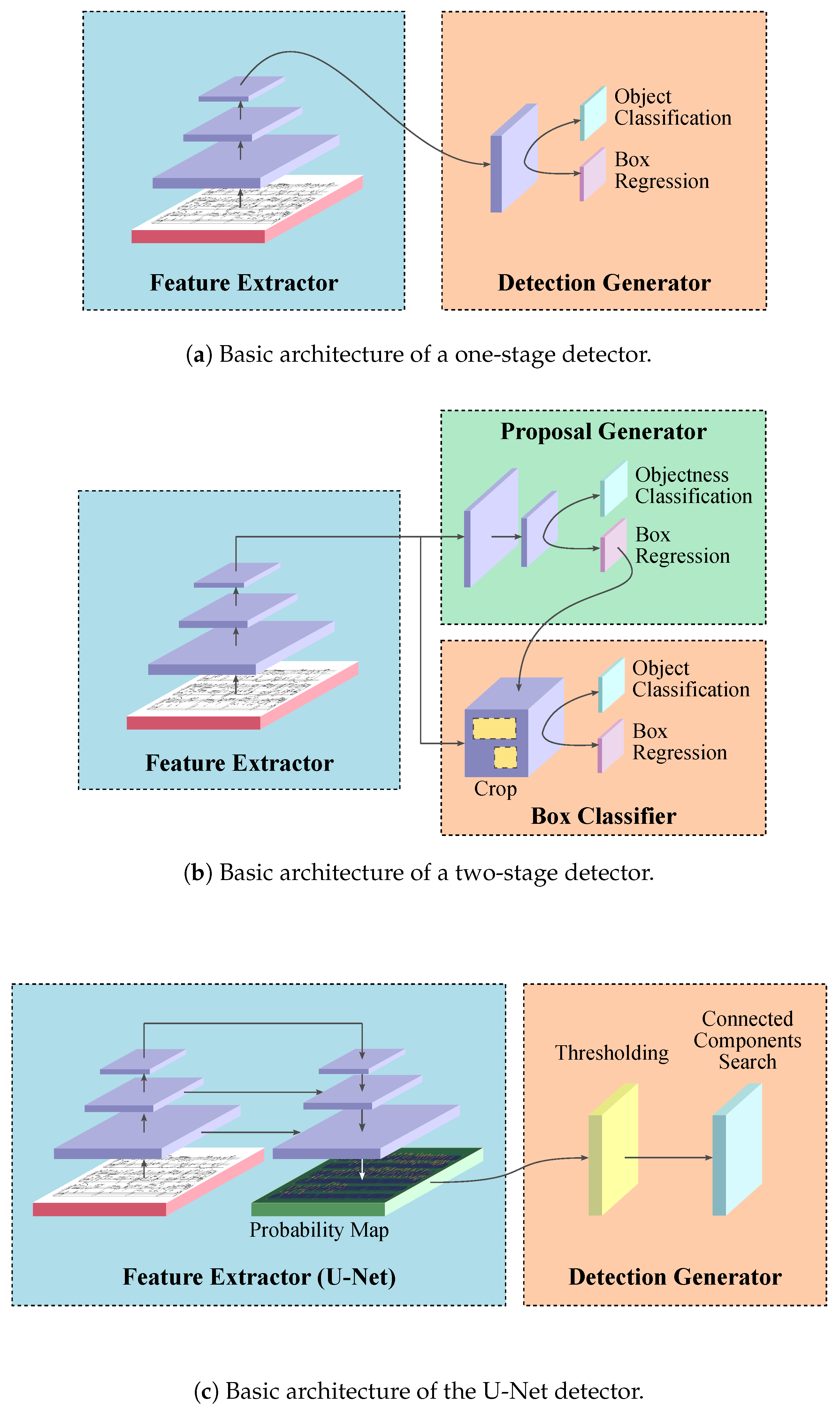
The objective of this work is to provide a good baseline for the music object detection task, and so we consider three neural models of different nature for performing the experiments. While we do want our detectors to be as accurate as possible, we primarily wish to exemplify the different deep learning approaches to object detection. We believe that this is more interesting from the point of view of some reference results, and can help to draw more interesting conclusions. Thus, we use Faster R-CNN as a representative of two-stage detectors, RetinaNet as a representative of one-stage detectors, and U-Nets as a representative of models based on pixel-level segmentation. Figure 1 overviews the general operation of these types of detectors.

4.1.1. Faster R-CNN

Faster Region-based Convolutional Neural Network (Faster R-CNN) [32] is the evolution of the first convolutional network schemes for object detection R-CNN [33] and Fast R-CNN [34]. Faster R-CNN belongs to the class of two-stage detectors, with the first stage generating a sparse set of region proposals that are classified and further refined in the second stage.

While the previous R-CNN schemes used an external mechanism for generating the proposals, such as Selective Search [35] or EdgeBoxes [36], Faster R-CNN attempts to learn the object proposal stage directly from the data employing a region proposal network. The whole process can be carried out efficiently because the convolutional features are shared between both stages, and therefore computing the region proposals does not represent a bottleneck. This also increases the efficiency to train such a network.

The details for training this model followed the recommendations given in the work of Pacha et al. [23]. That is, an Inception-ResNet-V2 [37] is used for the feature extraction stage, initialized with pre-trained weights from ImageNet (as provided by TensorFlow Object Detection API [38]). Input images are rescaled so that the longest edge is no longer than 1000 pixels. A clustering of symbol bounding box shapes is done for each dataset, in order to establish an appropriate set of bounding box shapes to predict, therefore providing appropriate hyperparameters for the object proposal stage.

4.1.2. RetinaNet

The RetinaNet [39] belongs to the family of one-stage detectors that are built on convolutional neural networks. Other prominent representatives are OverFeat [40], Single Shot Detector (SSD) [41] or You Look Only Once (YOLO) [42]. These one-shot detectors create a dense set of proposals along a grid and directly classify and refine those proposals. As opposed to the two-stage detectors, they have to handle a large number of background samples, which potentially can dominate the learning signal.

The RetinaNet [39] is an adaptation of a Residual Network [43] with lateral connections to create features on multiple scales [44]. Small convolutional subnetworks perform classification and bounding box regression on each output layer. RetinaNet was proposed along with the focal loss function, which tries to overcome the hard object-background imbalance issue by dynamically shifting weight to increase the contribution of hard negative examples and decreasing the contribution of easy positives.

The configuration of the network model requires setting several hyperparameters. We specifically checked four different back-ends for feature extraction, namely: ResNet50 [43], MobileNet128 [45], DenseNet121 [46], and a highly simplified version of the DenseNet. Various anchor dimension settings were also examined: the ResNet50 feature extractor performed best in preliminary experiments and was subsequently chosen. The negative overlap threshold was set to 40%, so every box with lower Intersection over Union (IoU) counts as background; similarly, the positive overlap threshold was set to 50%, and every box with a higher IoU is treated as foreground; boxes in between are omitted from the training signal.

4.1.3. U-Net

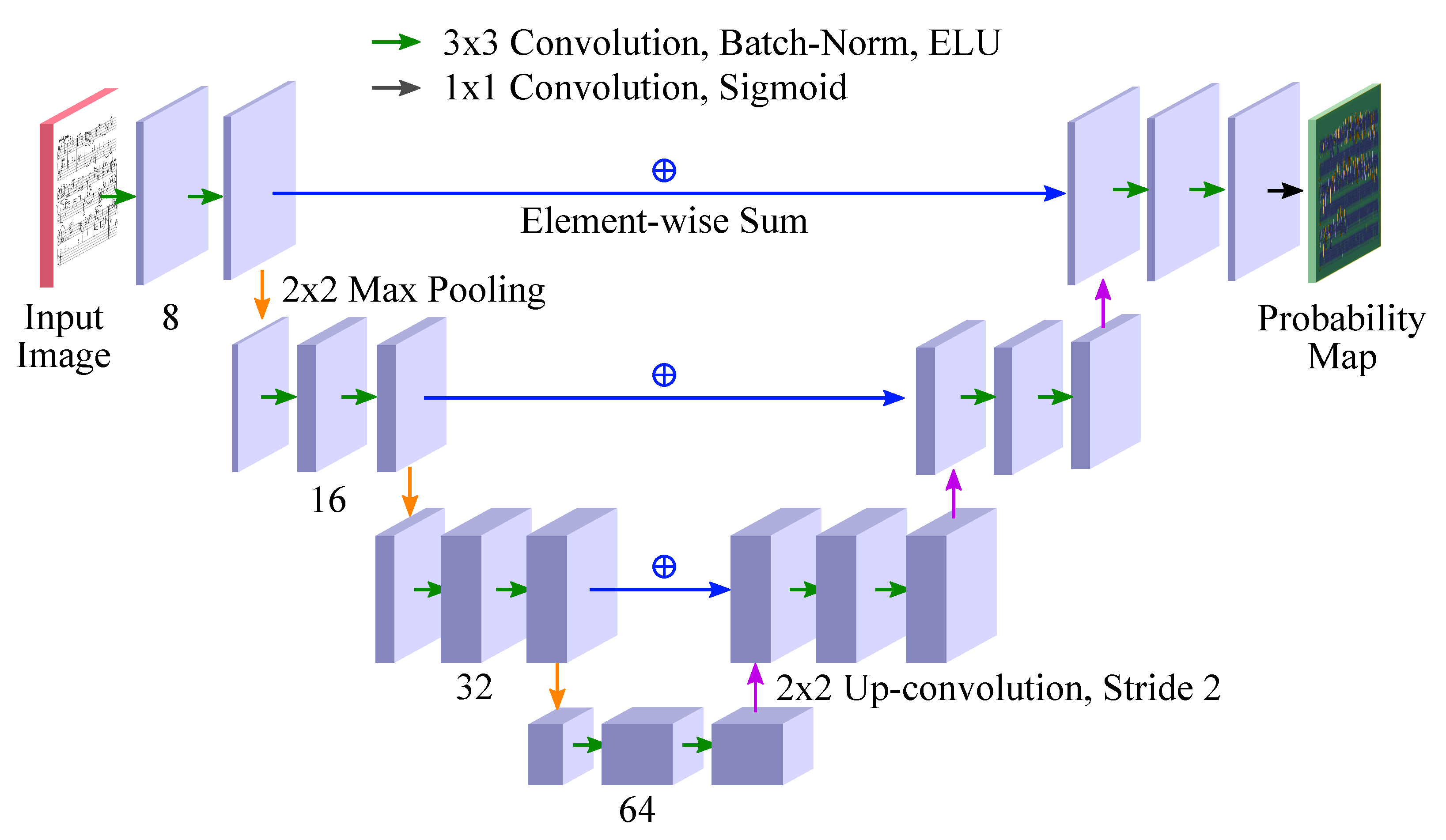
The U-Net [26] is a model for performing semantic segmentation that assigns each pixel of the input image to a certain class. It can be extended to perform object detection, as defined in Section 3. The U-Net architecture combines three key elements: standard 2D convolutions, the “hourglass” architecture inspired by auto-encoders, and residual connections from ResNets [43]. As no other operations than convolutions and element-wise sums of corresponding layers in the “hourglass” are used, the U-Net can in parallel assign a label—or a numerical value, or a probability distribution—to each pixel of an arbitrarily large image. The architecture is depicted in Figure 2.

In order to generate the binary pixel mask training data from the bounding box ground truth, we set all pixels within the bounding boxes of a given symbol class to 1, resulting in rectangular foreground regions for each symbol instance (despite the fact that the symbols themselves are not rectangles).

One drawback of U-Nets is that they were initially designed for semantic segmentation: based on the pixel-wise outputs (such as a probability map), one needs to add a detector stage to actually perform object detection. However, if we thus decide on the detector in advance, we can manipulate the output masks on which we train the behavior of this detector. In the case of music notation, for symbols that may consist of multiple connected components or have complex shapes (the f-clef is an example that combines both), this can be attenuated by training on masks computed from their convex hulls rather than directly from their pixels [25]. Fortunately, as a side effect of using bounding box data in this paper to generate the rectangular pixel-wise masks, we are in essence already getting crude approximations of convex hulls. Note, however, that the bounding box data model thus forces the model to classify background pixels to belong to the symbol, which might otherwise be some way off; this is pronounced especially with beams that are slanted or close to each other.

By not considering the bounding boxes themselves at all during training, U-Nets avoid questions of granularity and the corresponding anchor box hyperparameters, which is a welcome property given the variability of musical symbol shapes—both inter-class and in some cases intra-class. On the other hand, the arbitrary detector step, of course, introduces its own hyperparameters: the masking threshold, and the pixel merging strategy. One can consider the pixel-wise labels as a very fine-grained over-segmentation; the detector then acts as the over-segment merging step. The only architectural hyperparameter one has to set is the size of the receptive field of an output pixel, which is defined implicitly through the number of convolutional and max-pooling layers and their filter sizes; if we fix the size of the network, we can also trade off the receptive field size and resolution by downscaling the images.

Model specifics We follow the architecture of [26] and our U-Nets have four “depth” levels, as depicted in Figure 2. The final layer that produces the probability map uses $1\times 1$ convolutions with just one filter, with a sigmoid activation. (This is an efficient implementation of computing a weighted combination of the convolutional features for each pixel from the second-to-last layer.)

Training setup To go from bounding box ground truth to labels for each pixel, we render the rectangles specified by the bounding box ground truth as foreground. Each image is downscaled with a factor of 0.5. Training is not performed on entire images; instead, in each epoch, we uniformly sample a random $256\times 512$ window from each training image (corresponding to a $512\times 1024$ window from the original image). If this window contains no foreground pixel for the given class, we re-sample up to 5 times; this is a general way of slightly oversampling rare classes.

For each symbol class, one U-Net is trained with exactly the same setup. We use cross-entropy loss, using the Adam optimizer with the default parameters suggested in [47]. Batch size is set to 2. We use a learning rate attenuation schedule: starting from 0.001, if the validation loss does not improve for 50 epochs, we multiply the learning rate by 0.2, a process that is repeated five times. Again, none of these steps are domain specific.

Detection is then performed independently for each symbol class: in this setup, the fact that a pixel is classified as belonging to, e.g., a barline, does not preclude it from also being classified as a stem pixel (note that certain music notation symbols indeed overlap to a great extent, e.g., noteheads and ledger lines). As opposed to [25], we do not experiment with multi-channel outputs, as this is a step that already requires domain-specific knowledge. For the detection stage, we use simple thresholding at 50% and a connected component detector, this time following the setup of [25]. The detector does not output any natural confidence score, so we add a placeholder value of 1 for each detected foreground region.

4.2. Datasets

As we are considering generic object detection methods, we can evaluate all of them across a range of OMR datasets for symbol detection [48]. As a side-effect of this evaluation, we also obtain a notion of the difficulty of these datasets for object detection in general. Each dataset contains a different kind of typography, adding to the breadth of the baselines we establish.

• DeepScores: DeepScores [49] is a very large synthetic dataset of music scores in Common Western Modern Notation (CWMN), consisting of 300,000 images along with their ground-truth annotations for performing symbol classification, image segmentation, and object detection. It is based on a large collection of freely available MusicXML files from MuseScore [50] that were converted into Lilypond files and digitally rendered into images using five different fonts to obtain a higher visual variability. The first version of this dataset only has annotations for a limited vocabulary that is missing essential glyphs, such as stems, beams, barlines, ledger lines or slurs. The second version, which is currently under development, contains these missing annotations and has been made available to us by the original authors. This set contains only 100 pages, but has full annotations for all relevant music symbols.
• MUSCIMA++: MUSCIMA++ [14] is a dataset of handwritten music that has over 90,000 manually annotated handwritten musical symbols in CWMN. The dataset is built on the CVC-MUSCIMA dataset for staff removal [51]. The ground truth is defined as a notation graph: in addition to the individual symbols, their relationships are annotated as well, so that the semantics (pitch, duration, and onset) can be inferred and the full OMR pipeline can be trained on the dataset. However, in this paper, we only focus on symbol detection, equivalent to recovering the vertices of the notation graph.
• Capitan: Capitan consists of 46 fully-annotated pages in Spanish mensural notation from the 16th–18th century. The manuscripts represent sacred music, composed for vocal interpretation. The compositions were written in music books by different copyists of that time. To preserve the integrity of the physical sources, images of the manuscripts were taken with a camera instead of scanning them in a flatbed scanner, leading to suboptimal conditions in some cases. The corpus is based on the dataset used in the work of Pacha and Calvo-Zaragoza [24]. However, the refined version used in this work is focused on obtaining a diplomatic transcript, keeping the information of how symbols were written in the source as intact as possible. That is why there is a higher number of categories, since now symbols that have the same meaning—for example, a minima with the stem pointing up or down—are considered as different categories.

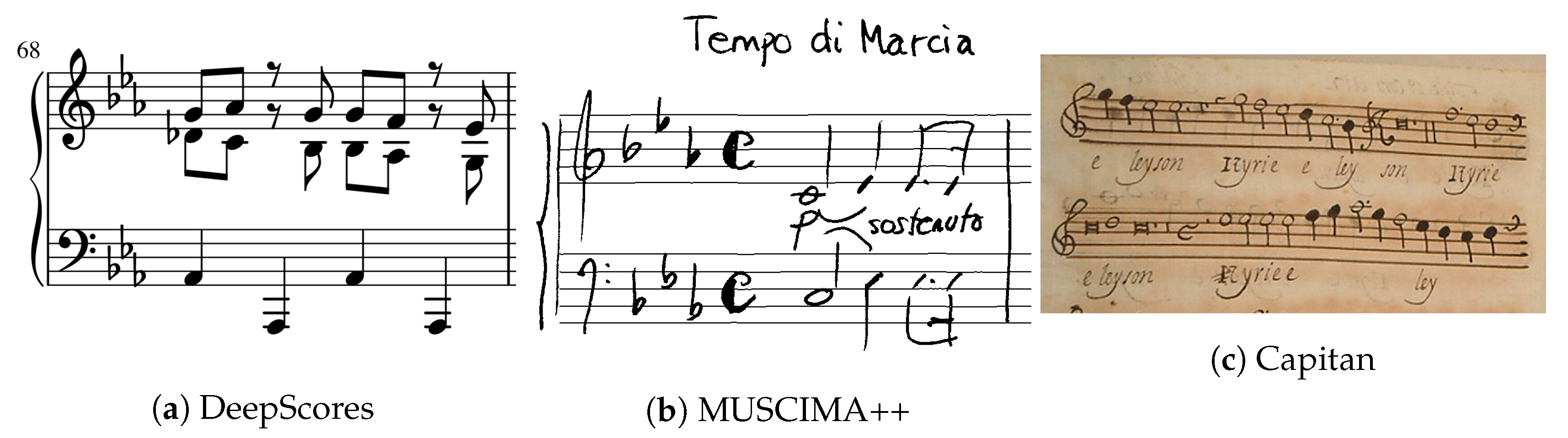
An overview of the corpora considered is given in

Table 1. Overview of the considered datasets.

Dataset	Notation	Engraving	Images	Categories	Scores	Symbols
DeepScores	CWMN	Printed	Binary	39	100	87,703
MUSCIMA++	CWMN	Handwritten	Binary	107	140	91,254
Capitan	Mensural	Handwritten	Color	56	46	11,242

, while we show some patches extracted from their images in Figure 3. As can be observed, the characteristics of the different corpora are quite heterogeneous, which is interesting for drawing generalizable conclusions from our experiments.

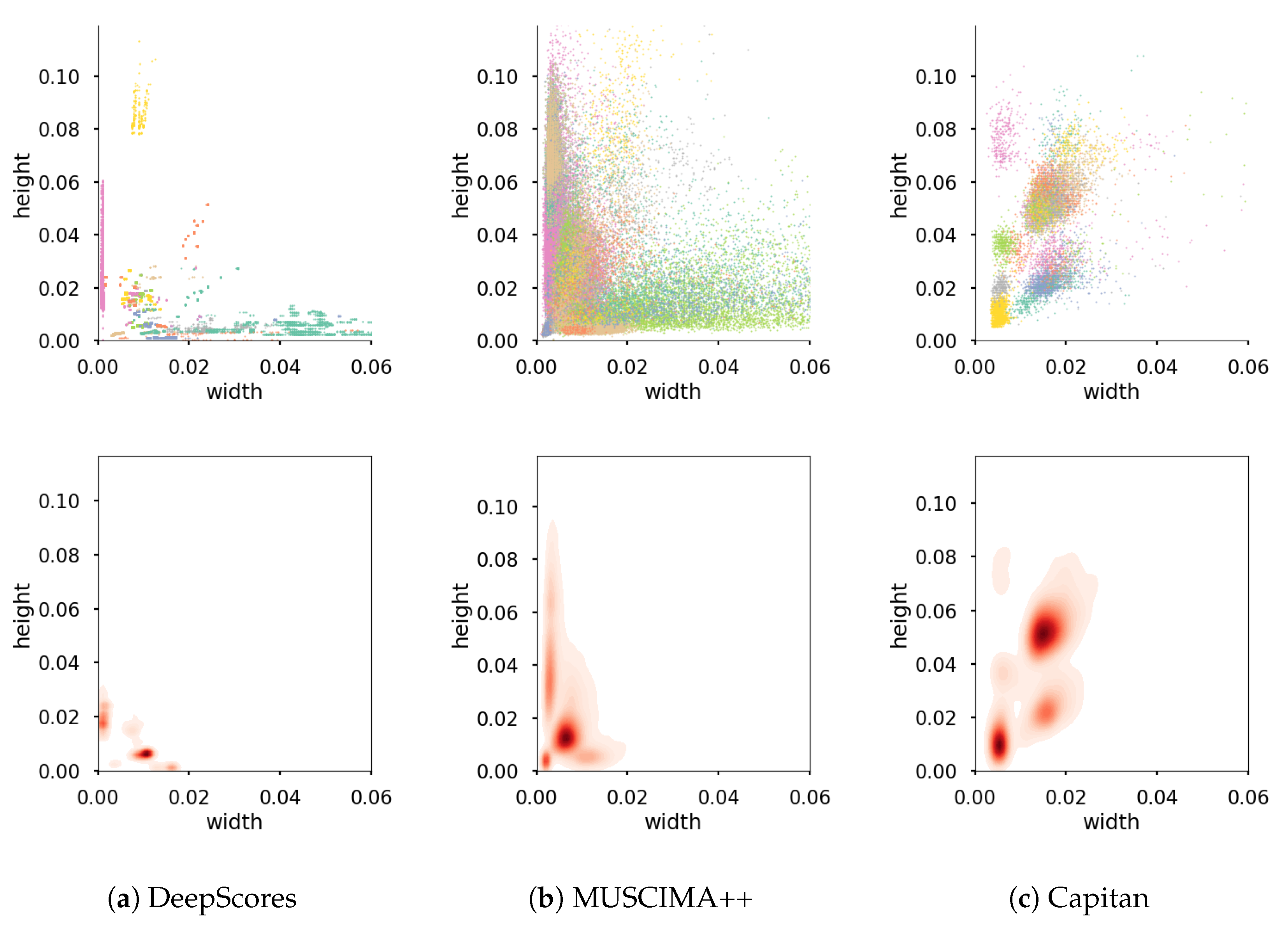
It is important to mention the variability in the aspects of the bounding boxes of the elements within these datasets. This variability appears not only amongst elements of different classes but also, especially in the case of handwritten notation, amongst elements of the same class. To illustrate this scenario, Figure 4 shows the different shapes of the boxes to be recognized in each dataset. The majority of objects in the DeepScores dataset are very tiny. The MUSCIMA++ dataset shows a greater variation in aspect ratios with one dominant cluster, the noteheads. In addition, the Capitan dataset contains a significant number of bigger objects, compared to the other two datasets with distinct clusters.

To evaluate the models in the different corpora, we followed a fixed partitioning scheme for training, validating, and testing. Therefore, the experiments are reproducible, and future results will be directly comparable. Specifically, 60% of the available data is used for training, to learn the values of the neural models; 20% for validation and hyperparameter optimization; and 20% for testing and computing the final evaluation metrics.

4.3. Evaluation

As stated in Section 3, our formulation expects models to provide a set of detection proposals, each of which consists of a bounding box and the recognized class of the object therein. The models are also expected to provide a score of their confidence for each proposal. A bounding box proposal $B_p$ is considered a positive sample if it overlaps with the ground-truth bounding box $B_g$ according to the Intersection over Union (IoU) criterion

$$\frac{\mathrm{area}(B_p\cap B_g)}{\mathrm{area}(B_p\cup B_g)}$$

exceeding a certain threshold ($t_{\mathrm{IoU}}$). If the predicted category matches the actual category of the object, it is considered a true positive (TP), being otherwise a false positive (FP). Additional detections of the same object are considered as false positives as well. Those ground-truth objects for which the model makes no proposal are considered false negatives (FN). From these values, precision (P) and recall (R) metrics can be computed as

$$P=\frac{TP}{TP+FP},R=\frac{TP}{TP+FN}.$$

P measures how reliable detections are (ratio of correct detections), whereas R measures the ability of the model to detect symbols (ratio of detected symbols).

Object detection can be seen as a retrieval task, in which bounding boxes are ordered by their associated scores. Then, P and R can be computed as previously described from the top k predictions. However, different values of P and R are obtained by varying the parameter k. To obtain a single metric encompassing the performance of the model, the average precision (AP) can be computed, which is defined as the area under the precision–recall curve for all possible values of k.

A single AP value is obtained independently for each class, and then the mean AP (mAP) is computed as the average across all classes. Since our problem is highly unbalanced with respect to the number of objects of each class, we also compute the weighted mAP (w-mAP), in which the mean value is weighted according to the frequency of each class. The difference between mAP and w-mAP gives a quick idea of how the evaluated models deal with the rare classes.

When $t_{\mathrm{IoU}}$ is set to 50%, the described evaluation protocol matches the PASCAL Visual Object Classes (VOC) challenge [52]. The accuracy of the localization is especially important for OMR, as objects are often packed densely. Failing to locate them correctly heavily affects the subsequent recognition. To account for this, we average mAP and w-mAP over different values of $t_{\mathrm{IoU}}$, ranging from 50% to 95% by steps of 5%. This evaluation protocol is taken from the COCO challenge [17], and it is expected to provide figures that are more sensitive to precise symbol localization.

5. Results

The aggregate detection performance of the individual models over each of the datasets is reported in

Table 2. Results in terms of mAP (%) and w-mAP (%) with respect to the dataset and object detector model following the COCO evaluation protocol.

	mAP (%)			w-mAP (%)
	DeepScores	MUSCIMA++	Capitan	DeepScores	MUSCIMA++	Capitan
Faster R-CNN	19.6	3.9	15.2	14.4	7.9	23.2
RetinaNet	9.8	7.7	14.5	1.9	4.9	34.9
U-Net	24.8	16.6	17.4	23.3	33.6	26.0

, presenting both mAP and w-mAP as defined for the COCO challenge [17]. These results should serve as the baseline for further music object detection research. Generally, it can be observed that the results are still very far from the optimal. The evaluated models struggle most with the MUSCIMA++ dataset, with the U-Net performing best at around 16% mAP and 33% w-mAP. It might be that the comparison is not entirely fair since the U-Net was specially designed for this dataset. However, U-Net outperforms the rest of the models in the case of DeepScores as well, where it attains around 24% in both mAP and w-mAP, leaving Faster R-CNN and RetinaNet below 20% and 10%, respectively, in both metrics. Concerning the Capitan dataset, all models behave quite similarly, except for the superior performance from RetinaNet regarding the w-mAP metric.

In general, Faster R-CNN performs better than RetinaNet. However, it is especially sensitive to the selection of hyperparameters that regulate the shape and scale of the objects to be detected. The high variability in the bounding box shapes shown in Figure 4 might explain why Faster R-CNN is far from offering the performance it demonstrates for detecting objects in natural images. Compared to previous works that reported 80% mAP for snippets [23] and 76% mAP for full pages [24], a few differences need to be pointed out to understand the large difference between the numbers: the experiments from this work used less training data due to a stricter dataset split, the vocabulary of the Capitan dataset became larger and the final results are computed following the strict COCO evaluation protocol as opposed to reporting the PASCAL VOC metrics [52].

In the case of RetinaNet, an in-depth analysis of its operation reveals that it is not capable of detecting small objects. This explains the noticeable discrepancy between their mAP and w-mAP in DeepScores, where the noteheads—small objects—are the most represented category. Note that Faster R-CNN also exhibits this behavior on the DeepScores dataset, where more frequent symbols are also more problematic for the model than the more rare symbols.

In practical settings, inference speed, and in some situations (re-)training speed, can offset small differences in detection performance. We give a rough comparison when running the experiments on a standard consumer PC, equipped with a GTX 1080 graphics card:

• Faster R-CNN: Training time: 8–12 h; inference time: 20–50 s per image,
• RetinaNet: Training time: 1–2 h; inference time: less than 1 s per image,
• U-Net: Training time: 2–3 h per symbol class; inference time: 40–80 s per image, or about 0.8 s per symbol class.

In this comparison, the RetinaNet has a clear advantage: if one were to find a way to improve its accuracy to an acceptable level, it would be a clear champion for interactive OMR or online recognition settings. U-Nets, on the other hand, are impractical for situations where frequent re-training is needed: unless one has a cluster of graphical processing units (GPUs), training even the minimum 30+ classes that are necessary for pitch and duration inference would take several days.

Qualitative Results

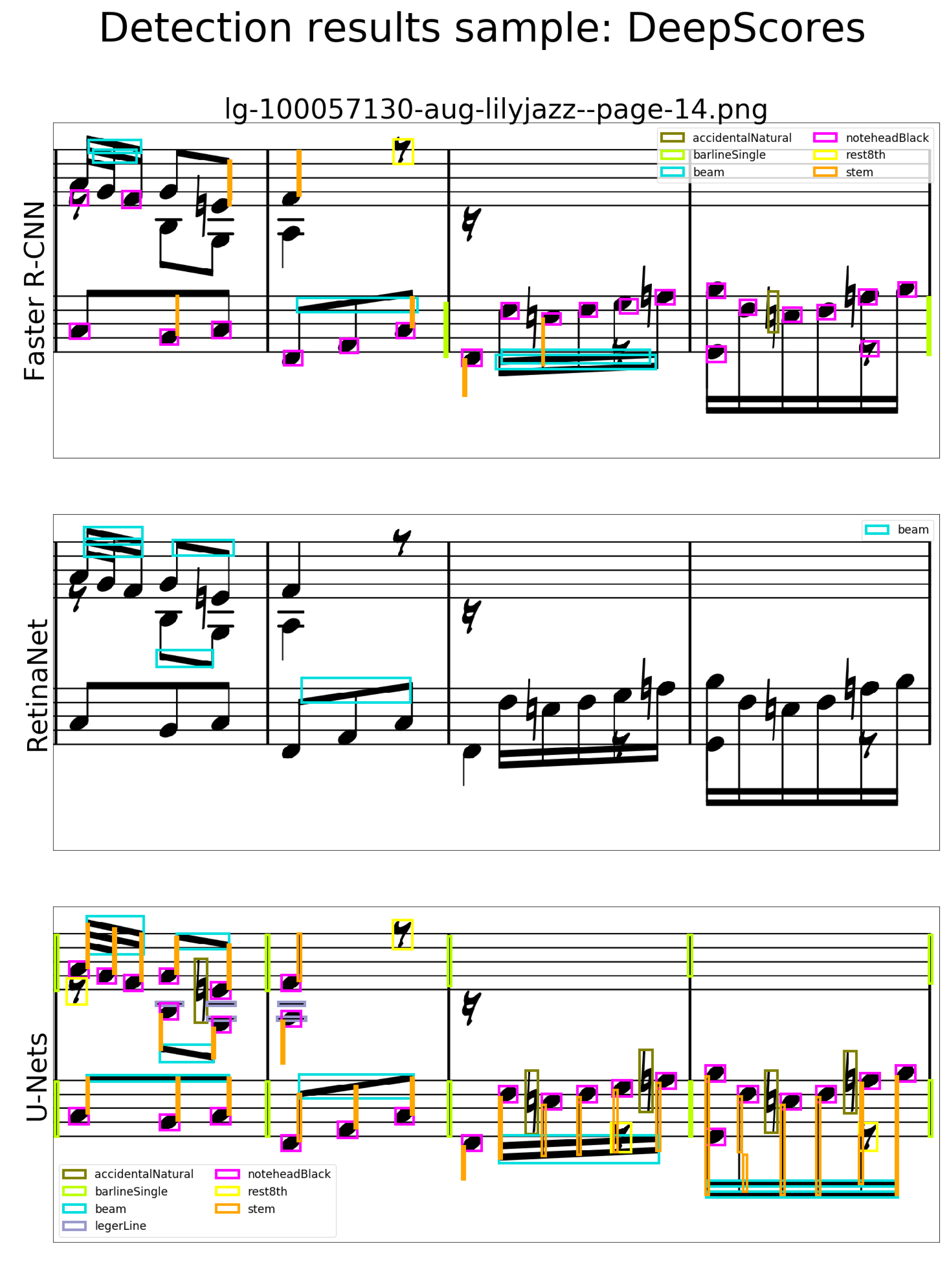
To illustrate the differences in performance, we show samples of detector outputs across the three datasets for some selected classes. Figure 5 shows how the detectors fare with the born-digital printed music of DeepScores. As the rendered symbols have relatively little variability, this sample allows for comparing the strengths and weaknesses of the models’ designs, especially with respect to music notation data.

The Faster R-CNN model (Figure 5 top) has trouble with symbols that are bunched together closely, especially in the upper left corner. This may be due to too few available proposals in a given region. On the other hand, it can distinguish slanted parallel beams (first and third measure). The RetinaNet (Figure 5 middle) is unable to deal with symbols smaller than the beams and does not even find all of them. The U-Nets (Figure 5 bottom) shine in this specific example, perhaps a bit more than the quantitative results suggest: they also recover the heavily overlapping eighth rest in the third and fourth measures. On the other hand, the inherent limitation of the connected component detector causes beams with overlapping bounding boxes to get lumped together. If one were to choose an image with dense chords, noteheads within a chord would also invariably get merged into one.

Detection performance on the MUSCIMA++ dataset (Figure 6) displays a similar pattern. The RetinaNet again cannot detect anything but the large objects; Faster R-CNN again seems to run out of proposals in cluttered regions, or perhaps proposals get inadvertently merged into one due to insufficient feature map resolution. U-Nets are lucky in this image: the descending thirds in the first measure are just far enough from each other so that they get detected separately; if they were as close to each other as the bottom two noteheads on the third and fourth beat of the second measure of the sample, they would get merged into one. Beams, even though their bounding boxes do not necessarily overlap (bottom staff, second measure), again get merged, and there are false positive beams in hairpins.

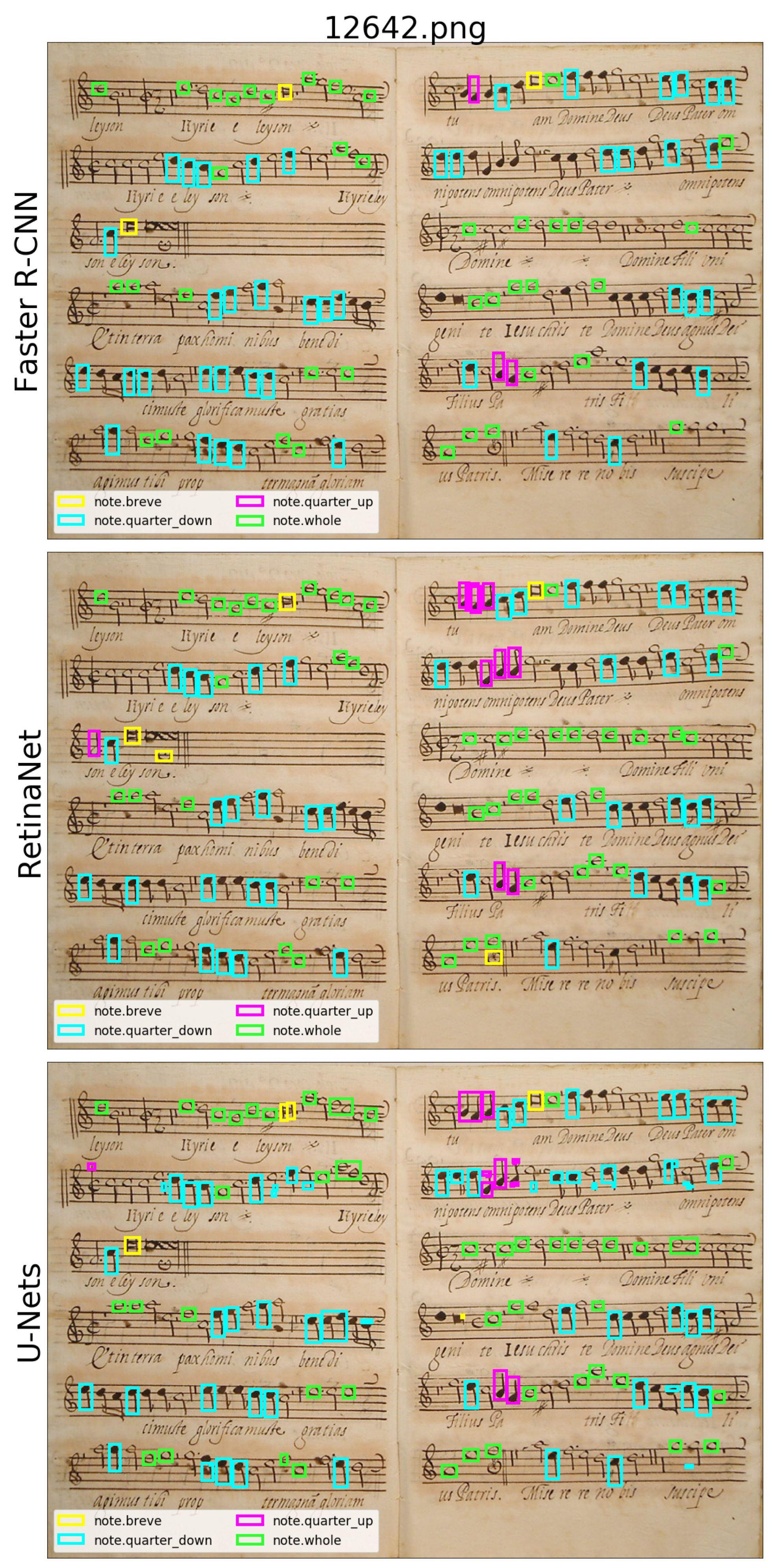
On the Capitan dataset, the situation changes, as illustrated in Figure 7. We hypothesize that the main driver for this difference is the change in symbol class definition: instead of using notation primitives such as noteheads or stems, the Capitan dataset uses composite symbols such as note.quarter-up, note.beamedLeft1. This discrepancy in defining music notation objects has persisted throughout the literature on music object detection [19].

This presents a problem for the U-Nets: the most prominent feature of a note, whether facing down or up, is the notehead. As the symbols are processed independently, there is a risk that noteheads will be detected as instances of all applicable objects according to the notehead type. If one looks at the U-Nets’ output (Figure 7 bottom), e.g., the middle of the second staff on the second page, eighth notes get classified as quarter notes, and half-note stems fool the quarter-note detector into false positives. In addition, as the symbols get larger, the U-Net runs into one of its inherent risks concerning the connected components detector: symbol fragmentation. As the pixels of symbols that are easily classified tend to be on their extremes, the system may become less certain in their centers, and the symbol falls apart after thresholding the U-Net output probability map. We have observed this behavior on barlines and long stems on the MUSCIMA++ dataset as well. This breakup produces many false positives (in Figure 7, especially for quarter notes).

On the other hand, while Faster R-CNN still struggles—although to a much smaller extent—with false negatives, RetinaNet does not face too small symbols anymore, and learns well: when symbol class frequencies are used to weight the result, it outperforms both contenders by a large margin. It falls into none of the U-Nets’ traps.

What can we say regarding the datasets?

For DeepScores, our results seem to confirm the intentions of the dataset authors: the main difficulty of the dataset is the large number of tiny objects [49]. While Faster R-CNN does outperform the same baseline architecture of [49] (which, according to the authors, does not detect anything at all), it does still encounter the limitations that they expected of this class of models. The single-shot RetinaNet detector runs into even worse trouble (and thus the authors of [49] were probably right to not use single-shot detection at all).

The Capitan dataset seems to present a more straightforward object detection challenge. The close relationship of the composite object classes does not seem to be a problem for standard detectors; semantic segmentation, however, struggles.

From the perspective of music object detection, the MUSCIMA++ dataset has turned out to be essentially a more difficult version of DeepScores: the ground truth is defined at the level of notation primitives, the music contained in the datasets has similar complexity, but MUSCIMA++ is handwritten, which makes the shapes more variable, and topological features such as corners less reliable.

6. Conclusions

In this work, we establish a baseline for detecting music notation objects with deep learning models for generic object detection. Experiments were performed over three diverse major OMR datasets: the synthesized DeepScores dataset of born-digital modern notation, the MUSCIMA++ dataset of handwritten modern notation with varying degrees of writing quality, and the Capitan dataset that contains mensural notation which is also handwritten, but of consistently high quality. Three types of neural models have been evaluated, namely the two-stage Faster R-CNN detector, the one-stage RetinaNet detector, and the U-Net detection mechanism that combines flexible semantic segmentation with a connected component detector. The choice of experimental setup and evaluation in this paper can serve as a basis for further music object detection experiments that will, therefore, be directly comparable to these baselines and will enable drawing conclusions and model design recommendations from these direct comparisons.

Based on the quantitative and qualitative results in this paper, can we already formulate tentative practical recommendations for choosing a certain detection approach over another? We are well aware that three datasets may not be enough to draw such general conclusions; however, it is the most comprehensive experimentation that the current state of the OMR concerning available data allows. The suggestions should, therefore, be treated as tentative suggestions for further targeted investigations rather than fully-fledged conclusions.

U-Nets, except for merging nearby symbols of the same class, do not seem to have a problem with the recall. Because they process symbol classes independently and do not reduce the output features resolution, they cannot run into the same (hypothesized) problems as Faster R-CNN, which has a limited number of region proposals for any single region of the image that the symbols in effect compete for. The number of available proposals depends on a hyperparameter setting that might be difficult to set appropriately for areas densely populated of ground truth objects. Furthermore, the proposal merging step (such as non-maximum suppression) may also lead to false negatives in cluttered environments. None of these disadvantages concern the U-Nets.

On the other hand, while these properties are ideal for very cluttered data where symbol classes are set to notation primitives, the design drawbacks of U-Nets do appear when the symbol vocabulary consists of composite symbols; conversely, this is where the cluttering that presumably hinders the bounding box-based models ceases to be an important factor, and the relative strength of these models—the ability to consider a particular region as a whole—becomes more relevant because composite symbols share visual elements that correspond to the primitives. The choice of a musical symbol detection model, therefore, seems to be based on the way the detection ground truth is defined.

Now that a deep learning baseline for music object detection has been established, where can subsequent research be heading?

First, one can use the first insights gained from comparing the models over various datasets to improve the music object detectors themselves. The weak point of U-Nets seems to be settings with composite objects; experiments with composites built from MUSCIMA++ primitives by leveraging their syntactic relationships would be a logical step to investigate this. In order for U-Nets to improve on datasets with composite symbols (which are cheaper to annotate, as they generally contain fewer symbol instances, and therefore more likely to be encountered during various music digitization efforts), a combination of the pixel-wise approach, which deals very well with highly cluttered areas or occlusion, and combined properties of the resulting pixel groups can be a viable avenue, while also perhaps alleviating the problem of parallel beams. In [28], a YOLOv3-like approach has been used to detect noteheads with joint pixel classification and bounding box regression. A post-filtering step then significantly improved precision, which is a much bigger problem for U-Nets than recall. The Deep Watershed Detector used by [27] exhibits a similar combination.

For improving the Faster R-CNN results on music notation data, we would need a better understanding of the relationship between anchor hyperparameters and expected symbol density. The inability of the RetinaNet to detect small symbols is disappointing and merits further investigation, as it persisted regardless of various anchor hyperparameter settings. An idea to test the hypothesis of some minimum detectable absolute symbol size would be to upscale the image until the objects of interest reach sufficient size, and run detection on windows of the upscaled image that fit into GPU memory. The speed of this model both in training and inference would make it an attractive choice for interactive OMR, which is now probably the most viable approach towards building OMR systems that can best support creating digital editions of music, such as the Ceres system [53] or the Pixel.js editor [54].

More can also be done in terms of evaluation to make the baseline more informative regarding the outputs expected from OMR downstream. While music object detection is a critical step in OMR pipelines, it is not the final step; for evaluating a detector as part of an OMR system, one should be able to attribute downstream errors, e.g., in pitch or duration inference, to detection errors or uncertainties. For instance, Ref. [25] uses several ways of evaluating MIDI inferred on top of the object detection results, using a baseline reconstruction model. Furthermore, the graph model of MUSCIMA++ offers hope that the edges can serve as “conduits” from higher-level errors to their lower-level causes, but, so far, we are not aware of any method that would allow combining such structured gradient flows with the object detection architectures.

Then, there are exciting challenges of transfer learning. Modern notation follows the same underlying rules, regardless of whether it is printed or handwritten: can one leverage a printed music dataset to train for handwritten object detection? At least between DeepScores and MUSCIMA++, many symbol classes can be directly mapped onto each other—experiments in this direction should be possible. In this context, the effect of image deformations and other, perhaps more realistic data augmentation can be explored.

Finally, while it is obvious that merely detecting the musical elements in score images does not represent a complete OMR system, we believe that addressing music object detection in a generic machine learning manner brings a series of changes that are quite interesting for the development of the OMR field. Except for the few attempts at end-to-end OMR that are so far limited to monophonic output [7,8,55], all OMR systems are explicitly detecting music objects at some point in their recognition pipeline. Generic deep learning approaches may have the potential to decouple object detection from actual knowledge of music notation itself—nevertheless, users now need to be aware of how these systems learn and design them accordingly. The proposed general machine learning approach can then be used by all of them, regardless of the musical notation system (except for hyperparameter tuning and cookbook-style model choice recommendations), as opposed to approaches that exploit specific characteristics of how the music notation system works to build segmentation heuristics. Then, as the music object detection stage is done, image processing can in principle be forgotten: the only remaining link to the original image is the bounding box and potentially pixel mask features associated with the detected objects. The remaining stages—notation reconstruction and exporting an output representation—then, in turn, do not require computer vision knowledge (while now requiring, of course, some understanding of how music notation stores content). On the other hand, one can utilize the syntactic regularities of music notation to improve the object detection stage (and perhaps perform detection and relational understanding jointly). Incorporating the graph structure, and further prior knowledge about the properties of music notation (such as expected voice leading), into a differentiable loss function that can be optimized by the neural network learning process, represents an interesting avenue for future research. Both approaches, therefore, open up the possibility for experts from different areas to establish a synergy that pushes the development of the OMR field from both perspectives.