Author Contributions
Conceptualization, W.Z.; Data curation, H.T.; Funding acquisition, W.Z. and T.W.; Investigation, W.Z., H.T., and C.Z.; Methodology, W.Z.; Project administration, W.Z. and T.W.; Supervision, W.Z. and T.W.; Visualization, H.T. and C.Z.; Writing—original draft, W.Z.
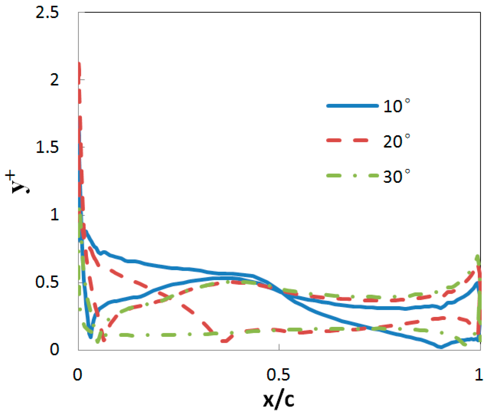
Figure 1.
The wall y+ distribution around the airfoil at angles of attack of 10°, 20° and 30° (Re = 1 × 10⁶).
Figure 1.
The wall y+ distribution around the airfoil at angles of attack of 10°, 20° and 30° (Re = 1 × 10⁶).
Figure 2.
Computational domain for the rotor simulation (“D” is the rotor diameter).
Figure 2.
Computational domain for the rotor simulation (“D” is the rotor diameter).
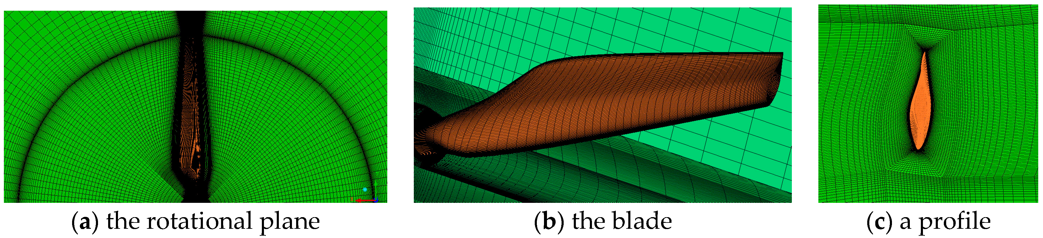
Figure 3.
Demonstration of the mesh adopted for the rotor simulation. (a) The rotational plane; (b) the blade; (c) a profile.
Figure 3.
Demonstration of the mesh adopted for the rotor simulation. (a) The rotational plane; (b) the blade; (c) a profile.
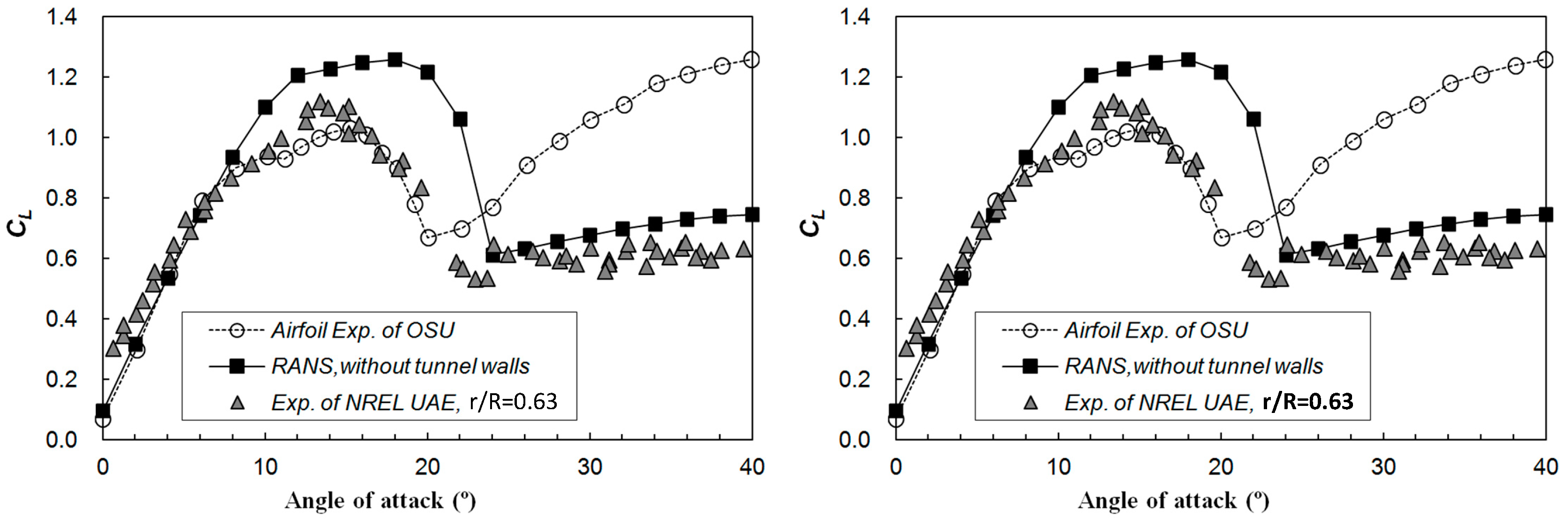
Figure 4.
The computational and experimental lift coefficients of the S809 airfoil.
Figure 4.
The computational and experimental lift coefficients of the S809 airfoil.
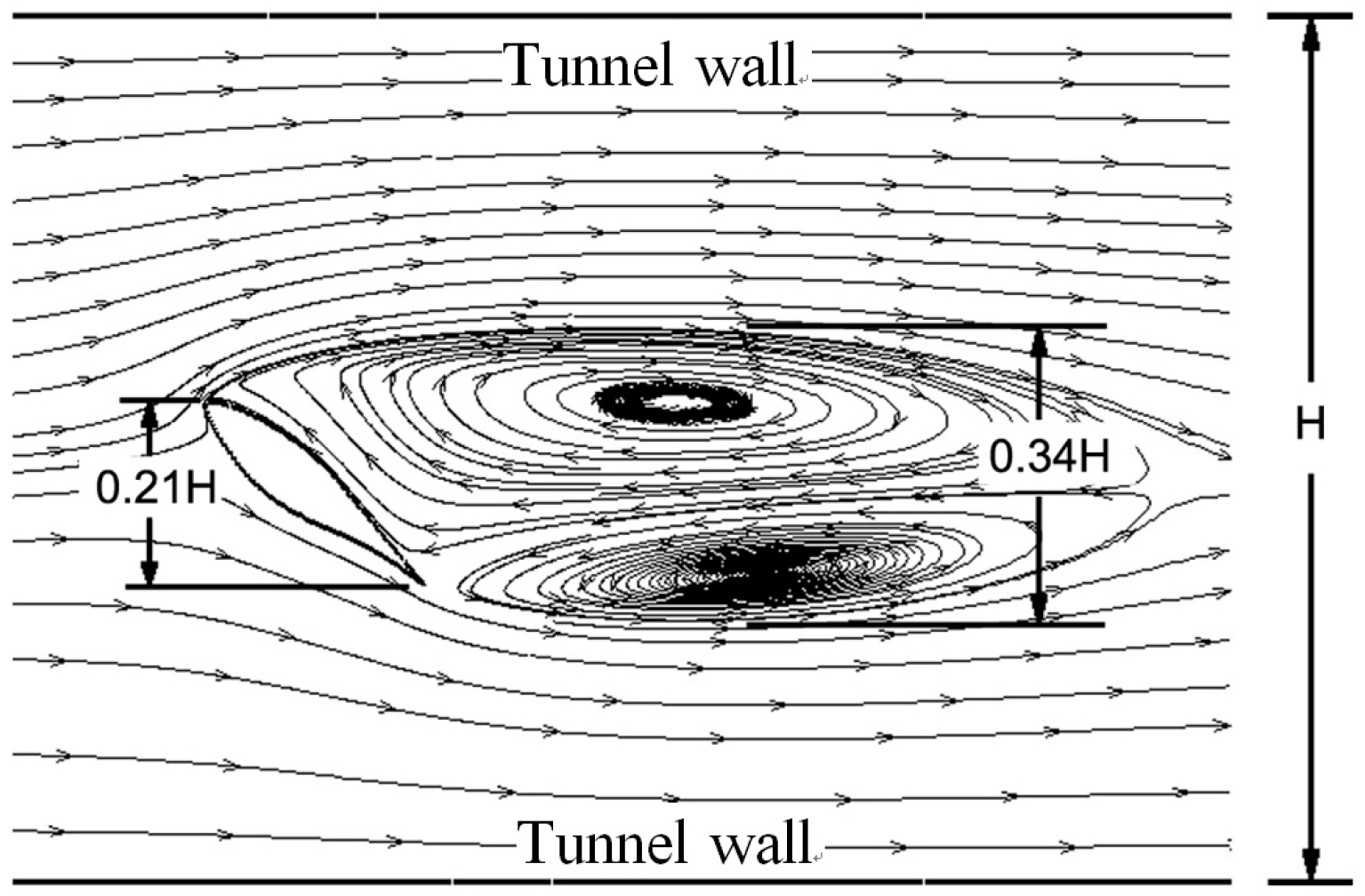
Figure 5.
The simulated flow field of the S809 airfoil in the test section of the wind tunnel of OSU. (AoA = 40°, H = 1.4 m).
Figure 5.
The simulated flow field of the S809 airfoil in the test section of the wind tunnel of OSU. (AoA = 40°, H = 1.4 m).
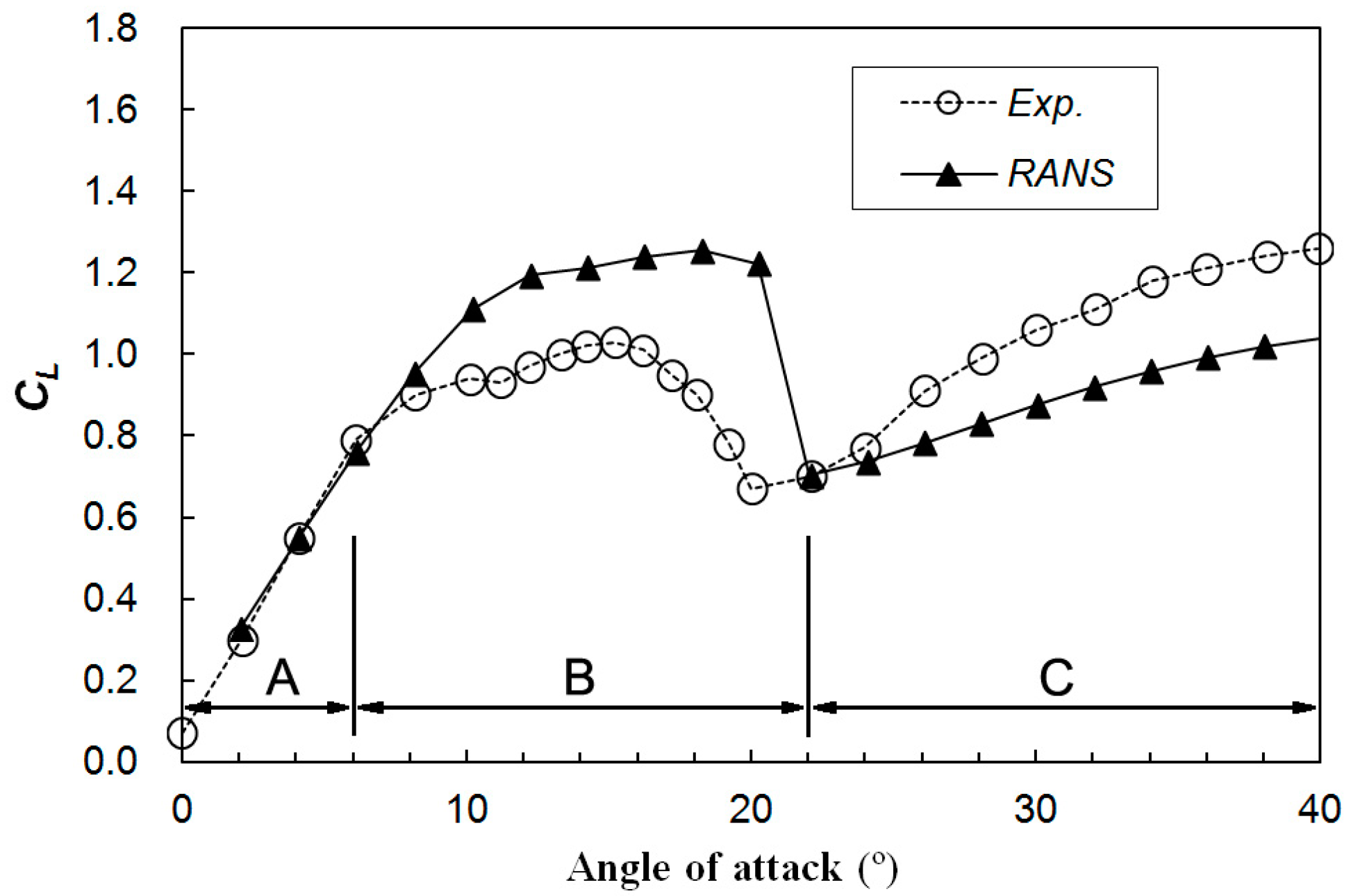
Figure 6.
The lift coefficient from the airfoil simulation with tunnel walls, with a comparison to the measured data of the OSU experiment.
Figure 6.
The lift coefficient from the airfoil simulation with tunnel walls, with a comparison to the measured data of the OSU experiment.
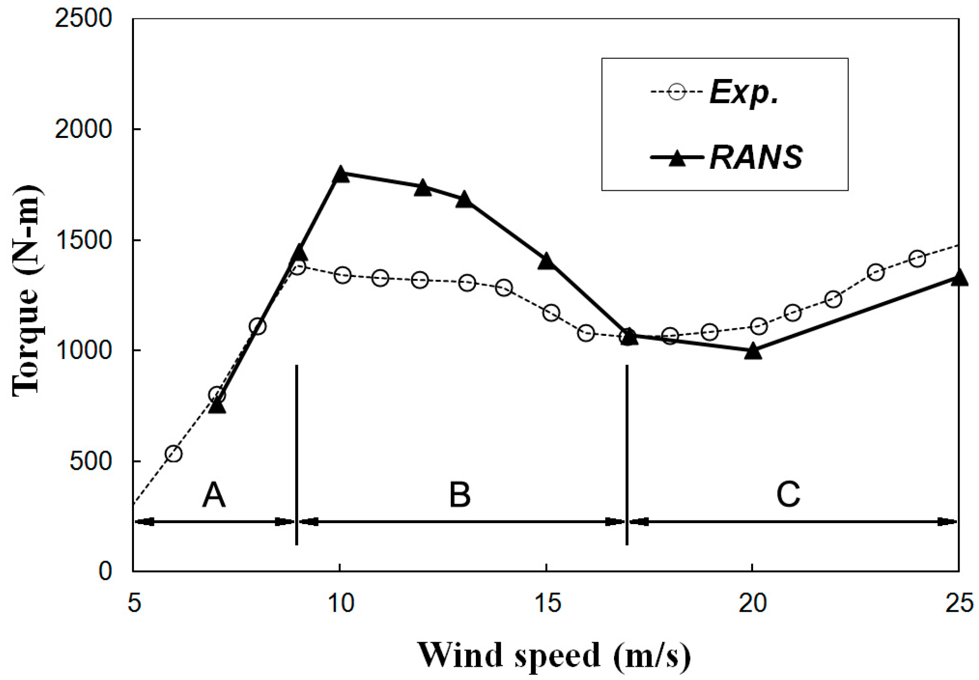
Figure 7.
The predicted torque of the NREL Phase VI rotor, with a comparison to the measured data.
Figure 7.
The predicted torque of the NREL Phase VI rotor, with a comparison to the measured data.
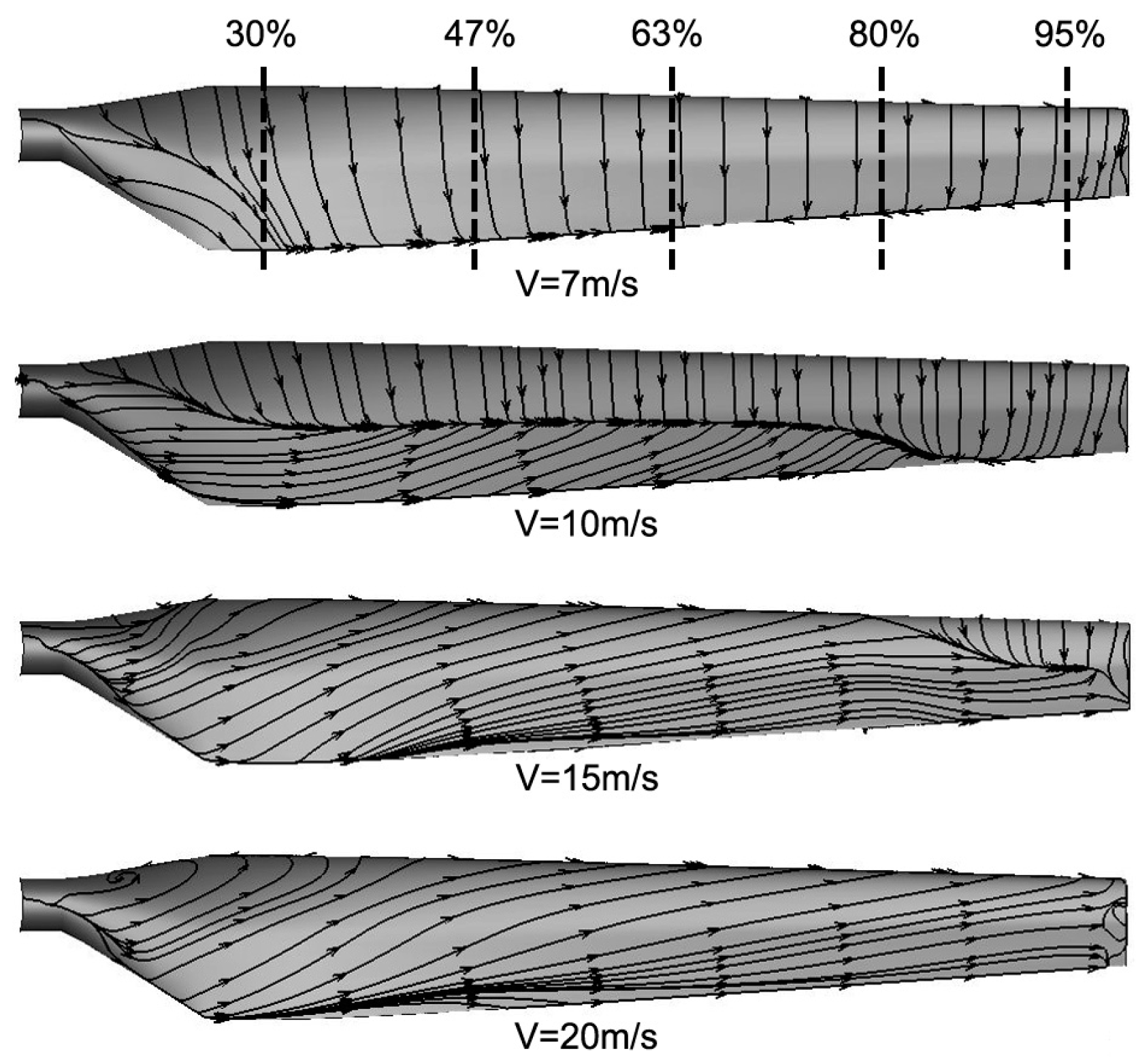
Figure 8.
The simulated limiting streamlines on the suction side of the NREL Phase VI blade at various wind speeds.
Figure 8.
The simulated limiting streamlines on the suction side of the NREL Phase VI blade at various wind speeds.
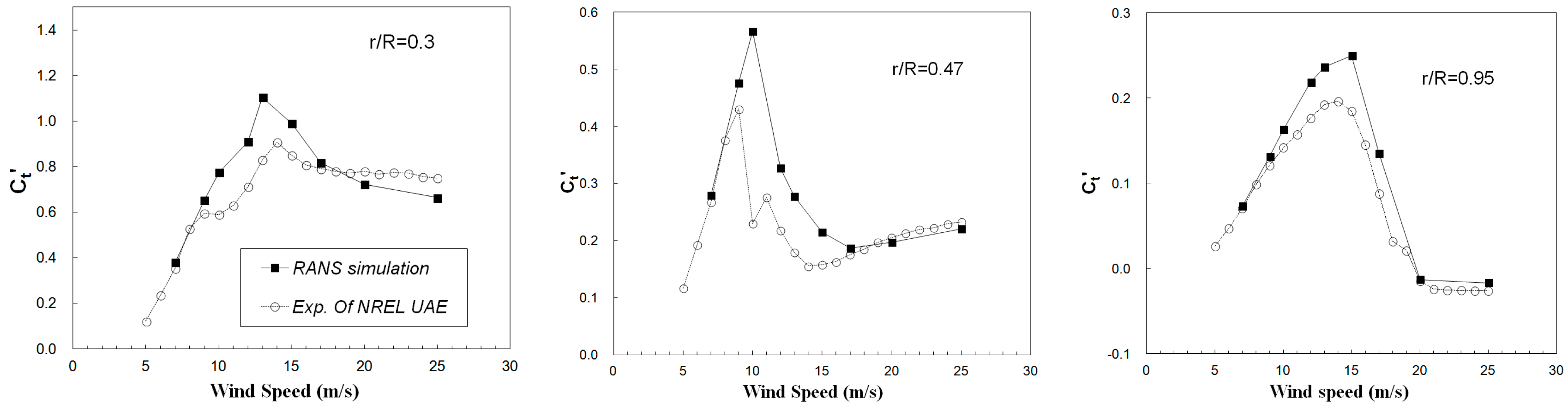
Figure 9.
The predicted Ct′ versus wind speed at three typical blade sections, with a comparison to the measured data of the NREL Phase VI experiment.
Figure 9.
The predicted Ct′ versus wind speed at three typical blade sections, with a comparison to the measured data of the NREL Phase VI experiment.
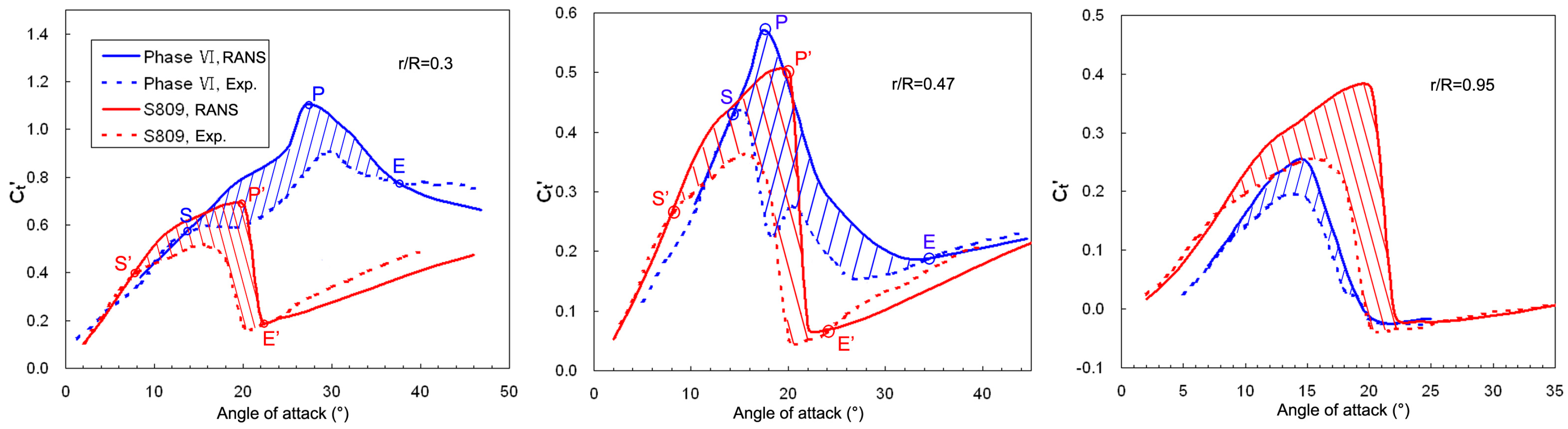
Figure 10.
The Ct′ versus AoA at different blade sections, with a comparison to the corresponding curves of the S809 airfoil.
Figure 10.
The Ct′ versus AoA at different blade sections, with a comparison to the corresponding curves of the S809 airfoil.
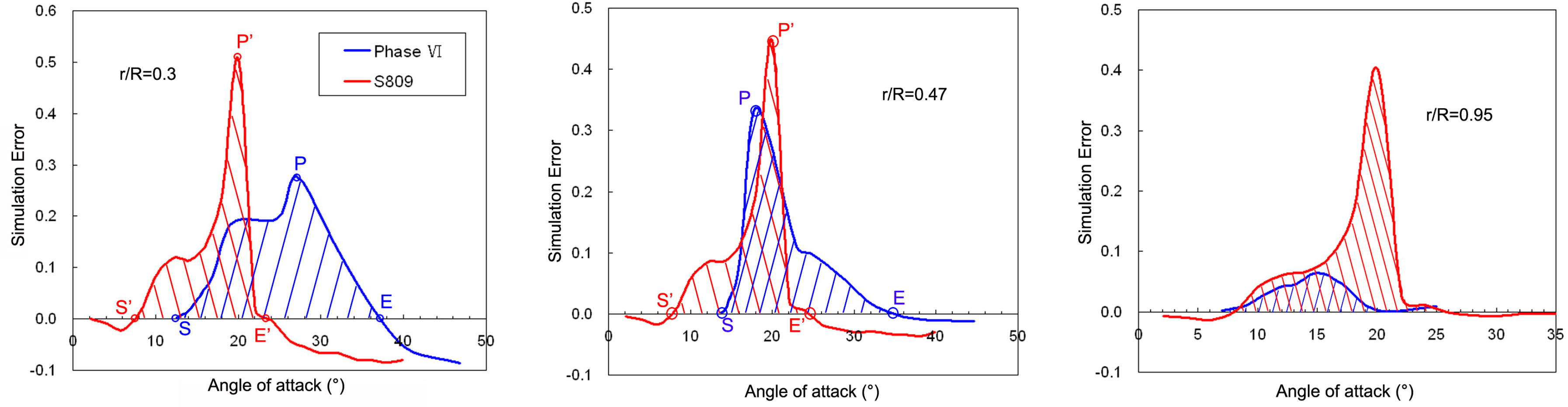
Figure 11.
The magnitude of the simulation error at different blade sections, with a comparison to the corresponding curves of the S809 airfoil.
Figure 11.
The magnitude of the simulation error at different blade sections, with a comparison to the corresponding curves of the S809 airfoil.
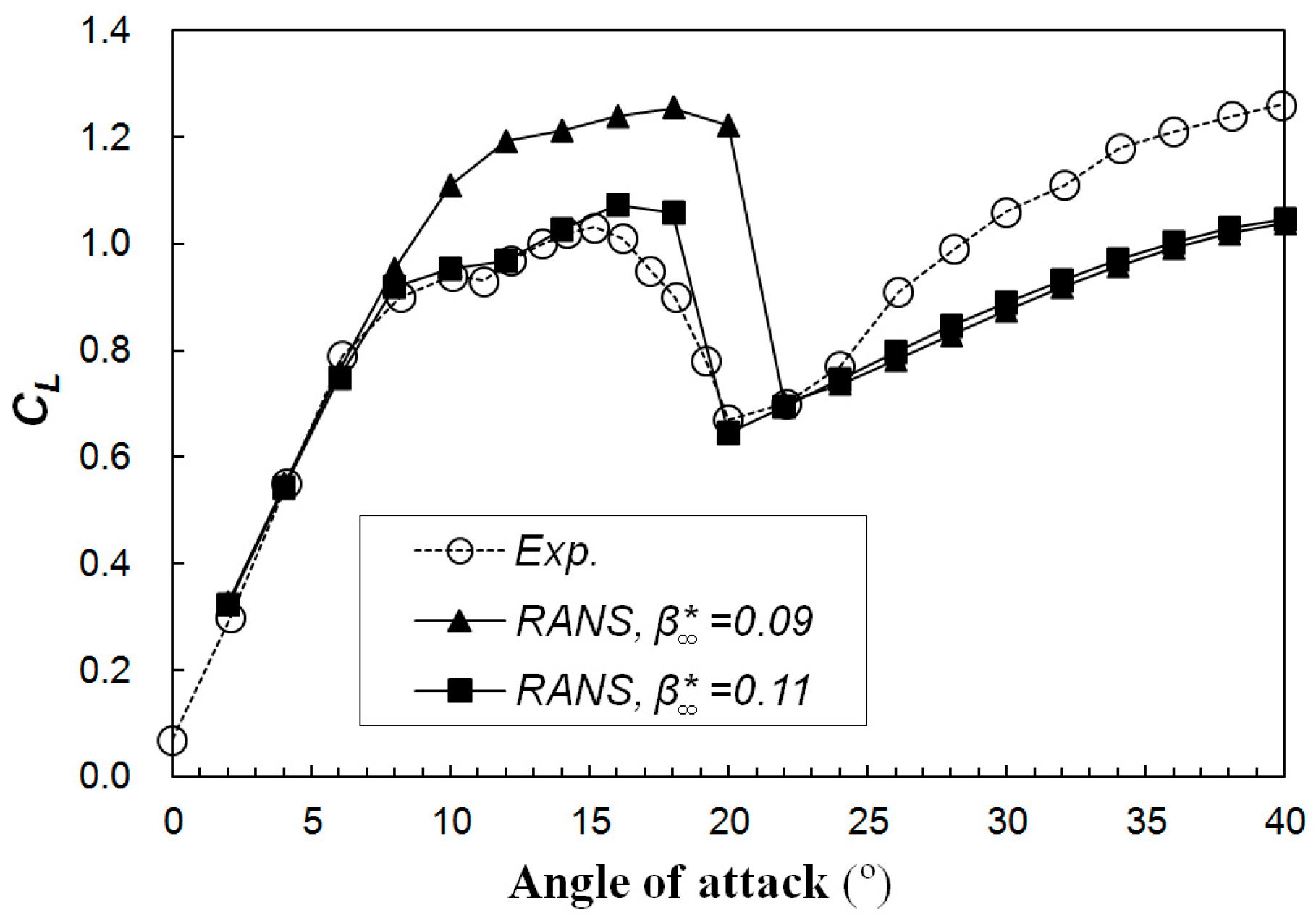
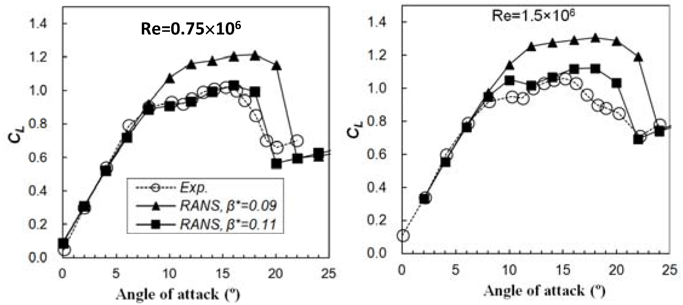
Figure 12.
The simulation results of lift coefficient for different values of compared to experimental data. (Re = 1 × 10⁶).
Figure 12.
The simulation results of lift coefficient for different values of compared to experimental data. (Re = 1 × 10⁶).
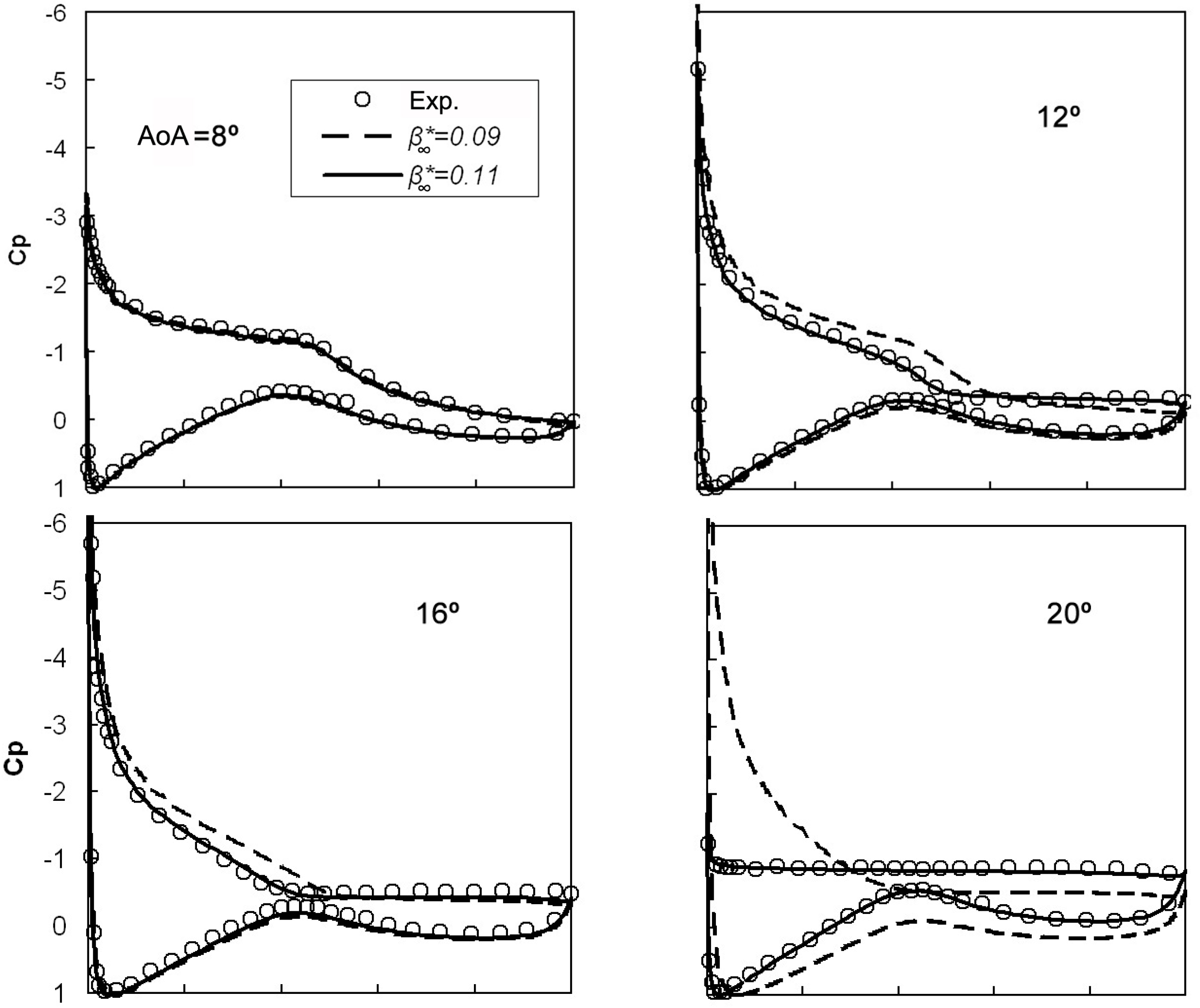
Figure 13.
The predicted pressure distributions for different values of , with a comparison to experimental data (Re = 1 × 10⁶).
Figure 13.
The predicted pressure distributions for different values of , with a comparison to experimental data (Re = 1 × 10⁶).
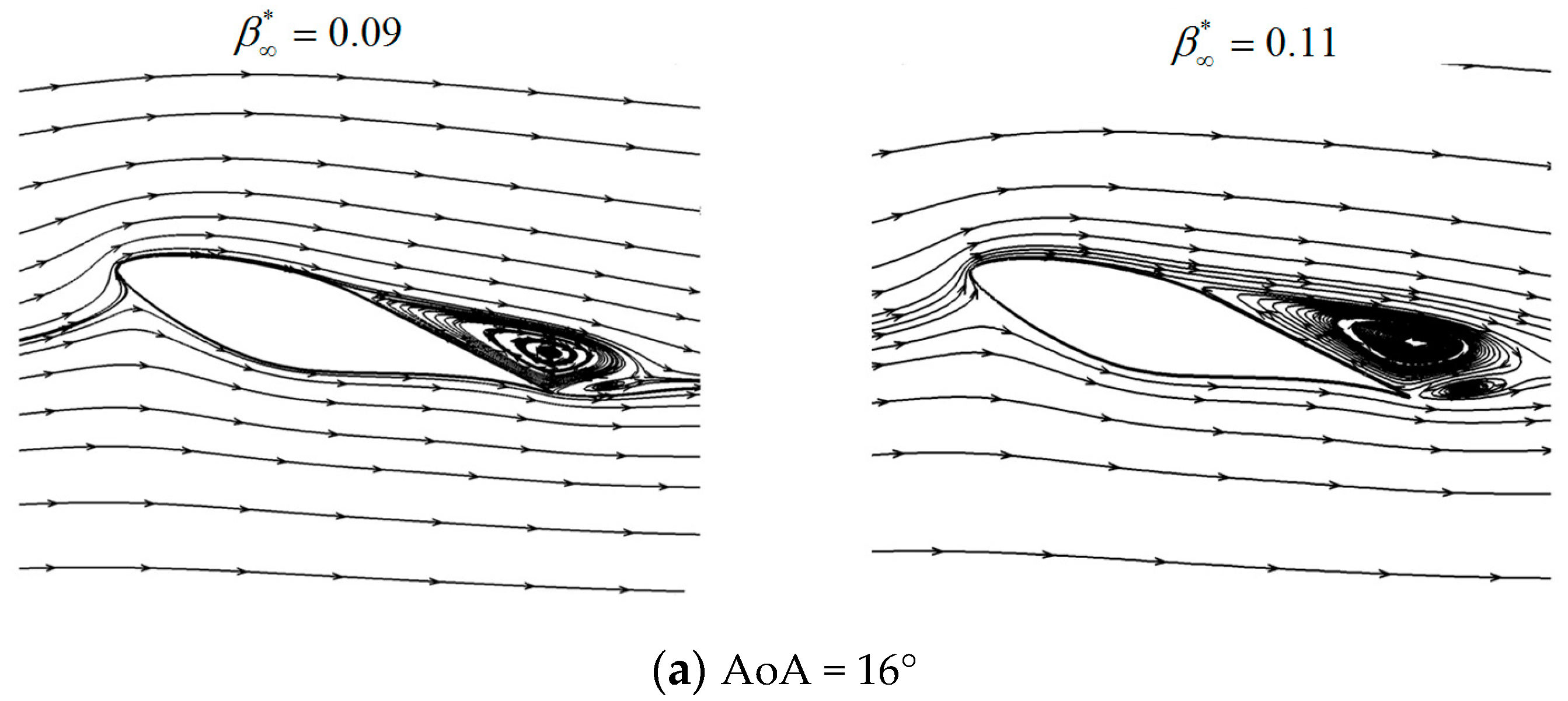
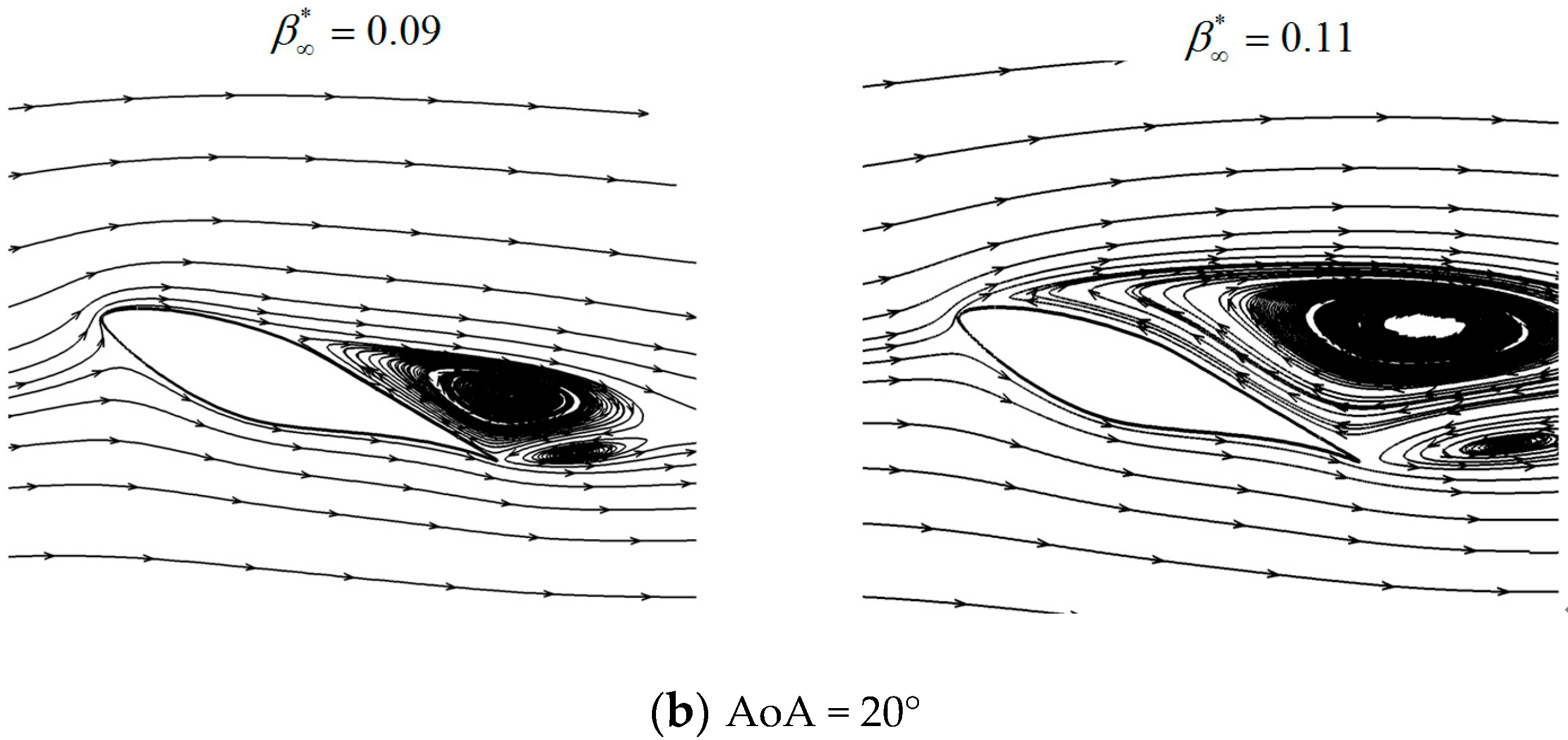
Figure 14.
The simulated streamlines around the airfoil for different values of (Re = 1 × 10⁶).
Figure 14.
The simulated streamlines around the airfoil for different values of (Re = 1 × 10⁶).
Figure 15.
The simulation results of lift coefficient at different Reynolds numbers compared to experimental data.
Figure 15.
The simulation results of lift coefficient at different Reynolds numbers compared to experimental data.
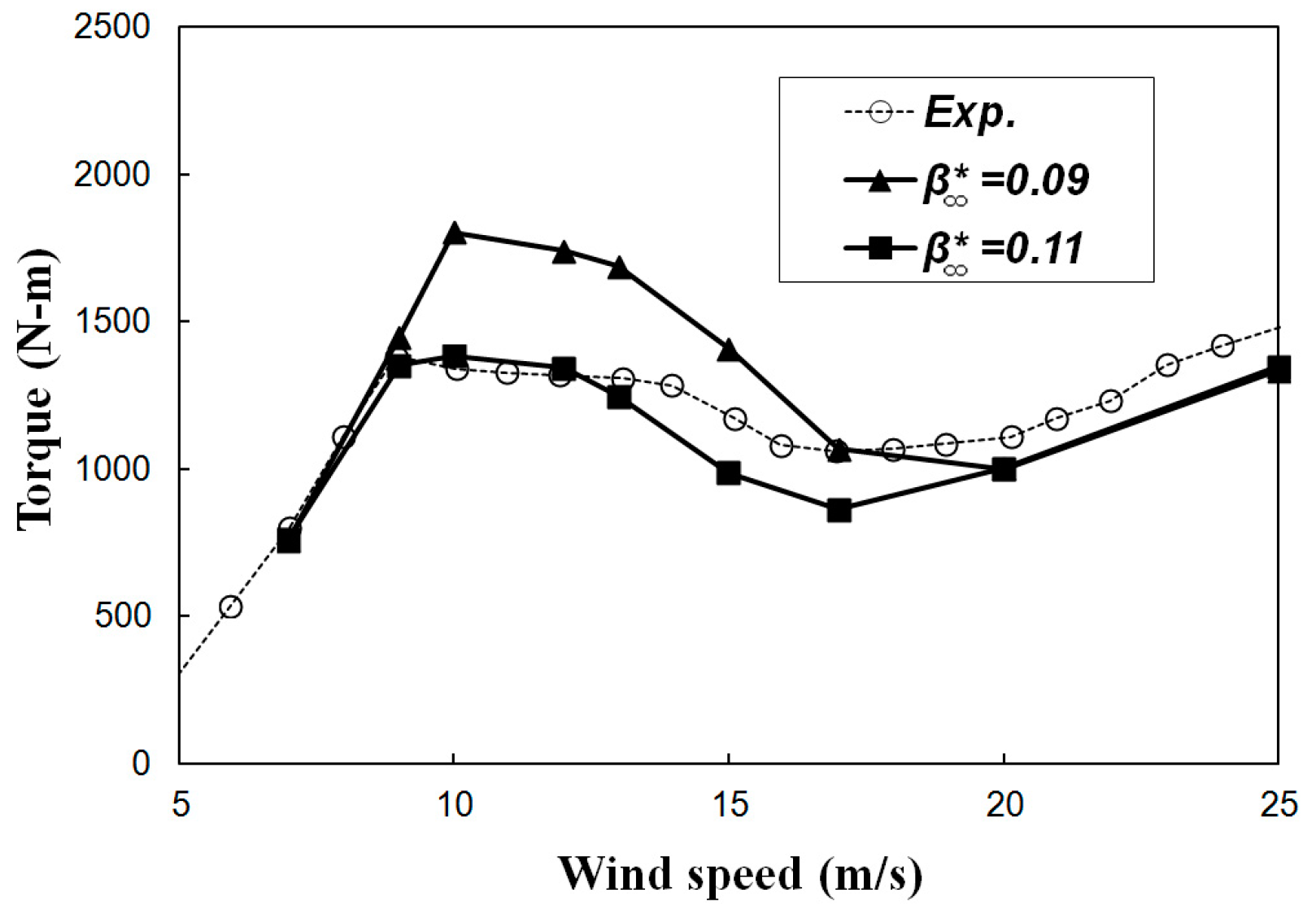
Figure 16.
The predicted rotor torque for different values of compared to the measured data of the NREL Phase VI experiment.
Figure 16.
The predicted rotor torque for different values of compared to the measured data of the NREL Phase VI experiment.
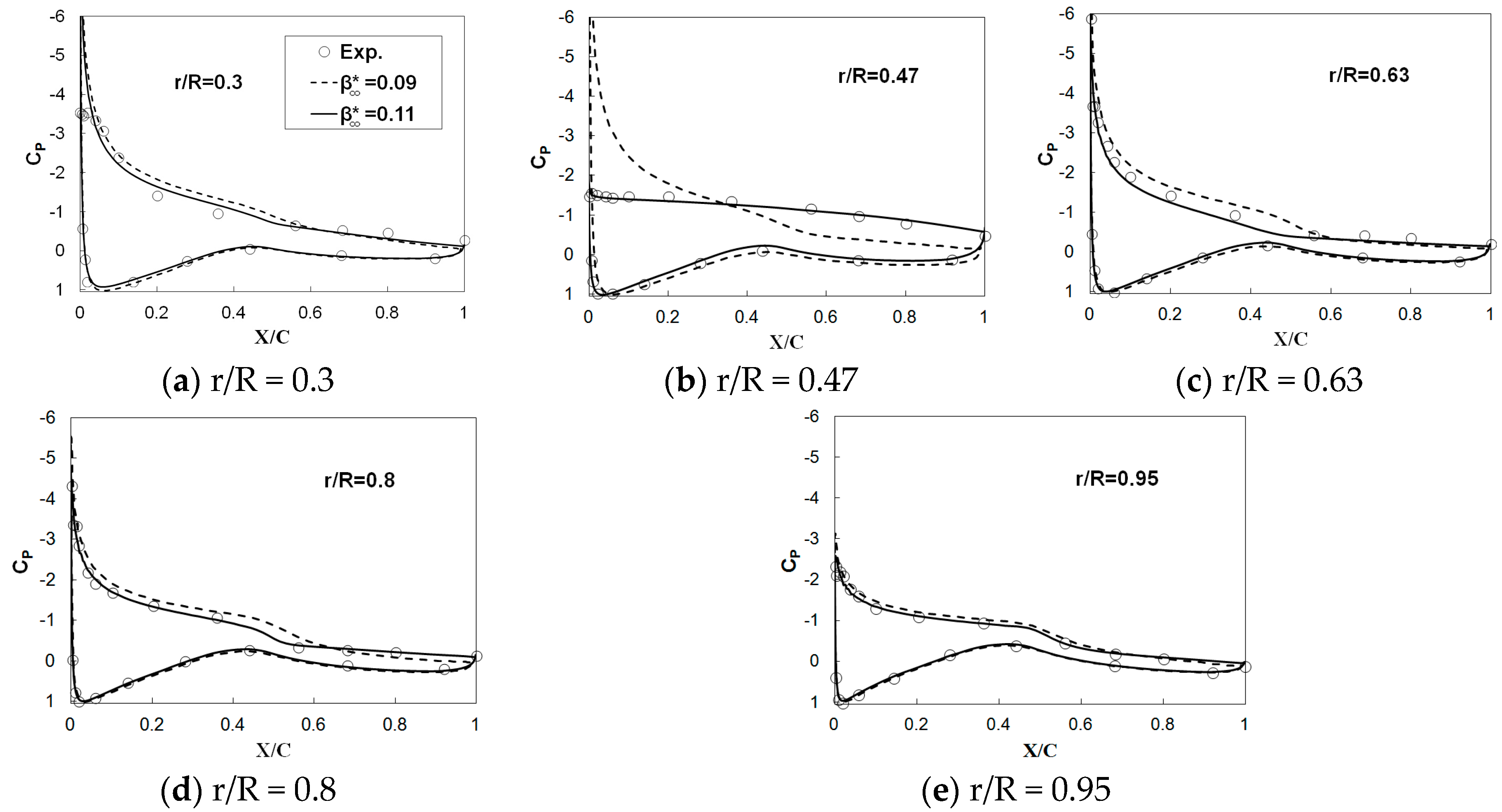
Figure 17.
The simulation results of pressure distributions for different values of , with a comparison to the measured data of the NREL Phase VI experiment. (Wind speed: 10 m/s).
Figure 17.
The simulation results of pressure distributions for different values of , with a comparison to the measured data of the NREL Phase VI experiment. (Wind speed: 10 m/s).
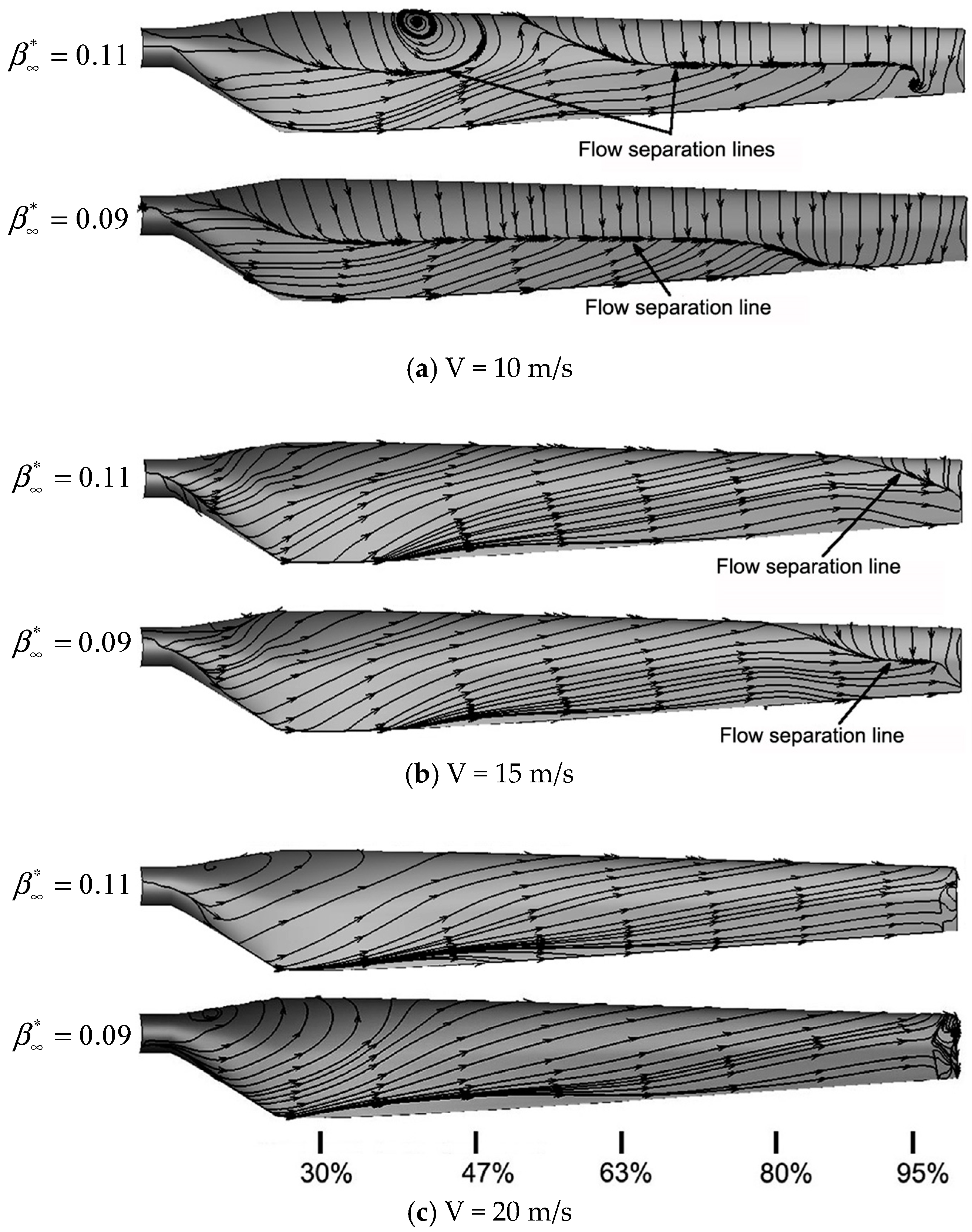
Figure 18.
The simulation results of limiting streamlines on the suction side of the blade, for different values of .
Figure 18.
The simulation results of limiting streamlines on the suction side of the blade, for different values of .
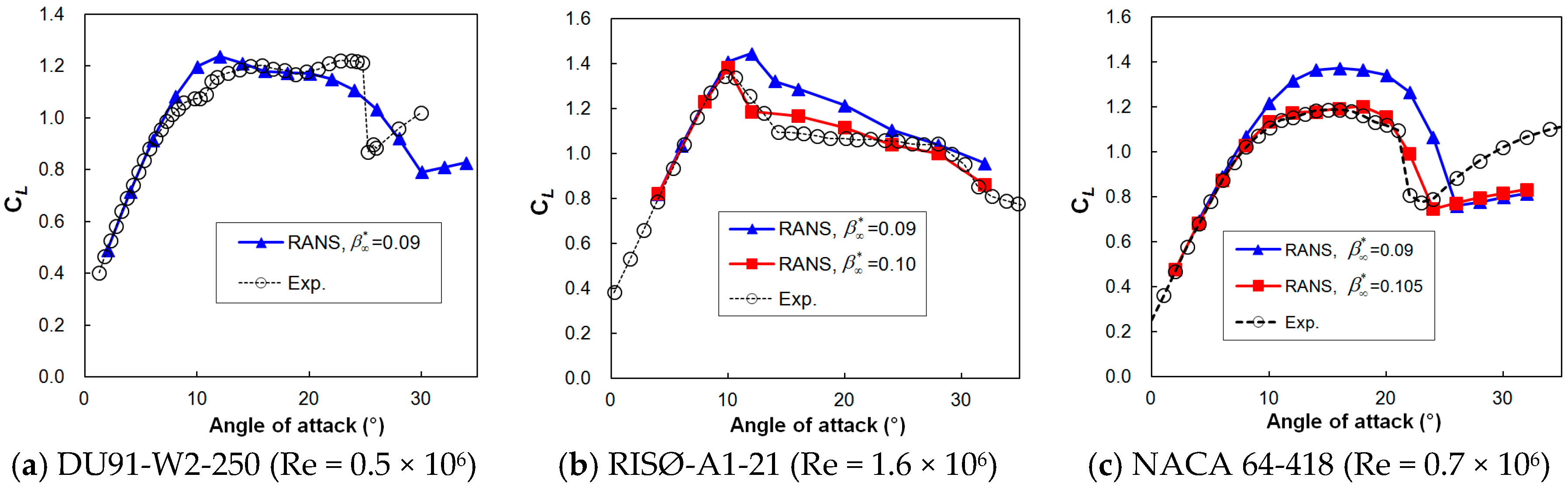
Figure 19.
The predicted lift coefficients of the airfoils DU91-W2-250, RISØ-A1-21, and NACA 64-418 for different values of , with a comparison to experimental data.
Figure 19.
The predicted lift coefficients of the airfoils DU91-W2-250, RISØ-A1-21, and NACA 64-418 for different values of , with a comparison to experimental data.
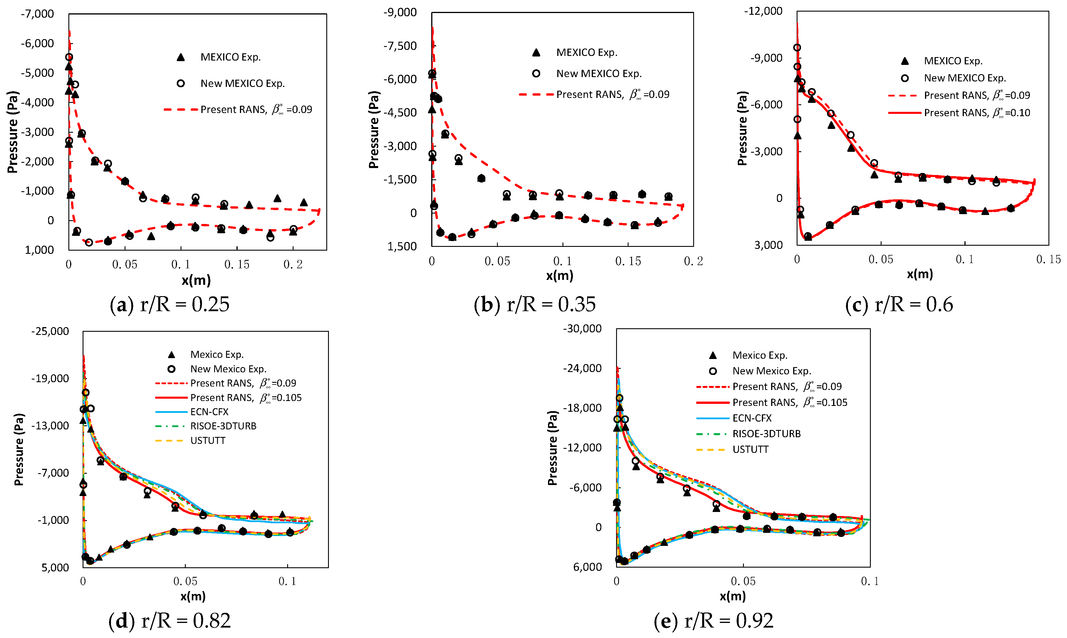
Figure 20.
The predicted pressure distributions over blade sections for different values of
compared to experimental data and a collection results of the Mexnext project [
29].
Figure 20.
The predicted pressure distributions over blade sections for different values of
compared to experimental data and a collection results of the Mexnext project [
29].
Table 1.
Computational settings of the airfoil simulation.
Table 1.
Computational settings of the airfoil simulation.
| Items | Options | Settings |
|---|
| | Space | 2D |
| Models | Time | Steady |
| | Viscous | SST k-omega |
| Pressure-Velocity Coupling | Type | Coupled |
| Courant Number | 50 |
| Discretization Scheme | Pressure | Second Order |
| Momentum | Second Order Upwind |
| Turbulent Kinetic Energy | Second Order Upwind |
| Specific Dissipation Rate | Second Order Upwind |
Table 2.
Computational settings of the rotor simulation.
Table 2.
Computational settings of the rotor simulation.
| Items | Options | Settings |
|---|
| Models | Space | 3D |
| Time | Steady |
| Viscous | SST k-omega |
| Motion type | Moving reference frame |
| Periodic type | Rotationally Periodic |
| Pressure-Velocity Coupling | Type | Coupled |
| Courant Number | 50 |
| Discretization Scheme | Pressure | Second Order |
| Momentum | Second Order Upwind |
| Turbulent Kinetic Energy | Second Order Upwind |
| Specific Dissipation Rate | Second Order Upwind |
Table 3.
The meshes involved in the test of mesh independency for the NREL Phase VI rotor.
Table 3.
The meshes involved in the test of mesh independency for the NREL Phase VI rotor.
| Mesh ID | M01 | M02 | M03 | M04 | M05 |
|---|
| Initial height of cells adjacent to blades (m) | 5 × 10⁻⁶ | 5 × 10⁻⁶ | 5 × 10⁻⁶ | 5 × 10⁻⁶ | 5 × 10⁻⁶ |
| number of Nodes along the blade span | 40 | 45 | 50 | 55 | 60 |
| number of Nodes along the blade chord | 140 | 190 | 240 | 290 | 320 |
| Growth ratio of grid size away from blade | 1.2 | 1.15 | 1.1 | 1.08 | 1.065 |
| Total number of cells (million) | 1.36 | 2.29 | 4.24 | 6.97 | 9.83 |
Table 4.
Results of the mesh independency study based on Richardson extrapolation 1.
Table 4.
Results of the mesh independency study based on Richardson extrapolation 1.
| Wind Speed | Mesh ID | Richardson Extrapolation |
|---|
| M01 | M02 | M03 | p | R* | TE |
|---|
| 7 m/s | 744.2 | 756.5 | 757.4 | 4.18 | 0.073 | 757.5 |
| 10 m/s | 1597.4 | 1778.6 | 1802.6 | 3.19 | 0.132 | 1806.5 |
| 15 m/s | 850 | 1309.5 | 1408.8 | 2.36 | 0.216 | 1439.1 |
| 20 m/s | 1047.6 | 1006.4 | 1001.4 | 3.33 | 0.121 | 1000.7 |
Table 5.
The flow patterns of five sections of the NREL Phase VI blade at various wind speeds.
Table 5.
The flow patterns of five sections of the NREL Phase VI blade at various wind speeds.
| Wind Speed | r/R = 0.3 | r/R = 0.47 | r/R = 0.63 | r/R = 0.8 | r/R = 0.95 |
|---|
| V = 7 m/s | No stall | No stall | No stall | No stall | No stall |
| V = 10 m/s | Light stall | Light stall | Light stall | Light stall | No stall |
| V = 15 m/s | Deep stall | Deep stall | Deep stall | Light stall | Light stall |
| V = 20 m/s | Deep stall | Deep stall | Deep stall | Deep stall | Deep stall |
Table 6.
The relative simulation error of lift coefficient for different values of .
Table 6.
The relative simulation error of lift coefficient for different values of .
| AoA (°) | 8 | 10 | 12 | 14 | 16 | 18 | 20 | |
|---|
| = 0.09 | 5.8% | 18.1% | 23.0% | 18.9% | 22.7% | 39.4% | 82.2% | 30.0% |
| = 0.11 | 2.2% | 1.3% | −0.3% | 0.5% | 6.1% | 17.5% | −3.9% | 4.5% |
Table 7.
The relative simulation error of the rotor torque for different values of .
Table 7.
The relative simulation error of the rotor torque for different values of .
| Wind Speed | 9 | 10 | 13 | 15 | 17 | 20 |
|---|
| = 0.09 | 4.7% | 34.4% | 29.0% | 20.2% | 0.6% | −9.8% |
| = 0.11 | −2.3% | 3.2% | −4.5% | −15.7% | −18.8% | −9.6% |
Table 8.
Information about the five sections and their Reynolds numbers in the present case.
Table 8.
Information about the five sections and their Reynolds numbers in the present case.
| r/R | r (m) | Chord (m) | Profile | Re |
|---|
| 0.25 | 0.563 | 0.224 | DU91-W2-250 | 0.38 × 10⁶ |
| 0.35 | 0.788 | 0.193 | DU91-W2-250 | 0.46 × 10⁶ |
| 0.6 | 1.350 | 0.142 | RISØ-A1-21 | 0.58 × 10⁶ |
| 0.82 | 1.845 | 0.113 | NACA 64-418 | 0.64 × 10⁶ |
| 0.92 | 2.070 | 0.099 | NACA 64-418 | 0.62 × 10⁶ |


