1. Introduction
The world energy demand has been increasing exponentially while conventional energy resources are exhaustible and limited in supply. Therefore, there is an urgent need to conserve the energy resources that are at hand and explore alternative energy resources. Among the various types of renewable energy sources (RESs), solar and wind energies are the most promising sources. Recently, the use of RESs in the form of distributed generators (DGs) and distributed energy systems (DESs) [
1] has increased with the aim of an environmentally-friendly society. Moreover, these DGs can supply energy in an isolated situation [
2,
3,
4]. However, RESs output is influenced by weather uncertainty, causing voltage deviation, fluctuation and reverse power flow under a high penetration of DGs using RESs [
5]. The conventional provisional method for voltage fluctuation is often handled by the use of an on-load tap changer (OLTC) transformer such as the load ratio transformer (LRT) and the step voltage regulator (SVR). This method is only effective for slow changes in voltage by switching the primary and secondary winding ratios of the transformer. Thus, this method cannot maintain the voltage well because steep voltage fluctuations are the nature of the DGs. In addition, voltage regulation by OLTC has not reached a fundamental solution for power quality considering the power factor. As a countermeasure to this problem, the use of reactive power controllers, such as additional static VAR compensators (SVCs) [
6,
7,
8,
9,
10,
11] or the reactive power control system by the inclusion of an inverter with distributed generators [
12,
13,
14,
15,
16,
17,
18] has been proposed. The literature [
19] has discussed rapid and precise tap control online. Another proposed reactive power control improves voltage maintenance and the utilization rate of equipment of the system, which is utilizing the empty area of inverter capacity of an interfaced inverter of an RES generator and battery energy storage system (BESS) [
20]. Thus, reactive power compensation methods can be categorized into two types, which are the use of devices at the distribution company (DisCo) side or utilizing the customer side inverter. In particular, using an introduced large capacity BESS at the substation and reactive power output from customer DGs avoids reverse power flow and voltage fluctuation.
An increase in demand and a massive installation of RES with uncertainty frequently causes an imbalance in the power system within hours. It is essential to improve forecasting techniques to solve the imbalance of demand and supply, but prediction accuracy cannot always be raised to 100%. Thus, in order to resolve power imbalance with RESs, the BESS has been installed and operated based on optimal scheduling in several areas. Scheduling of the distribution system has been proposed in much of the literature [
21,
22,
23,
24]. In addition, power quality such as the power factor has been improved by the reactive power control method using an interfaced inverter of BESS. The BESS can be introduced to the power system to compensate for power quality loss and fluctuations in voltage and frequency [
25,
26]. With the increase in the expectation of battery utilization to overcome all variations of RES output, the introduction cost becomes large, and the battery has to be introduced into various places according to DG load points. With the increase of batteries, the cost of the interfaced inverter tends to increase. In this trade-off relationship, it is required to optimize the capacity or capacity reduction of the storage battery.
Along with the limitation of control from the upper system, hence, it is proposed to obtain the balance that is controlling and regulating a load demand as the demand response (DR) [
27], and the non-cooperative game has been analyzed in the literature [
28]. Providing various pricing scheme (e.g., time of use (TOU), real-time pricing (RTP)) means it consciously changes the net load usage and intentionally levels the active power profile of the customers in the DR program. Furthermore, ancillary services of DR secure reserve power, which is effectively supported by battery storage from power security. In order to reach an effective use of BESS and renewable DGs, distributed energy resources management systems (DERMSs) provide the management matching system requirement for a sustainable society associated with the smart meter on the customer side [
29]. The DR might be incorporated in the DERMS. The DR mainly brings benefits to the power company such as the generation company (GenCo) and distribution company (DisCo), so it is not for the customers. By optimizing the operation using the smart meter, some users can reduce power purchase cost. A participative DR program affects electricity consumption; however, this means some options of the program (e.g., interruptible load, load shedding) force one to change the usage of the power schedule. The customer feels dissatisfied with suppressed power consumption by pricing or other DR programs.
Based on the above recent activity regarding the power system, we will summarize the issues considered in this research as follows:
Technical issues related to high penetration of RES (voltage deviation and reverse power flow)
Cost increase due to increased controllers and storage battery for voltage control and surplus power absorption.
Issues for the DR program; increase in dissatisfaction with small demand response due to price change and compulsory DR.
Proposing a balanced system construction is important while securing the benefits of both DisCo and consumers.
Contributions and Structure of This Paper
Recently, the use of customer-side inverter compensation methods has been shown to be more economical in comparison with the installation of additional SVC devices due to the high penetration of DGs and inverters with DGs. However, voltage control of this proposed method [
30] depends on an adequate reactive power output from the customer (player in game theory). If customers do not provide the reactive power requested by the distribution company (DisCo) to the grid, the distribution system will be unstable due to large voltage fluctuations. In order to obtain proper reactive power output from the customer, the DisCo should frame the system in such a way as to encourage the customers to follow DisCo requests.
Therefore, this paper proposes a system called the reactive power incentive system. The system is intended to encourage customers to output the appropriate reactive power as requested by the DisCo by allowing them to obtain rewards corresponding to the reactive power requirement of the DisCo. If customers output the proper reactive power, some burden of the DisCo, such as the need for reactive power compensators or LRTs and SVRs, will be mitigated. The compensation that the DisCo pays to its customers is covered by the burden that has been alleviated by coordination with the customers. By using this proposed method, the DisCo can save on costs due to mitigating the burden of some control equipment; customers also get the advantage of incentives by following suitable reactive power output regimes as requested by the DisCo. This reactive power DR program serves to improve the power quality of the power system without requiring a change in normal load consumption, as compared with a conventional DR handling only active power. The effectiveness of the proposed method is confirmed using MATLAB® simulations. Not only does this paper provide a detailed technical assessment, but it also shows the economic benefits of both of the DisCo and customers. In addition, optimal operation is calculated by using the particle swarm optimization (PSO) algorithm, and the solution is provided as optimal one-day scheduling. In order to avoid over-control, a modified scheduling method is proposed in this paper.
The paper is organized as follows:
Section 2 explains DR regarding active and reactive power. In
Section 3, in order solve the problem of high penetration of DGs using RES causing voltage deviation and reverse power flow, formulations of the distribution model, objective function, optimization method and control device configuration are provided. The method of reactive power incentive is provided in
Section 4. The optimization algorithm and modified scheduling method are explained in
Section 5. In
Section 6, the simulation results are presented as case studies.
Section 7 concludes this paper.
2. Demand Response
DR programs are proposed in many countries to solve some of the issues of urgent concern in power generation, especially in developed countries. The details of the DR mechanism on price have been discussed in [
31,
32,
33], the research of which revealed the structure between the aggregator and customer relationship, as well as the incentive profit and penalty based on the behavior of changing consumption. DR management of load shedding by directly controlling the turning on/off of device load was proposed as a smart direct load control with the recent Internet of Things (IoT) technology [
34].
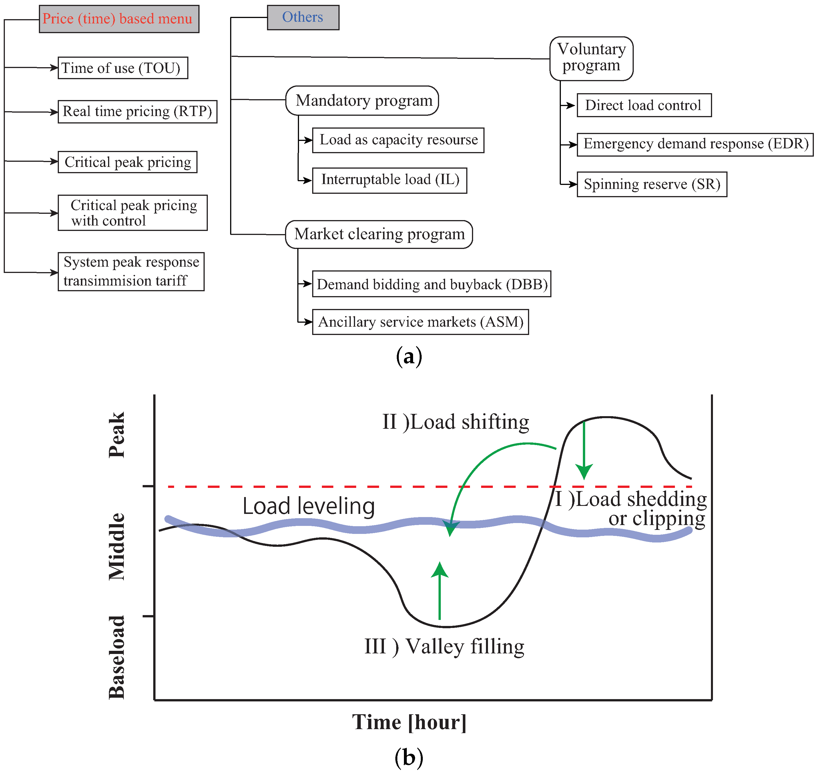
In the electricity market, a DR configuration consists of some menu (e.g., pricing, market-based DR, physical basis (load), etc.) The DR can be categorized as mandatory, voluntary and based on contract, to name a few, as in
Figure 1a [
35]. Most cases of DR suppress load demand at a peak time and shift usage time. It is then desirable to level the load profile in the DR program as shown in
Figure 1b. Here, in order to show the influence by the pricing-based DR purely, the consumer’s willingness to change the demand for the change in the electricity price excluding the operation of the storage battery, etc., will be explained.
2.1. Price Elasticity
Under the condition that the DR has been carried out, load flexibility and the ability of responsive capacity are shown by the price elasticity of demand. The price elasticity of load demand is expressed as follows [
35,
36]:
According to Equation (
1), the price elasticity at term
i,
j (24 h) can be defined as [
35]:
Considering price elasticity at time i corresponding to j, it could the express schedule of load usage regarding shiftable load under the DR event. In the case of reduced load, it is represented by the price elasticity of negative value and vice versa.
Electricity usage has penetrated everywhere, falling into the lifeline of essential goods and services. Therefore, the customer is not sensitive to changing the unit price of electricity, and at present, one can only expect price elasticity of about −0.1 [
37]. In other words, DR based on price is not a big adjustment of power in negawatt trading [
38], and DR that forces load reduction is a cause of dissatisfaction.
2.2. Reactive Power Market
Reactive power control is an important technique for maintaining the power quality of voltage and power factor improvement. In recent years, due to the improvement of IoT technology, a system capable of giving and receiving reactive power from distributed power sources and household inverters’ unused capacity has been proposed. Therefore, a reactive power market has been proposed, which buys and sells with respect to reactive power not normally consumed [
39,
40]. However, the reactive power market is not opened for end-users of the power system. Y.Han et. al. [
41] have discussed reactive power sharing in microgrids with IoT technology. Against this backdrop resulting from IoT development, the mechanism that various customers can participate in for reactive power control is becoming a reality, but there are few papers that have discussed the incentives and benefits that they offer.
3. Modeling and Formulation for the Optimization Problem
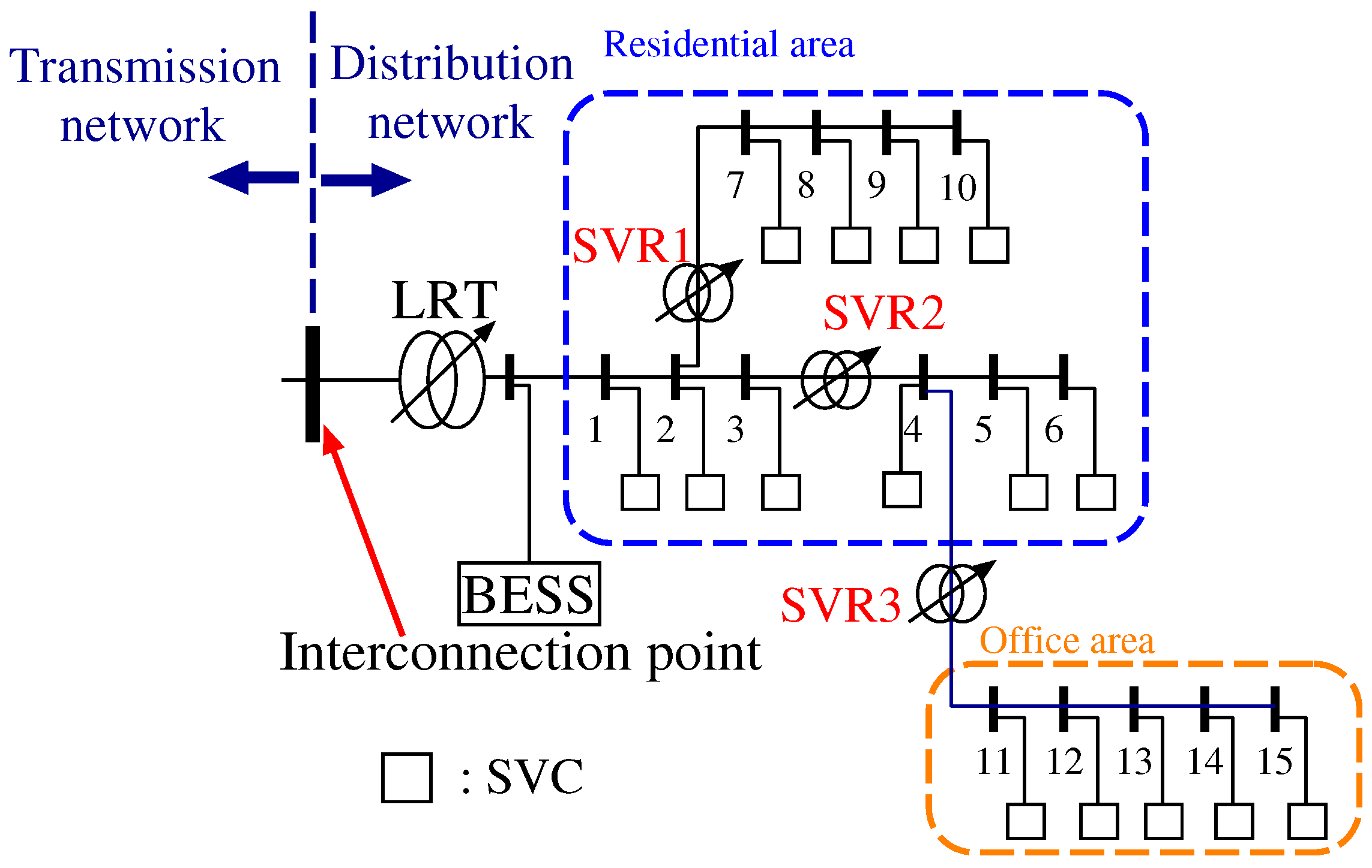
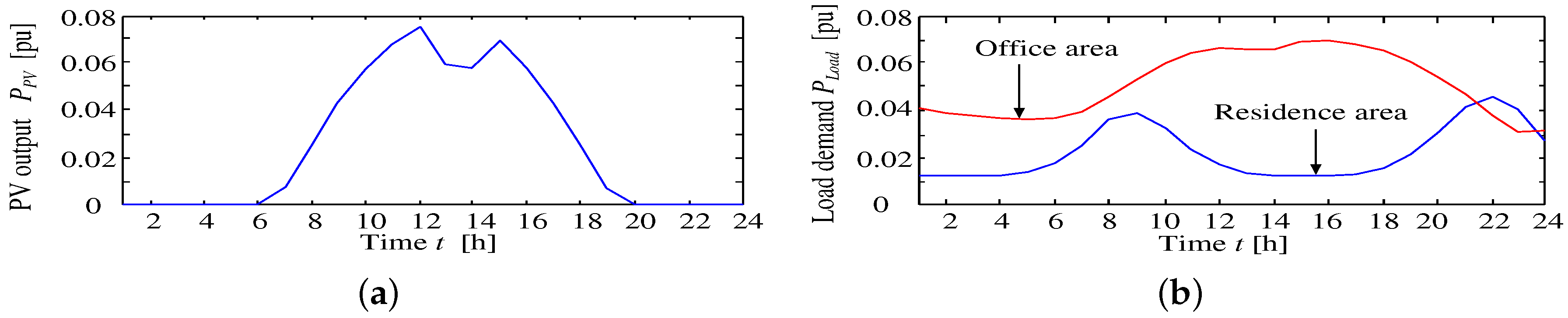
In this paper, the distribution system consists of a substation with LRT and 15 customer-side nodes. These nodes can be divided into two types of areas, which are the residential and office areas shown in
Figure 2. PV generators and SVCs are installed at all nodes in the distribution system, and parameters related to the distribution system are listed in
Table 1, where the nominal capacity and the nominal voltage of the distribution system are 5 MVA and 6.6 kV, respectively. This section describes the decision technique for the tap changing of existing voltage control devices (LRT), the reactive power control method using inverters interfaced with the PV and BESS control at the interconnection point, instead of reactive power supply from SVC and SVR tap ratio control.
3.1. Objective Function and Constraints for Optimal Scheduling
In order to adapt the optimization method to the described problem, the objective function and constraints are determined as described in this section. Here, the control devices are the BESS, BESS-interfaced inverter, PV-inverter and tap control transformers.
Objective function:
The objective function for conventional scheduling can be represented as follows:
The objective function
is used to minimize the distribution losses for a period of one day.
,
,
,
are determined as control variables.
means the number of distribution nodes. This function is used to find the optimal reference value of cooperative operation. In the proposed incentive approach, the objective function is updated as follows:
3.2. Constraints
Robust voltage range for PV installation:
Generally, all nodes’ voltage constraint is expressed as Equation (
5):
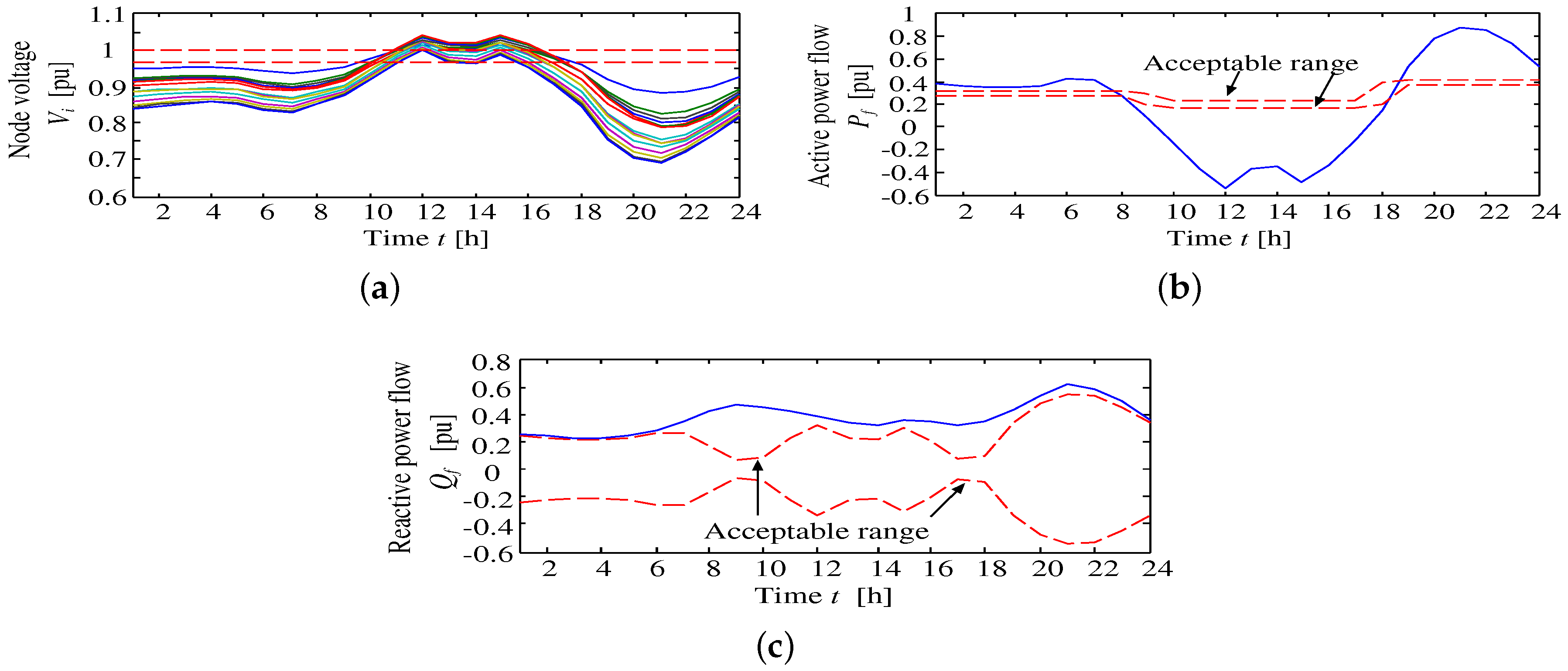
A stipulated voltage range of a low voltage distribution area under a pole transformer is set to be within 101 ± 6 V in the Electricity Act of Japan. According to [
20], the distribution voltage will fluctuate up to 6.5 V in a low voltage area under the high penetration of RES. In order to preserve robustness, thus a restriction has been put on the general voltage limit (95–107 V) as 101.5 V–105 V in this work. By configuring all pole transformers at a transformation ratio of 6600 V:105 V, the
and
are assigned 6380/101.5 V (0.967 pu) and 6600/105 V (1.0 pu), respectively.
Power flow constraints regarding reverse power flow and the power factor:
The active and reactive power flow constraints at an interconnected point are written as follows:
To compensate for reverse power flow in the static simulation, a flexible boundary is set as the active power flow. In order to avoid unnecessary use of control devices, the active power flow limit is shaped in such a way that a lower amount of control is necessary. Distribution losses also depend on power flow fluctuation; hence, the bandwidth of active power flow is set to
pu. It is essential to note that the bandwidth and shape should be set by considering the installation rate of PV amount and the load curve profile. On the other hand, the acceptable range of reactive power flow considers the power factor (PF) value, which depends on active power flow [
42].
The PF of the interconnection point is maintained from 0.85–1.0. Reactive power flow limits are determined from the active power flow value. Thus, the upper and lower reactive power limit are rewritten as follows:
BESS configuration and operation:
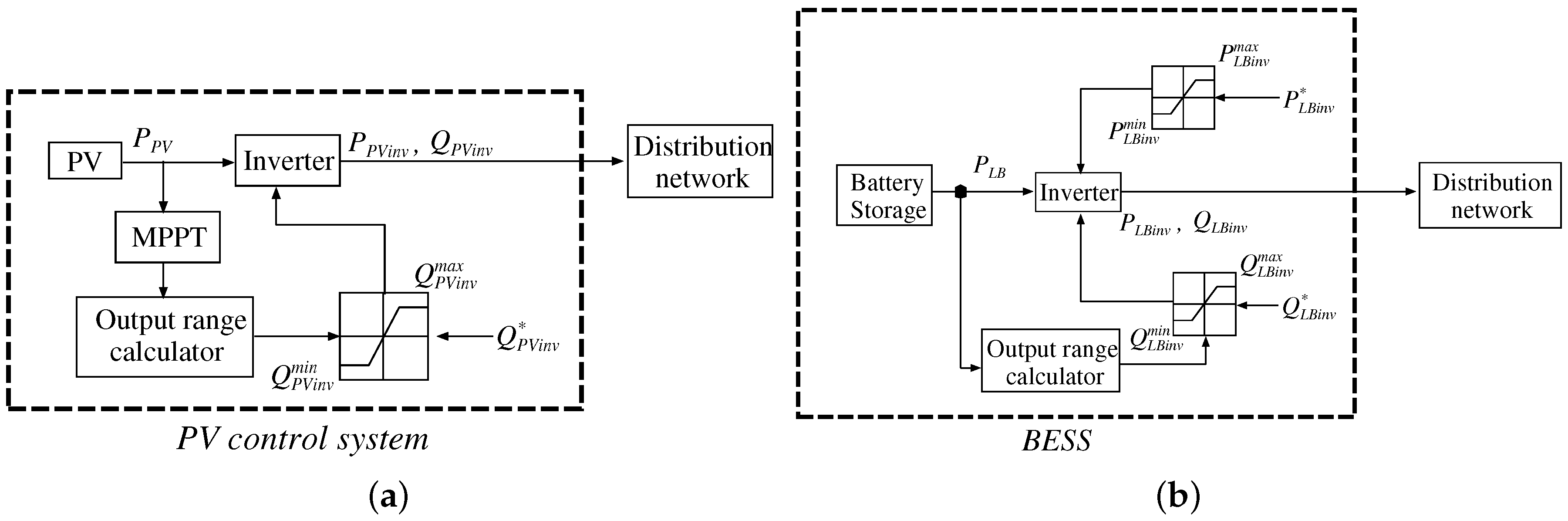
To suppress large fluctuations of power flow at the interconnection point, the power flow constraint is supported by using the BESS at the substation. The power controller of BESS is shown in
Figure 3b. The optimized control reference signal is generated based on the forecasted information. In this paper, the BESS is assumed to have NASbatteries; the charge/discharge efficiency of the BESS is 80%; whilst the self-discharging of the BESS is not considered. These constraints are described as follows:
These equations are constraints regarding the large capacity BESS, considering battery SOC and the efficiency of charging and discharging.
PV system:
DGs using PV have a simple configuration and maintenance-free characteristics. Details of the PV cell and its inner structure are described in [
43]. For utilization improvement of the PV system in an ever-changing climate, it is assumed that the PV system has the maximum power point tracking (MPPT) algorithm. The reactive power control scheme utilizes capacity margins of the installed PV inverter shown in
Figure 3a. The inverter constraint is defined as Equation (
11):
The feedable reactive power from the PV inverter is rewritten as follows:
Here, the amount of
is the main factor for cooperative operation, which is discussed in
Section 4.
OLTC tap constraints:
The OLTC concludes the LRT and SVR, the tap positions’ constraint of which is given by:
In LRT operation, short-term operation is undesirable. Thus, LRT can control at a rate of one tap-step ratio in one hour. The tap position variable is discrete. Therefore, the optimization problem is known as a mixed integer non-linear problem (MINLP).
4. Reactive Power Incentive Method
DR methods can be roughly classified into two categories, such as TOU type and incentive type. DR using the TOU method depends on the electricity price [
27,
44], which encourages the customer to change the usage of electric power. On the other hand, incentive-based DR is independent of electricity price, in which a customer can earn a profit from DisCo by the cooperative operation process. The customer side does not need to change the usage of power. Generally, DisCo has to invest in maintaining the power system, and the investment costs include equipment, maintenance and operation, which becomes a burden to the DisCo. However, these costs can be reduced through the cooperative operation of the customer side. A cooperative operation system is possible with HEMSsmart grid technology [
45,
46,
47,
48]. The reactive power incentive concept provides an amount of profit to the customer to contribute to the sustainable power system of DisCo. If all customers follow the DisCo’s request for the specified reactive power output
, the DisCo can remove the unnecessary burdens of equipment costs. Therefore, the DisCo can provide incentives from saved money to customers participating in the cooperative operation program.
4.1. Calculation of Reactive Power Incentive Unit Price
Reducing the cost of voltage control devices through the cooperative operation of the customer can be described by Equation (
14). This equation includes SVR and SVC costs.
and
are set to 15 and three, respectively. These numbers of devices are required when this case is considered without cooperative operation.
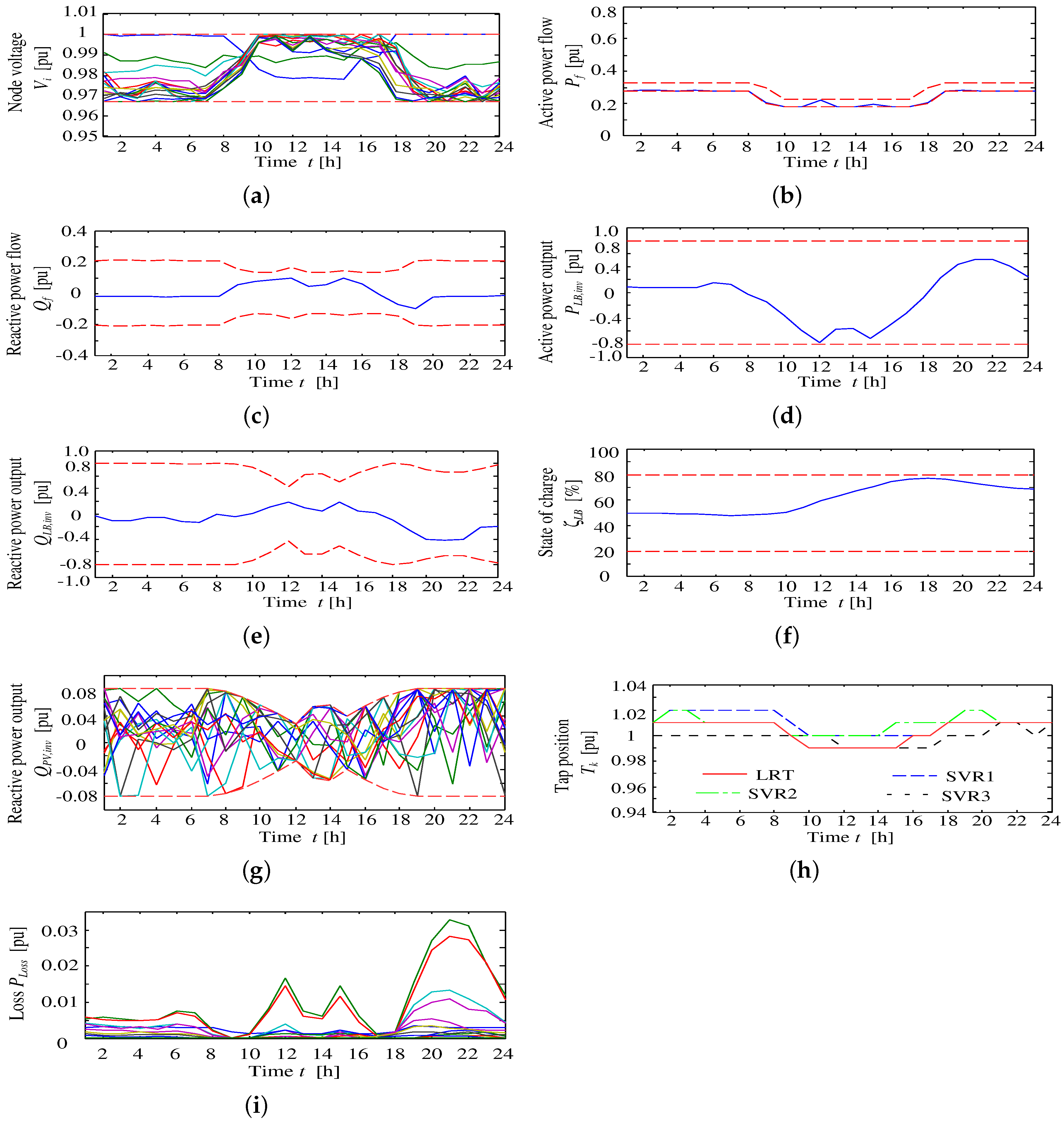
Figure 2 shows SVR1, SVR2 and SVR3, which are located between Nodes 2 and 7, between Nodes 2 and 3 and between Nodes 4 and 11, respectively.
By considering the depreciation term and total costs,
can be obtained from the following equation:
The depreciation term
is determined for 20 years. SVC and SVR costs are displayed in
Table 2, and also, SVC capacity and reactive power unit price are listed in
Table 2. Because the
should distribute to all customers, the value is derived by the number of branching nodes in the distribution system.
4.2. Contribution Factor
DisCo pays incentives for requesting reactive power cooperation. Due to the decision of the incentive amount, DisCo has two processes to assess the contribution; (1) decide and notify based on the day-ahead scheduling, (2) the contribution factor is calculated based on the difference between and the provided reactive power .
The proper value
is generated by solving Equation (
16):
Then, consumers are requested to use the optimal reactive power amount allocated as the reference value for the proposed DR event. Consumers can then make a contribution to reactive power if they can provide a value close to this reference value for the cooperative control. DisCo calculates the contribution rate according to the consumer’s reactive power supply amount. In this work, linear and sigmoid functions have been developed to calculated the contribution factor.
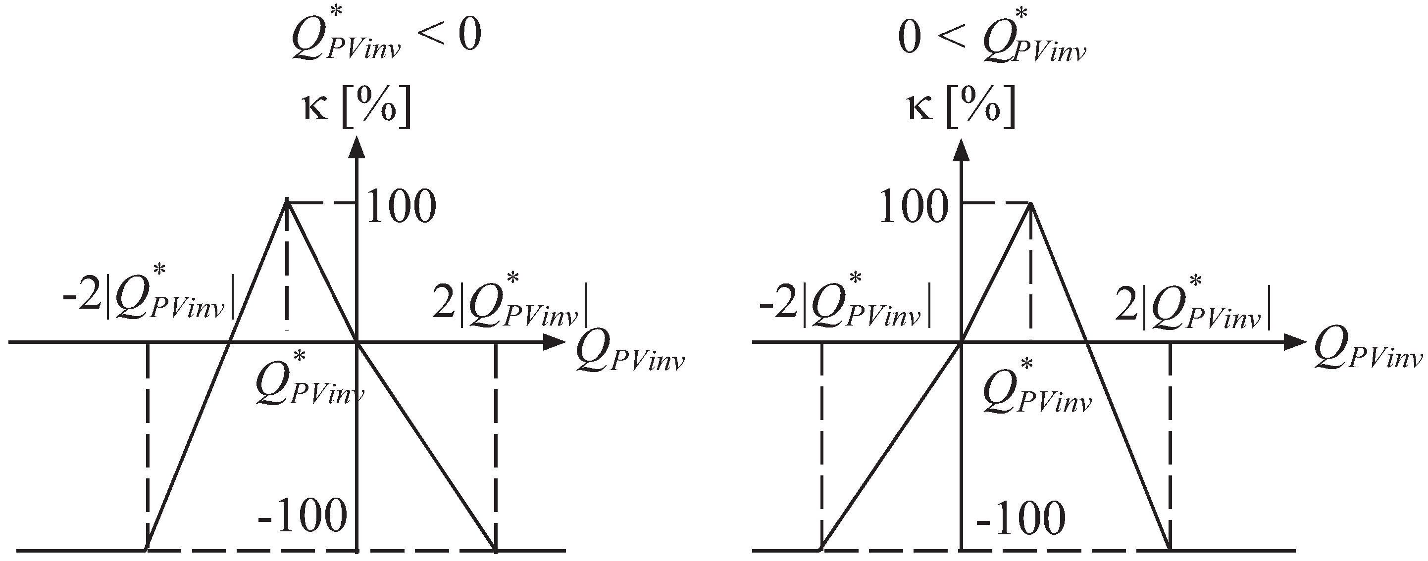
Linear contribution function:
The contribution rate defined as a linear function is shown in
Figure 4, in which the slope of the linear contribution function is generalized as follows:
Then, the contribution factor is determined as follows:
When the indicates a negative value, the participating customer will have a penalty applied.
Sigmoid function:
The contribution factor is written by applying the sigmoid function as:
where coefficient
determines the shape of sigmoid function, whenever Equation (
19)
.
is given by solving Equation (
19) for each time step
t:
Here,
is the contribution reference value when DisCo obtained
. Furthermore, in order to determine the proper reactive power contribution,
is assigned in the work, since
. The sigmoid contribution factor is given by substituting
into Equation (
20), yielding:
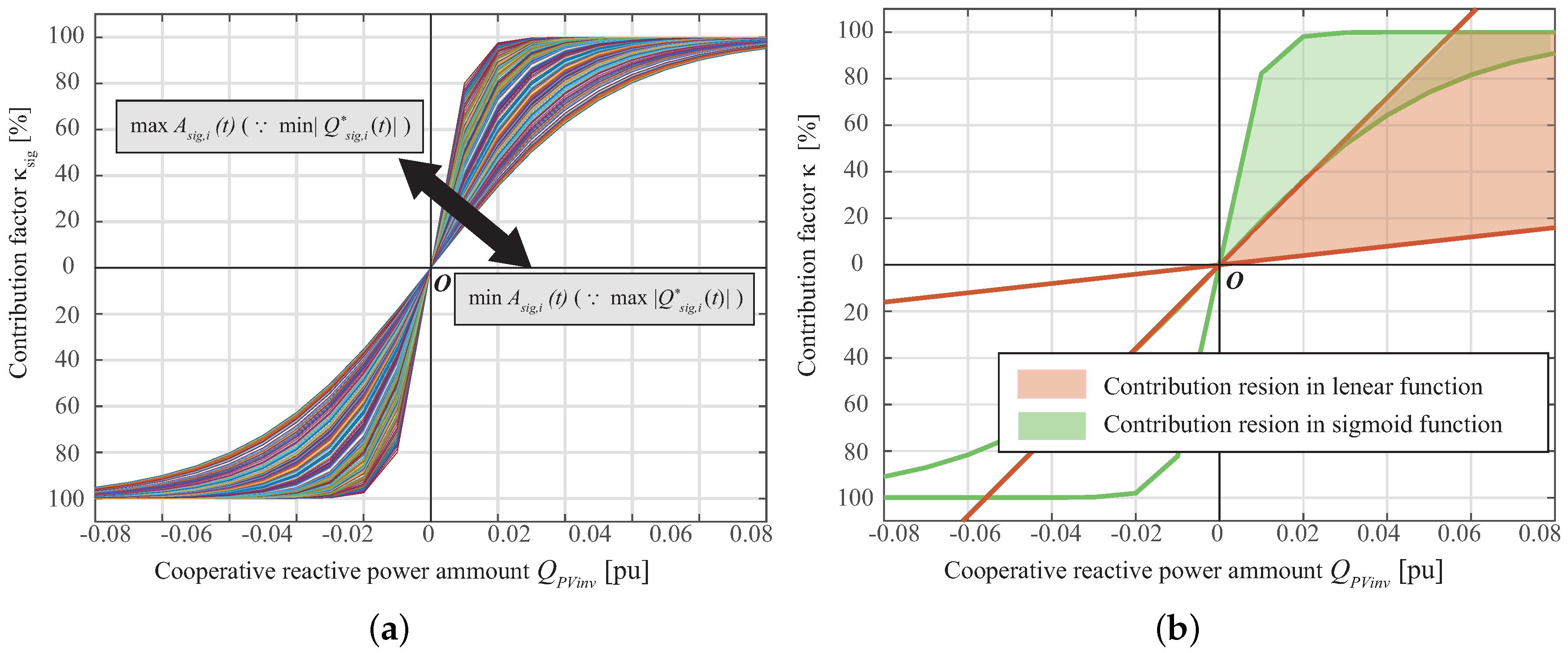
The
is plotted against several reference values
in
Figure 5a. A feasible region comparison for linear and sigmoid contribution functions is illustrated in
Figure 5b.
4.3. Profit Obtained by Customers
Once
is determined, customers can calculate their own obtained profit
following the order from DisCo. The
is disclosed in
Figure 4, and the profits obtained by the customers can be derived using Equation (
22).
In this paper,
is 5000 kW.
is the reactive power incentive considering the contribution factor
, and it is described by the following equation:
Therefore, customers can obtain a maximum profit by supplying reactive power output close to . Since all customers should carry out the command for maximizing the profit, DisCo can maintain the voltage using this incentive.

 ,
, 


