Mode Profile Shaping in Wire Media: Towards An Experimental Verification
by
 , , and
Taylor Boyd
1,2,3, 
Jonathan Gratus
1,2,*,
Paul Kinsler
1,2,
Rosa Letizia
1,3 and
Rebecca Seviour
4 1
Cockcroft Institute, Sci-Tech Daresbury, Daresbury WA4 4AD, UK
2
Physics Department, Lancaster University, Lancaster LA1 4YB, UK
3
Engineering Department, Lancaster University, Lancaster LA1 4YB, UK
4
Department of Engineering and Technology, University of Huddersfield, Huddersfield HD1 1JB, UK
*
Author to whom correspondence should be addressed.
Appl. Sci. 2018, 8(8), 1276; https://doi.org/10.3390/app8081276
Submission received: 18 July 2018
/
Revised: 26 July 2018
/
Accepted: 28 July 2018
/
Published: 1 August 2018
(This article belongs to the Special Issue Photonic Metamaterials)
Abstract
:We show that an experimentally plausible system consisting of a modulated dielectric wire medium hosted in a metal cavity or waveguide can be used to shape the longitudinal field profile. In addition, a more realistic permittivity is used. These new frequency domain numerical results are a significant step towards justifying the construction of an experimental apparatus to test the field profile shaping in practise.
1. Introduction
Spatial dispersion is a valuable tool, which can be used to customise the profiles of electric fields in metamaterial and photonic structures. As we have already shown [1,2,3], such field profile customisation is even possible at the sub-wavelength scale, and does not require exhaustive brute-force computation. Further, for our spatially dispersive wire medium [3], we show this system can support shaped longitudinal electric fields. This field profiling is achieved by varying the radius of the wires in a carefully calibrated way. In [3] the system was numerically modelled as an infinite periodic array of wires, so that the computation only required a single wire with periodic boundary conditions. In addition to periodicity, the simulated wire material had a very high permittivity and concomitantly small radius, features that would be problematic in experiment, both in terms of manufacture and fragility. Nevertheless, we did show that such extreme structures were not necessarily required, since re-scaled calculations indicated the shaping effect would still persist even with lower permittivities and larger wire radii.
Such field profiling has a variety of potential uses. The idea has been implemented by means of harmonic synthesis [4,5], and suggested in the context of nonlinearity-induced carrier shocking [6,7,8]. Such shaped waveforms have been suggested as a means of enhancing ionisation in high harmonic generation [9,10]. Other shapes could find uses, such as fields with locally high gradients but without a large peak-minimising nonlinear effects, or fields with pronounced peaks and low amplitude elsewhere to improve signal to noise ratios. In particular, we are interested in accelerator applications where the field profile might be used for electron bunch shaping, or as part of a laser wakefield accelerator [11,12]. This requires us to improve on our initial idealised simulations and incorporate experimental features such as more realistic material choices and a supporting waveguide systems.
In this article, we show that the field profiling of a longitudinal wave predicted in [3] can be numerically reproduced in an experimentally plausible system. In [3] we considered an infinite periodic array of infinite wires as shown in Figure 1, where the wire radius varied from to with a relative permittivity of . As longitudinal electromagnetic waves (EM waves) are known to exist in guided wave systems we consider a array of finite-wires, a single period long, and contained in a metallic waveguide closed at both ends, as depicted in Figure 2. In the simulations reported here, our wire parameters are physically easier to realise than those used in [3], being based on a wire radius that varies from to , with a relative permittivity of . The simulation of this system was undertaken using the frequency domain solver of the commercial software CST Microwave Studio (2018 Update, Framingham, MA, US).
As in [3] we concentrate on sculpting the electric field profile based on the periodic Mathieu function
where L is the field wavelength, and the period of variation in the wire radius is . This field profile has a flatter maximum than a sinusoid, and a steeper gradient when passing though zero. The Mathieu functions are the solution to the differential equation
The periodic solution in (1), is given when , and .
2. Modulated Wire Media
This work is based on the understanding of wire media, a class of metamaterials consisting of a regular (rectangular) array of parallel wires or rods, whose radius is small compared to their spacing [13,14]. When the wire radii also vary, such three-dimensional inhomogeneous media are difficult to analyse in the absence of a simpler model for the system. Fortunately, the fixed-radius case is understood [13], which provides us with a starting point.
Any (fixed-radius) wire medium has an electromagnetic dispersion which follows the hydrodynamic Lorentz model, with a dependence on a resonance frequency, a polariton velocity, and a plasma frequency. In [3] we showed that, in effect, we could assume this held for any thin transverse slice of a wire medium. Thus, by stacking different wire radius slices together, to form not a uniform but a varying wire, we would construct a medium where the plasma frequency changed with position. This varying plasma frequency then leads to a correlated change in the effective local refractive index, thus—according to the electromagnetic wave equation—also changing the local curvature of the electric field profile. Since this curvature control changes the shape of the resulting wave, we can calculate how to link any desired field profile to a variation in wire radius.
This procedure, despite its efficiency, is still reliant on numerics. The analytic calculation of Belov et al. [13] was for infinitely thin wires, and so lacked the radius dependence we rely on to control their spatially dispersive properties. However, once we complete the step of numerically characterising a set of finite radius wires covering a suitable range of sizes, we can easily extract the necessary radius dependence of the plasma frequency. Please note that although the other hydrodynamic Lorentz parameters fitted to the numerical results do change, they are much less sensitive, and so that variation can be reasonably ignored.
3. Modulated Wires in A Supporting Waveguide or Cavity
For either an experimental configuration or a technological application, we would not expect to be able to use an unsupported array of wires in free space. Instead, we would need to use a finite array of wires in a supporting structure such as a metal waveguide or metallic cavity. Further, we would need to arrange the wires within that support so that the longitudinal field structure and the ability to sculpt the profiles is not disrupted or lost.
We choose to model a supporting structure that consists of either a metallic waveguide or cavity, aligned with a rectangular array of wires with varying radius. This leaves several design parameters to consider, (a) the (minimum) number of wires to place in the waveguide or cavity; (b) the distance of the waveguide or cavity side-walls parallel to the wires from the nearest wire, and; for a cavity, (c) the separation of the cavity end-walls perpendicular to the wires and their placement with respect to the modulation of the wires.
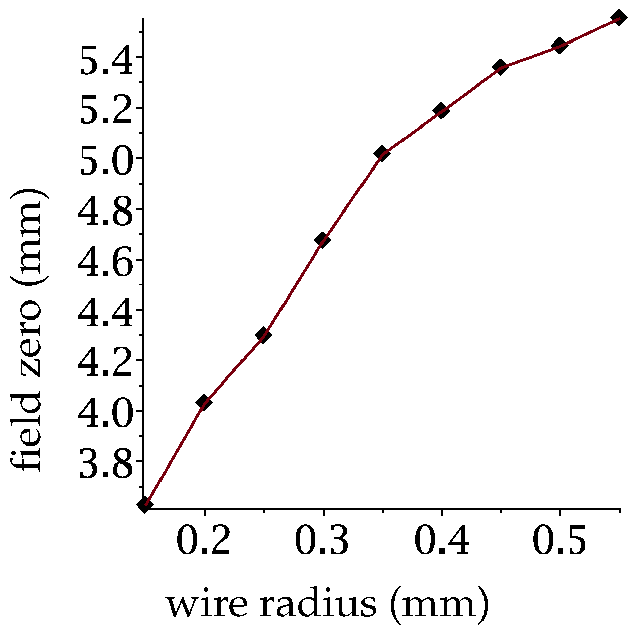
Given that the original simulations [3] were for an infinite periodic array of wires, we might expect that a large array of many wires would be necessary. However, we will see below that good results can be achieved with only a array; nevertheless in this article we concentrate on a array as we expect it may offer experimental advantages. Given such a finite array, we now need to consider the positioning of the side-walls, which would ideally be placed where the longitudinal field is small. Please note that in Figure 3c we see there is an approximately circular region around the wire where the (longitudinal) is zero. However, the contour is not only curved in contrast to the planar side-walls of our waveguide or cavity, but its distance from the wire varies with the wire radius as shown on Figure 4. Nevertheless, a reasonable compromise is possible since it turns out only requiring is sufficient.
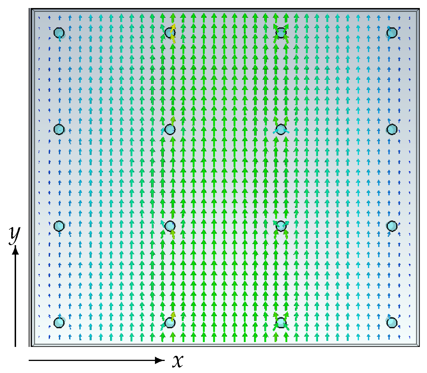
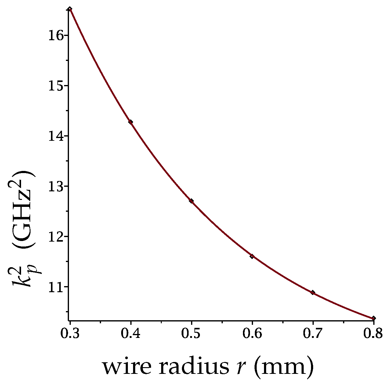
The first step when using our algorithm, detailed in [3], is to check that our proposed waveguide containing a array of uniform wires does indeed support longitudinal modes. As can be seen on Figure 5, strong longitudinal fields are indeed present in the centre between the inner wires. Next, we need to calculate the relationship between the wire radius r and the plasma frequency , and the results are shown on Figure 6 for the case. Our exponential fit to that data is used simply because it provides a good match to the data – as yet we have no theoretical reasons for the behaviour, although the accuracy of the fit strongly suggests that an explanation could be found. Note, however, that as we are modelling dielectric wires, it is not straightforward to apply arguments based on the Drude model and free carrier concentrations. For our chosen field profile, we use this information to calculate the generating radius variation, as seen on Figure 7. This produced a shaped longitudinal field shown in Figure 8, and which is compared with the desired profile on Figure 9.
The next step was to consider the case of a cavity rather than the infinite wavguide which requires us to choose where to place the perpendicular end-walls. In this case we made the straightforward decision to place them where the field has a symmetry, i.e. at its maximum and minimum values. Thus the cavity contains an exact half wavelength of the field, which is the same as one full period of the wire variation. We see in Figure 10 that the longitudinal profile of the mode is unaffected and from Figure 11 that the simulated field profiles is still in very good agreement with the intended Mathieu profile. We also repeated the above procedure for the simpler cavity with only a wire array, as shown on Figure 12 and Figure 13. Even in this reduced situation there was still excellent agreement with the desired electric field profile.
4. Frequency Isolation
When attempting to experimentally demonstrate profile shaping it is necessary to not merely excite the appropriate mode in the structure, but also excite only that mode. In particular, we need to be able to avoid exciting the nearby modes which may not be longitudinal, nor be correctly shaped. To assist with this selection, in Table 1 we show an eigenmode analysis for the cavity in the vicinity of the index 90 ( GHz) mode we wish to excite. At first sight this does not look promising, with nearby modes being within 0.1% (i.e. about GHz). However, we can also see that the nearest modes are transverse (as in Figure 14) rather than longitudinal, so that they should not be strongly excited as long as we only attempt to excite the desired mode with a well designed source. The nearest unwanted longitudinal mode is further away in frequency (about 0.9% or GHz), so it need not present too much of a challenge if we can constrain the bandwidth of the mode and source sufficiently.
5. Conclusions and Future Work
We have presented evidence that it should be possible to reproduce the field profile shaping results of [3] in an experimentally realisable system. The system consists of a finite number of wires, a single period long, inside a metal cavity, and despite the many potential difficulties introduced by the cavity, simulations still show that we can modify the profile of the longitudinal electric field at will. Further, the shaped mode that we intend to excite should be sufficiently distinct from other nearby modes to allow the effect to be observed in practise. Nevertheless, more work is needed to improve this separation, either by identifying better methods of frequency isolation or by exploiting the properties of the nearby modes.
Despite these promising predictions, there are other practical challenges that need to be overcome. We know that wires with a relative permittivity of can be produced from a composite blend of particles and plasticiser, but thin wires with radii between and may be impractical to work with, even via controlled extrusion. If such manufacturing constraints cannot be overcome, we can easily redesign the system to use a larger cavity, work at a lower frequency, and need lower permittivity wires. Of course such adjustment will need to be led by the actual experimental design and lessons learned during its implementation and testing.
Beyond the challenges involved in construction of the field profile shaping apparatus, there is also the question of what is the best method for exciting the longitudinal modes, and what the best way to measure them. One approach would be to load a sample of our wire array media into a section of a larger waveguide. In this way the naturally occurring longitudinal wave of the bare waveguide could couple naturally to the longitudinal (and shaped) wave in the loaded section, with minimal effect on the unwanted – but nearby in frequency – transverse modes. For measurement, a probe attached to a spectrum analyser can be used to map the internal field profile, or, alternatively, a perturbation bead-pull approach could be used.
In summary, we believe our simulations provide sufficient evidence that our field profile shaping method will work in practise; justifying our intent to proceed with designing and building an experiment to verify this. Nevertheless, the frequency domain simulations done here could still be extended upon – notably we would like to move forward to time domain simulation to provide more information, such as to how the field profile will build up in the wire array media when the excitation field is turned on.
Author Contributions
Conceptualization and Methodology: T.B., J.G., P.K., R.L.; Investigation: T.B., J.G.; Writing-original draft; J.G., P.K., R.S.; Writing-review & editing J.G., T.B., P.K., R.S., R.L.
Funding
T.B., J.G., P.K., and R.L. are grateful for the support provided by STFC (the Cockcroft Institute ST/P002056/1), and J.G. and P.K. are grateful for the support provided by EPSRC (Alpha-X project EP/N028694/1).
Conflicts of Interest
The authors declare no conflict of interest.
References
- Gratus, J.; Kinsler, P.; Letizia, R.; Boyd, T. Electromagnetic Mode Profile Shaping in Waveguides. Appl. Phys. A 2017, 123, 108. [Google Scholar] [CrossRef]
- Gratus, J.; Kinsler, P.; Letizia, R.; Boyd, T. Subwavelength mode profile customisation using functional materials. J. Phys. Commun. 2017, 1, 025003. [Google Scholar] [CrossRef]
- Boyd, T.; Gratus, J.; Kinsler, P.; Letizia, R. Customized longitudinal electric field profiles using dielectric wires. Opt. Express 2018, 26, 2478–2494. [Google Scholar] [CrossRef] [PubMed]
- Chan, H.S.; Hsieh, Z.M.; Liang, W.H.; Kung, A.H.; Lee, C.K.; Lai, C.J.; Pan, R.P.; Peng, L.H. Synthesis and Measurement of Ultrafast Waveforms from Five Discrete Optical Harmonics. Science 2011, 331, 1165–1168. [Google Scholar] [CrossRef] [PubMed]
- Cox, J.A.; Putnam, W.P.; Sell, A.; Leitenstorfer, A.; Kärtner, F.X. Pulse synthesis in the single-cycle regime from independent mode-locked lasers using attosecond-precision feedback. Opt. Lett. 2012, 37, 3579–3581. [Google Scholar] [CrossRef] [PubMed]
- Ward, H.; Berge, L. Temporal shaping of femtosecond solitary pulses in photoionized media. Phys. Rev. Lett. 2003, 90, 053901. [Google Scholar] [CrossRef] [PubMed]
- Kinsler, P.; Radnor, S.B.P.; Tyrrell, J.C.A.; New, G.H.C. Optical carrier wave shocking: detection and dispersion. Phys. Rev. E 2007, 75, 066603. [Google Scholar] [CrossRef] [PubMed]
- Panagiotopoulos, P.; Whalen, P.; Kolesik, M.; Moloney, J.V. Carrier field shock formation of long wavelength femtosecond pulses in dispersive media. J. Opt. Soc. Am. B 2015, 32, 1718–1730. [Google Scholar] [CrossRef]
- Persson, E.; Schiessl, K.; Scrinzi, A.; Burgdorfer, J. Generation of attosecond unidirectional half-cycle pulses: Inclusion of propagation effects. Phys. Rev. A 2006, 74, 013818. [Google Scholar] [CrossRef]
- Radnor, S.B.P.; Chipperfield, L.E.; Kinsler, P.; New, G.H.C. Carrier-wave self-steepening and applications to high-order harmonic generation. Phys. Rev. A 2008, 77, 033806. [Google Scholar] [CrossRef]
- Piot, P.; Sun, Y.E.; Power, J.G.; Rihaoui, M. Generation of relativistic electron bunches with arbitrary current distribution via transverse-to-longitudinal phase space exchange. Phys. Rev. ST Accel. Beams 2011, 14, 022801. [Google Scholar] [CrossRef]
- Albert, F.; Thomas, A.G.R.; Mangles, S.P.D.; Banerjee, S.; Corde, S.; Flacco, A.; Litos, M.; Neely, D.; Vieira, J.; Najmudin, Z. Laser wakefield accelerator based light sources: potential applications and requirements. Plasma Phys. Control. Fusion 2014, 56, 084015. [Google Scholar] [CrossRef]
- Belov, P.A.; Marqués, R.; Maslovski, S.I.; Nefedov, I.S.; Silveirinha, M.; Simovski, C.R.; Tretyakov, S.A. Strong spatial dispersion in wire media in the very large wavelength limit. Phys. Rev. B 2003, 67, 113103. [Google Scholar] [CrossRef]
- Gratus, J.; McCormack, M. Spatially dispersive inhomogeneous electromagnetic media with periodic structure. J. Opt. 2015, 17, 025105. [Google Scholar] [CrossRef]
Figure 1.
A wire medium is formed from an array of parallel metal or dielectric wires. In this work we use results based on rectangular arrays of (a) wires with uniform radii to predict the parameters needed for customised (b) wires with varying radii that generate a desired subwavelength field profile shaping.
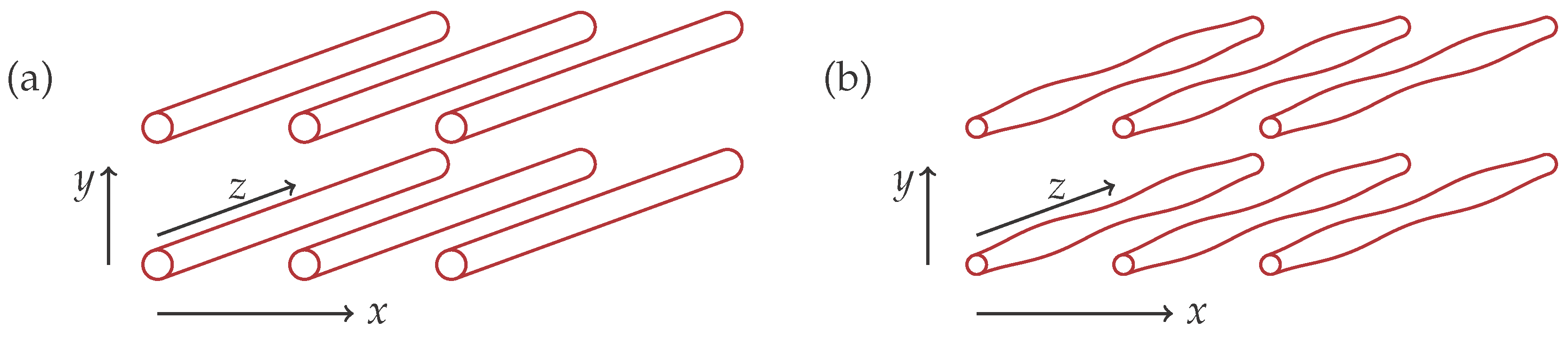
Figure 2.
In our proposed experimental system, the wire medium will not be in free space but will be confined by metallic walls. Here we represent this in two ways, each containing a finite array of wires with varying radii. First, we confine the array in a rectangular waveguide with metal side-walls (in blue-gray), and use periodic boundary conditions to treat wires of infinite length. Second, we add metallic end-walls (grey) perpendicular to the wires to change the waveguide into a closed box or cavity. In either case we can do our numerical computations for only one period of variation in the wire radii. It is very important to note that this variation only corresponds to half a period of the electric field.
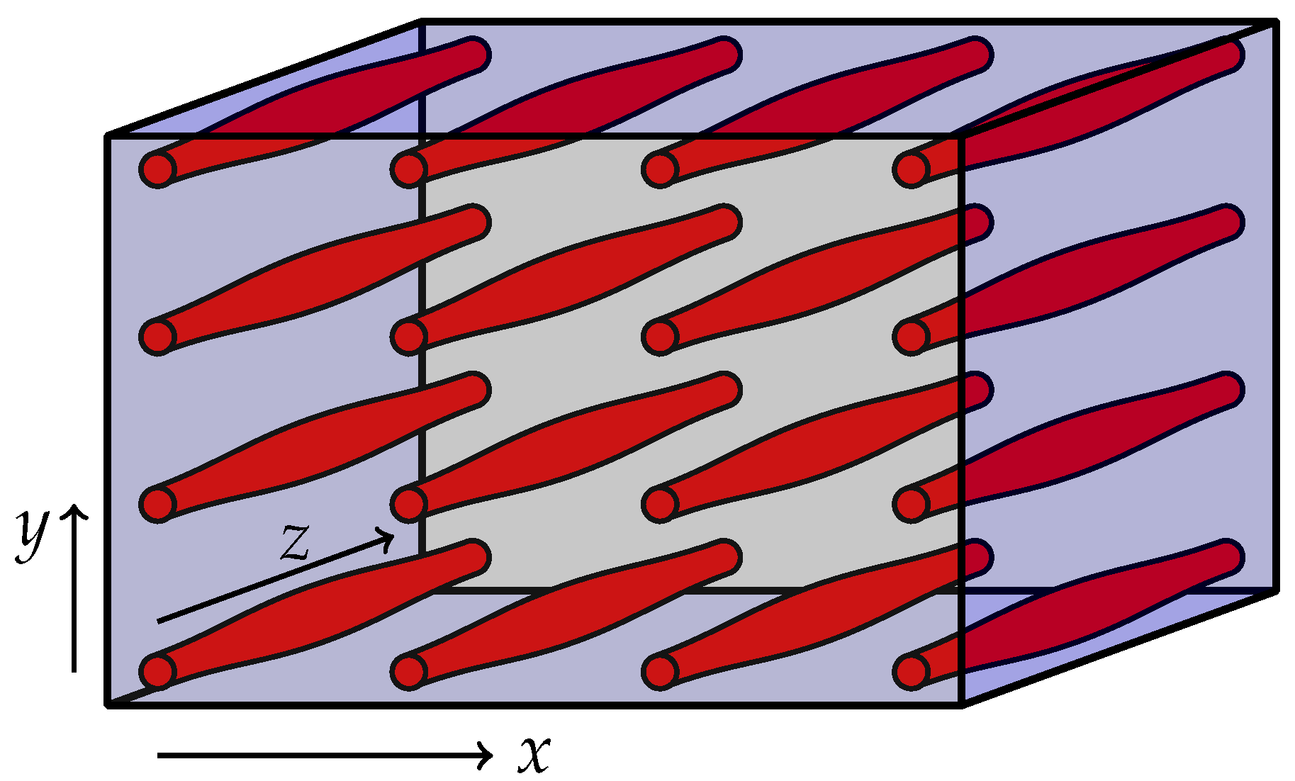
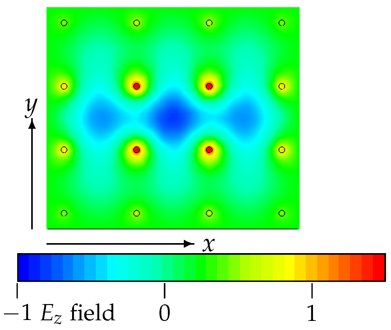
Figure 3.
Numerical results showing a longitudinal mode in a infinite array of uniform infinitely long wires; as depicted in Figure 1a. The distances between the wires are given by and . The single period of the longitudinal electromagnetic wave is given by . We show a vector plot the electric field in the plane (a) cut through the wires and (b) cut between the wires. In (c) we show the longitudinal component of the field in the plane. Observe there is a region about the wire, roughly circular in shape, where this longitudinal component is approximately zero.
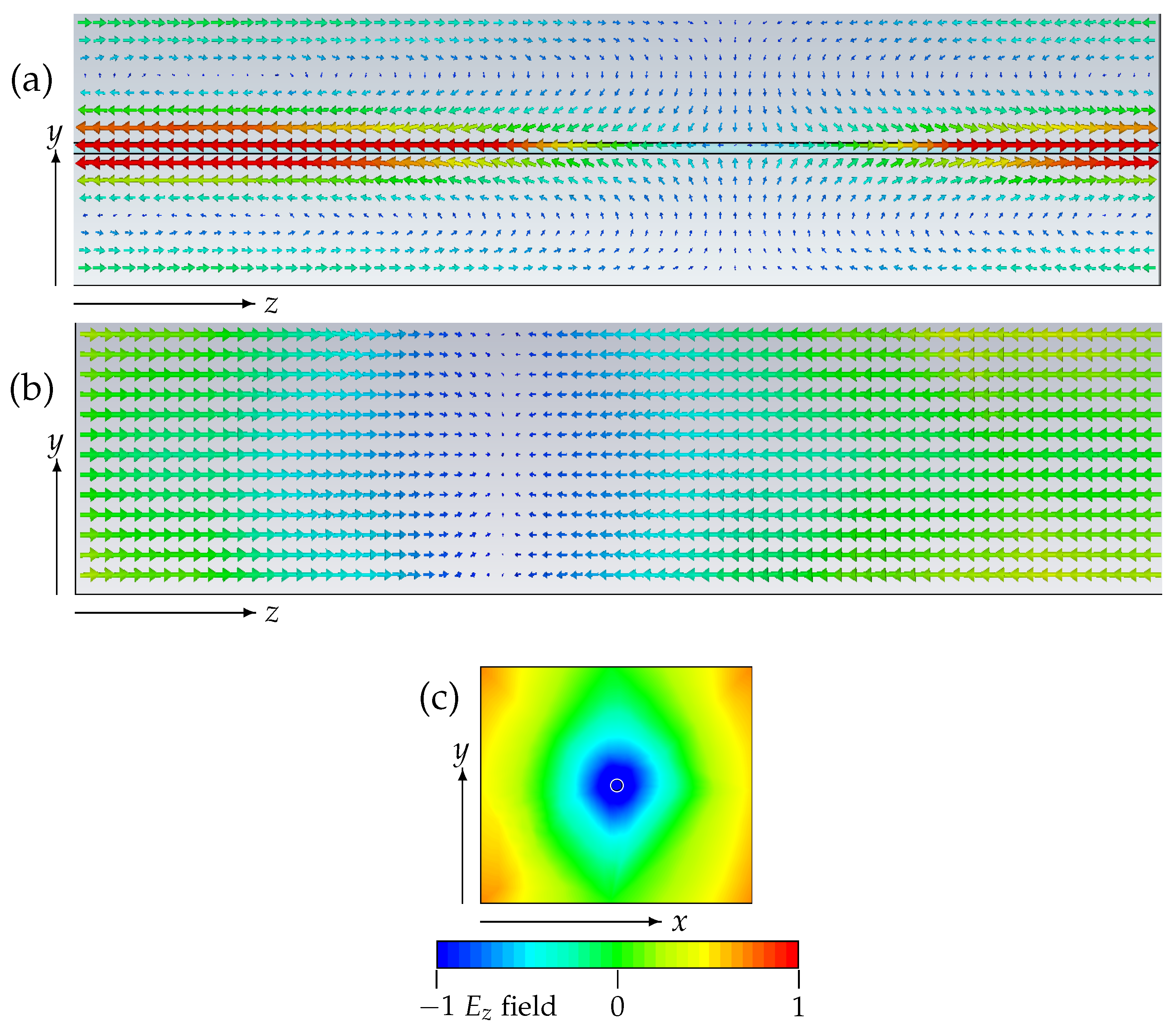
Figure 4.
How the radius of the wire affects the distance from the wire at which the longitudinal field passes through zero. This result was calculated using periodic boundary conditions for an infinite rectangular array of uniform and infinitely long wires.
Figure 4.
How the radius of the wire affects the distance from the wire at which the longitudinal field passes through zero. This result was calculated using periodic boundary conditions for an infinite rectangular array of uniform and infinitely long wires.

Figure 5.
Longitudinal component on the plane cutting across a array of uniform infinitely long wires in a waveguide. The distances between the wires are given by and . The dimensions of the waveguide are given by and . Thus, the distances of the wires closest to the waveguide walls and the walls are and . This is the data for our preferred longitudinal mode, which is only one of many.

Figure 6.
To design the required radius modulation, we need to know the variation of the effective plasma frequency of our wire array in a waveguide, as a function of wire radius, which for our chosen parameters is shown here. This data is fitted with the exponential function , where , and .
Figure 6.
To design the required radius modulation, we need to know the variation of the effective plasma frequency of our wire array in a waveguide, as a function of wire radius, which for our chosen parameters is shown here. This data is fitted with the exponential function , where , and .

Figure 7.
By combining our desired field profile (the Mathieu function of (1)) with the plasma frequency response in Figure 6 we can predict the necessary radius variation for our wire array in a waveguide. The result is shown here, with a radius that changes by about % around its average value.
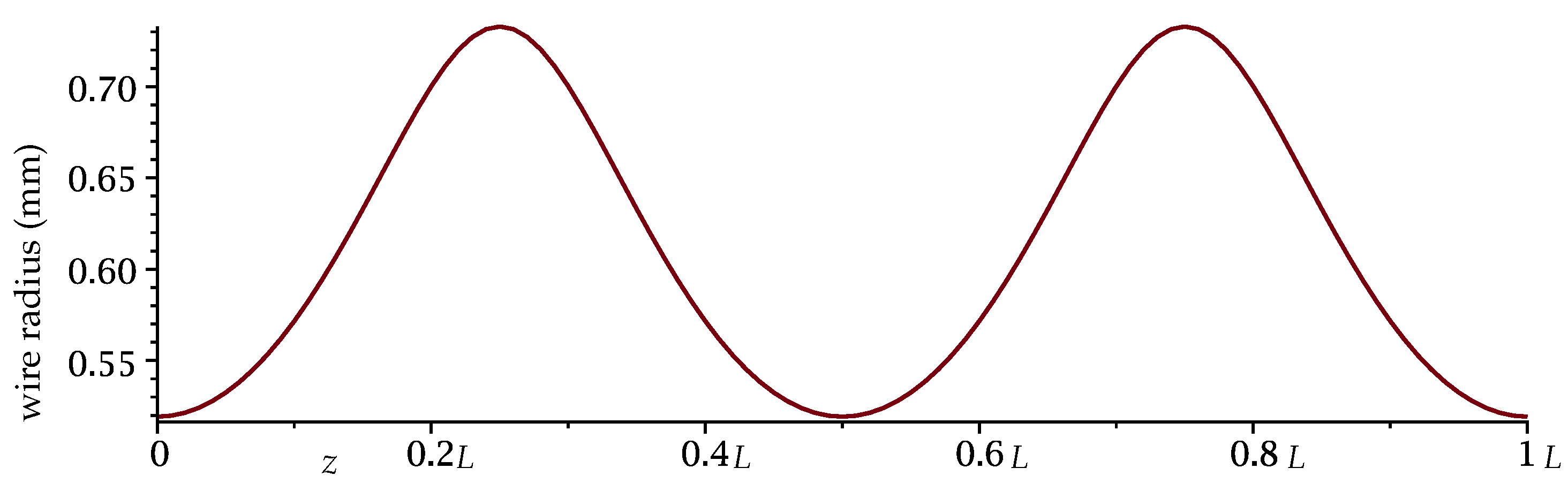
Figure 8.
The field variation in our chosen longitudinal mode as present in a array of infinitely long wires of varying radii in a waveguide. The distances between the wires are given by and . The single period of the longitudinal electromagnetic wave is given by . The dimensions of the waveguide are given by and . Thus, the distance of the wires closest to the waveguide walls and the walls are and . The electric field is shown as a vector on the plane as (a) cut through the wires, and (b) cut between the wires. In (c), the longitudinal component is shown on the . This plane is cut through the point .
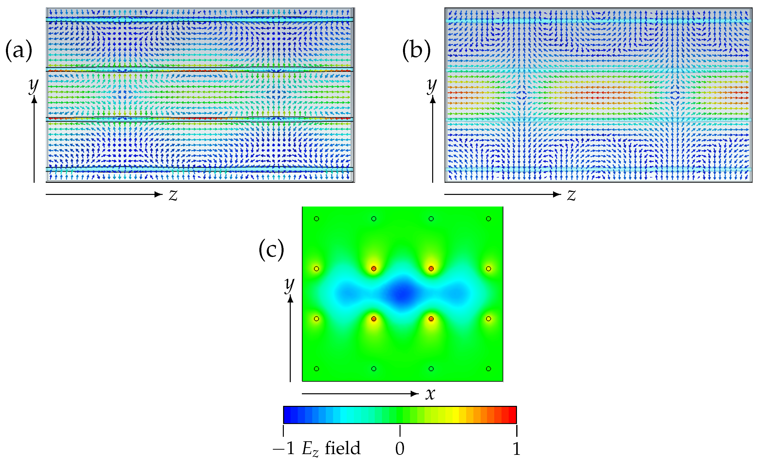
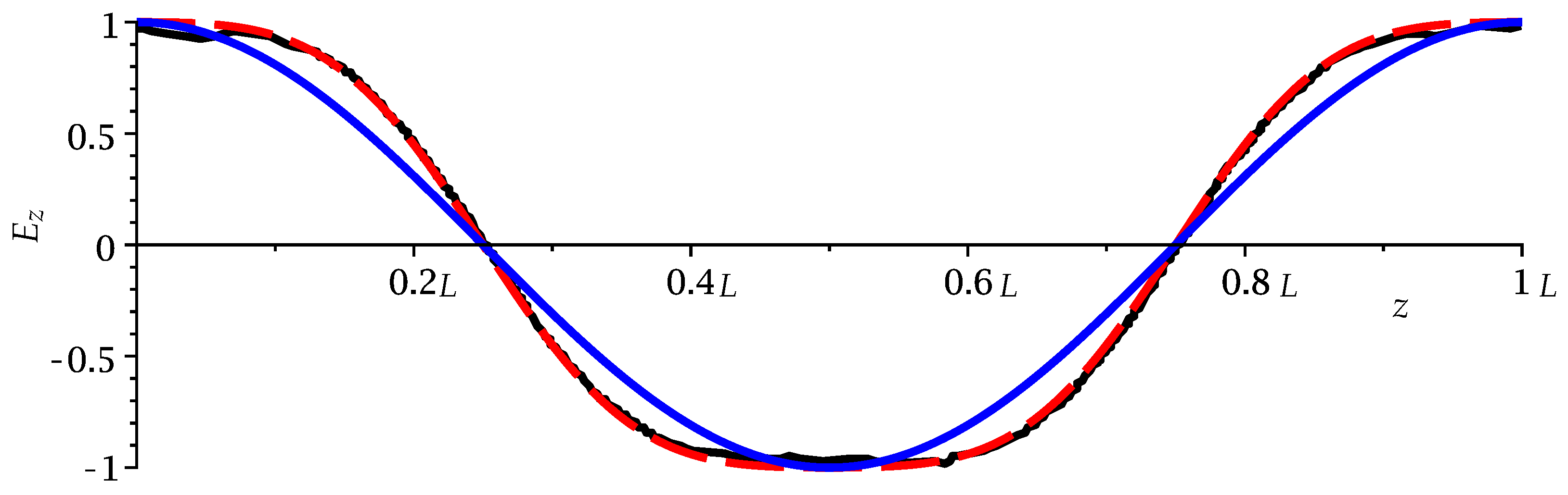
Figure 9.
Field profile shaping in a metallic waveguide containing a array of infinitely long wires of varying radii and with . The simulated field profile itself is normalised and shown with solid black lines, and is compared with the ideal Mathieu function profile shown as a dashed red curve, with a sinusoid shown in blue as a reference. In the simulation, CST gave the maximum longitudinal field as .

Figure 10.
The field variation in our chosen longitudinal mode as present in a array of wires with varying radii inside a metallic cavity, as depicted in Figure 2. The distances between the wires are given by and . The dimensions of the cavity are given by , and . Thus, the distances of the wires closest to the waveguide walls and the walls are and . The electric field is shown as a vector on the plane as (a) cut through the wires, and (b) cut between the wires. In (c), the longitudinal component is shown on the . This plane is cut through the point .

Figure 11.
Field profile shaping in a metallic waveguide containing a array of wires with varying radii in a metallic cavity, and with . The simulated field profile itself is normalised and shown with solid black lines, and is compared with the ideal Mathieu function profile shown as a dashed red curve.
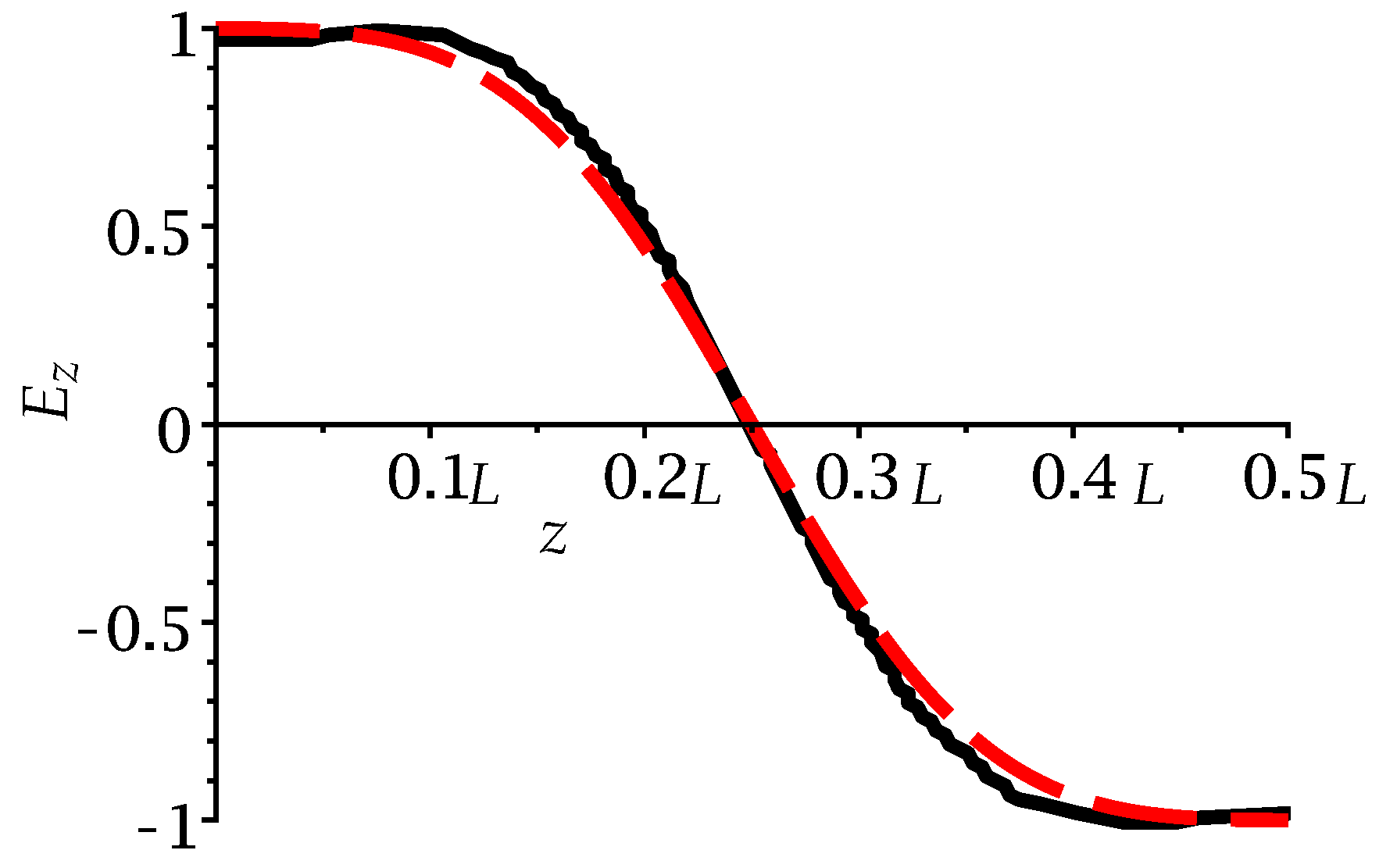
Figure 12.
Field variation of a longitudinal modes in a array of uniform infinitely long wires in a waveguide. The distances between the wires are given by and . The single period of the longitudinal electromagnetic wave is given by . The dimensions of the waveguide are given by and . Thus, the distances of the wires closest to the waveguide walls and the walls are and . Here the longitudinal component in the plane is shown.
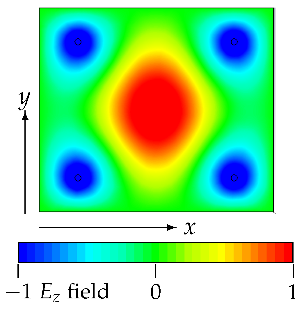
Figure 13.
Profile of component for a waveguide with infinitely long wires of varying radii (solid Black) in comparison with Mathieu function (dashed red) and sin function (blue). Here . Both and the Mathieu function are normalised. However CST gave the maximum longitudinal field as .
Figure 13.
Profile of component for a waveguide with infinitely long wires of varying radii (solid Black) in comparison with Mathieu function (dashed red) and sin function (blue). Here . Both and the Mathieu function are normalised. However CST gave the maximum longitudinal field as .
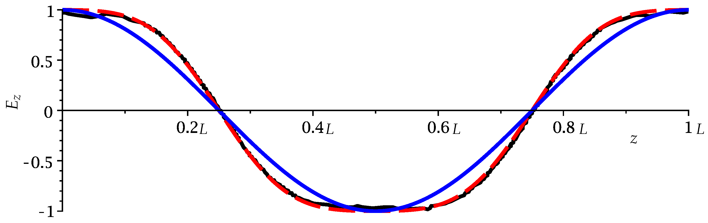
Figure 14.
An example showing the electric field vectors on a slice in the plane perpendicular to the wires. Most of the field modes near our desired longitudinal modes are of this transverse type, and should not be excited by a carefully designed (longitudinal) excitation field. The dimensions of the waveguide are the same as in Figure 8.

Table 1.
Modes of the modulated wire media in a cavity that are nearby to our chosen longitudinal mode (index 90, shown in bold). They are categorized into either transverse (‘Trans’) or longitudinal modes (‘Long’). This depends on the field patern of the electric field. The electric field in the longitudinal modes is principally parallel to the wires as in Figure 8 whereas in the transverse modes it is perpendicular to the wires, Figure 14.
| Mode Number | 82 | 83 | 84 | 85 | 86 | 87 | 88 | 89 | 90 | |
| Freq (GHz) | 12.088 | 12.098 | 12.158 | 12.159 | 12.175 | 12.250 | 12.274 | 12.388 | 12.430 | |
| Type | Long | Long | Long | Trans | Long | Trans | Trans | Trans | Our Mode | |
| Mode Number | 91 | 92 | 93 | 94 | 95 | 96 | 97 | 98 | 99 | |
| Freq (GHz) | 12.433 | 12.460 | 12.539 | 12.556 | 12.565 | 12.577 | 12.583 | 12.723 | 12.831 | |
| Type | Trans | Trans | Long | Long | Long | Long | Trans | Long | Trans | |
© 2018 by the authors. Licensee MDPI, Basel, Switzerland. This article is an open access article distributed under the terms and conditions of the Creative Commons Attribution (CC BY) license (http://creativecommons.org/licenses/by/4.0/).
Share and Cite
MDPI and ACS Style
Boyd, T.; Gratus, J.; Kinsler, P.; Letizia, R.; Seviour, R. Mode Profile Shaping in Wire Media: Towards An Experimental Verification. Appl. Sci. 2018, 8, 1276. https://doi.org/10.3390/app8081276
AMA Style
Boyd T, Gratus J, Kinsler P, Letizia R, Seviour R. Mode Profile Shaping in Wire Media: Towards An Experimental Verification. Applied Sciences. 2018; 8(8):1276. https://doi.org/10.3390/app8081276
Chicago/Turabian StyleBoyd, Taylor, Jonathan Gratus, Paul Kinsler, Rosa Letizia, and Rebecca Seviour. 2018. "Mode Profile Shaping in Wire Media: Towards An Experimental Verification" Applied Sciences 8, no. 8: 1276. https://doi.org/10.3390/app8081276
Note that from the first issue of 2016, this journal uses article numbers instead of page numbers. See further details here.