Nonlinearity Analysis and Multi-Model Modeling of an MEA-Based Post-Combustion CO₂ Capture Process for Advanced Control Design

Abstract

The monoethanolamine (MEA)-based post-combustion CO₂ capture plant must operate flexibly under the variation of the power plant load and the desired CO₂ capture rate. However, in the presence of process nonlinearity, conventional linear control strategy cannot achieve the best performance under a wide operation range. Considering this problem, this paper systematically studies the multi-model modeling of the MEA-based CO₂ capture process for the purpose of (1) implementing well-developed linear control techniques to the design of an advanced controller and (2) achieving a wide-range flexible operation of the CO₂ capture process. The local linear models of the CO₂ capture process are firstly established at given operating points using the method of subspace identification. Then the nonlinearity distribution at different loads of an upstream power plant and different CO₂ capture rates is investigated via the gap metric. Finally, based on the nonlinearity investigation results, the suitable linear models are selected and combined together to form the multi-model system. The proposed model is validated using the measurement data, which is generated from a post-combustion CO₂ capture model developed in the go-carbon capture and storage (gCCS) simulation platform. As the proposed multi-linear model has a simple mathematical expression and high prediction accuracy, it can be directly employed as the control model of a practical advanced control strategy to achieve a wide operating range control of the CO₂ capture process.

1. Introduction

One of the major contributions to CO₂ emissions is the flue gas from coal-fired power plants, accounting for over one third of total carbon emissions [1]. In recent years, monoethanolamine (MEA)-based post-combustion CO₂ capture technology has been extensively studied to capture the CO₂ from the coal-fired power plants [2,3,4,5,6,7,8,9,10,11,12,13,14,15,16]. The MEA-based CO₂ capture technique has several distinguishing features, such as a high CO₂ capture level, easy integration to power plants without much reformation of the existing plants, and relatively low construction cost, which makes it the most promising technique for commercial use [1,17]. However, the major limitation of this technology for large-scale implementation is that the solvent regeneration consumes a large amount of energy and thus significantly reduces the efficiency of the power plant [18]. Therefore, in practice, the capture plant must change the capture rate flexibly to achieve a trade-off between the electrical power supply and environmental protection [19]. For instance, the CO₂ capture rate should be reduced rapidly during the peak time of electricity consumption, when the cost of a high CO₂ capture rate overruns its benefits [20]. Moreover, as the power plant participates in the grid’s frequency regulation, the mass flow rate of flue gas can have large fluctuations, which may have a strong influence on the operation of MEA-based CO₂ capture plant. From this point of view, the CO₂ capture process must be able to adapt flexibly to the load variation of the upstream power plant.

To achieve a flexible operation of the MEA-based post-combustion CO₂ capture plant, an effective control strategy should be applied to handle the process nonlinearity, the large inertia, and the coupling effect between multiple control loops. Under the conventional design framework, the modeling of the process is the most important premise for the design of control systems. In early research works, the first principle model of the MEA-based CO₂ capture process was extensively studied, featuring the rate-based model [2,5,7,15,16,21,22,23,24,25,26] and the equilibrium-based model. In reference [2], a rate-based dynamic model of the whole CO₂ capture plant was established in gPROMS^® platform (Process System Enterprise, London, UK) and validated using experimental data. In reference [13], the model of an absorber column was developed, and several modeling approaches for the reactive absorption were compared. In reference [25], the dynamic model of the absorber for a laboratory-scale pilot plant was constructed in an Aspen Plus^® simulator (AspenTech, Bedford, MA, USA). Some configuration and operation parameters, such as the packing height of the absorber, the ammonia concentration of lean solution, and the CO₂ loading of lean solution, were optimized. In references [22,27,28], rate-based models were compared with equilibrium-based models and showed better accuracy than the equilibrium-based models. As the first principle model can provide high-accuracy predictions of the full operating range of the real process, it was employed as a simulation platform to investigate the dynamic characteristics of the CO₂ capture process and validate the performance of designed control strategies. However, the complexity of the first principle model makes it difficult to be utilized for the controller design. On the one hand, the construction of the first principle model requires massive knowledge of the process, such as the principle of the chemical reactions, thermodynamics, and specifications of the capture plant. On the other hand, because the first principle model consists of numerous nonlinear differential equations which are difficult to solve, implementing the first principle model in control design is time-consuming and weak in robustness [29].

To address this problem, data-driven modeling approaches were studied to develop the black-box model of the MEA-based CO₂ capture process. Although black-box models are generally less accurate than the first principle model, they have much simpler mathematical expression and thus can be more easily employed for the derivation of control algorithms. The conventional black-box models in the CO₂ capture process for control system design are linear models [4,5,6,17,19,30]. In reference [30], the continuous transfer function model of the CO₂ capture process was identified at the selected operating point. In reference [19], the discrete first-order transfer function models were derived for the control of the reboiler pressure, the reboiler temperature, and CO₂ capture rate. In references [4,6,17], the linear state-space model was established for the model predictive control of the CO₂ capture process. However, as the MEA-based CO₂ capture plant has to operate flexibly under a wide operating range, the resulting process nonlinearity will render the linear models inaccurate. Consequently, the controllers developed based on these models may have severe performance degradation when the operating point of the capture process deviates far from the designed points.

Considering the limitations of the linear model, nonlinear models were proposed to describe the full operating range dynamics of the CO₂ capture process. In reference [31], the artificial neural network (ANN) with multilayer feed-forward form was developed to capture the nonlinear relationship of the inputs and outputs for the MEA-based post-combustion CO₂ capture process, which covered the entire actual operating range of the plant. The training data of the ANN model was generated from the first principle model built up using the process simulator CO2SIM (SINTEF, Trondheim, Norway). In reference [32], a bootstrap aggregated neural network (BANN) was trained to establish the relationship between the CO₂ capture rate and several process variables, including the mass flow rate and CO₂ concentration of the inlet flue gas, temperature and MEA concentration of the lean solvent. The BANN model showed better prediction performance than the conventional ANN model. In reference [33], multiple extreme learning machines (ELM) were proposed to predict the CO₂ capture rate given a set of process inputs. The multiple ELMs had relatively fast learning speed and enhanced prediction reliability in comparison with the single ELM. In reference [14], a 4 × 3 multivariable nonlinear autoregressive (NLARX) model for the CO₂ capture process was developed and validated using experimental data. The NLARX model was then employed for controllability analysis and control system design. Although compared with linear models the nonlinear models are more accurate for a wide operation range of the CO₂ capture process, it takes much more effort to determine the model structure and identify the model parameters. For instance, the number of hidden layers and nodes in the ANN model should be carefully chosen to avoid the overfitting of the training data. Furthermore, the control strategies based on such nonlinear models are mostly not applied in practice, as the mathematical problems extracted from the control algorithm are generally difficult to solve.

To overcome these issues and develop a model suited for advanced CO₂ capture control design, this paper studies the multi-model modeling approach for the MEA-based post-combustion CO₂ capture process. The basic idea of multi-model modeling is to combine several linear models at different operating points to approximate the nonlinear dynamics of the process.

A qualified multi-linear model for control design should meet the following requirements:

(1)

Good prediction accuracy and concise model structure. In general, increasing the number of the local linear models will improve the model accuracy; however, it also intensifies the complexity of the model structure, which can lead to a significant growth in the computation time of the model predictions and thus make the multi-linear model lose its advantage. Therefore, the accuracy and complexity of the multi-linear model must be balanced by choosing appropriate local linear models. In order to determine the best local linear models for the construction of a multi-linear model, the nonlinearity distribution of the process must be investigated.

(2)

Proper mathematical expression. For multi-input multi-output (MIMO) nonlinear process, the model with an appropriate mathematical expression can greatly reduce the complexity of the advanced controller design and the computational cost of the control law.

Considering these requirements for multi-model system development and the flexible operation of the CO₂ capture plant, this paper investigates the nonlinearity distribution of the process to select proper local linear models and studies the construction of the multi-linear model. The local linear models at different CO₂ capture rates and flue gas mass flow rates are firstly obtained via a subspace identification approach such that the model with the state-space form can be directly obtained, which facilitates the derivation of advanced controllers. Then the nonlinearity distribution of the process is analyzed using the gap metric as the tool for quantifying the magnitude of the process nonlinearity [34,35]. As mentioned above, the CO₂ capture plant should operate flexibly under large variations of the flue gas and CO₂ capture rate. Thus, in this study the process nonlinearity distribution is analyzed for these two operating situations. Finally, based on the nonlinearity distribution, the identified linear state-space models are combined to construct the multi-linear model. As the proposed multi-linear model has a mathematical expression similar to the linear model, the linear control techniques can be modified to handle the nonlinearity of the CO₂ capture process.

This work has two major contributions: (1) the nonlinearity distribution of the MEA-based post-combustion CO₂ capture process is systematically investigated using the gap metric; (2) a multi-linear model of the CO₂ capture process is developed, which can provide a foundation for the advanced control system design.

The main content of this paper is organized as follows: Section 2 presents the dynamic model of the MEA-based post-combustion CO₂ capture plant model developed using the go-carbon capture and storage (gCCS) toolkit. Section 3 explores the nonlinearity distribution of the CO₂ capture process and establishes the multi-linear model. Section 4 presents the simulation results. Section 5 introduces the proposed multi-linear model for advanced control system design. Section 6 summarizes the results and draws the conclusions.

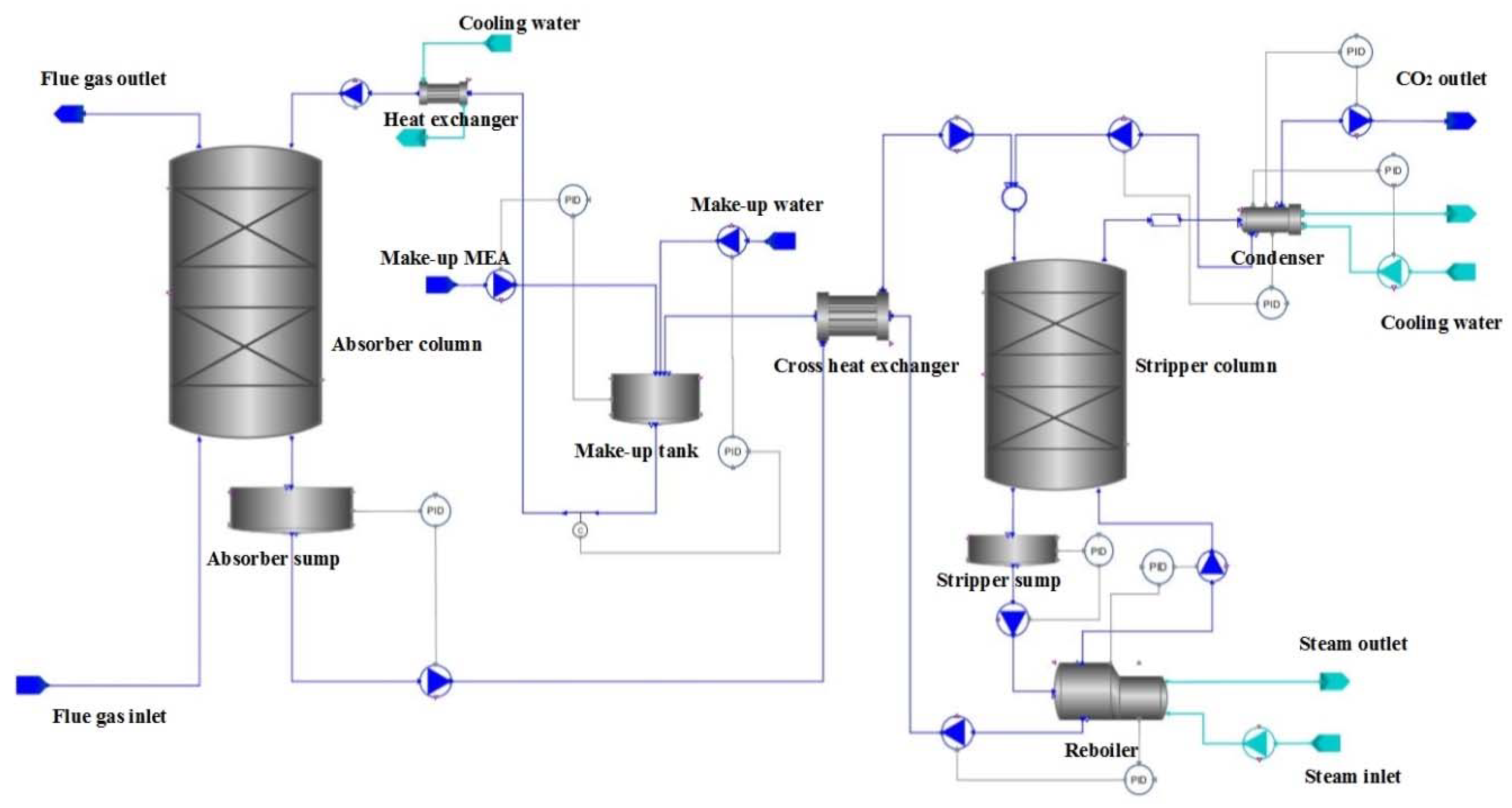
2. Dynamic Model Configuration for the CO₂ Capture Process

This section presents the dynamic model of an MEA-based post-combustion CO₂ capture plant for a 1 MWe power plant, which is used as the simulation platform in this study. All of the process modules are developed using the gCCS toolkit, which can provide high-fidelity models for the MEA-based CO₂ capture process. The gCCS, developed by the process systems enterprise (PSE, London, UK) company, is professional software used in studying the dynamics of amine-based post-combustion CO₂ capture processes [36]. The process topology in gCCS is presented in Figure 1, which describes the major processes within the MEA-based post-combustion CO₂ capture system.

Before decarbonization, the flue gas from the power plant is firstly desulphurized and denitrified. The treated flue gas is then cooled to 305–315 K before entering the bottom of the absorber. The flue gas and lean MEA are introduced counter currently into the absorber such that the CO₂ can be sufficiently removed. After that the flue gas, mainly consisting of water and nitrogen, is emitted to the atmosphere, and the lean MEA becomes rich MEA.

After the absorption reaction in the absorber, the rich solvent is further heated in a cross-heat exchanger by the hot lean MEA from the reboiler. Thereafter, the rich MEA enters the stripper and releases a part of the captured CO₂. In the stripper, the energy required for releasing the CO₂ is provided by the high temperature gas from the reboiler. Finally the rich MEA is sent to the reboiler and heated up to 380–390 K by the steam extracted at the crossover pipe between the intermediate and low pressure steam turbine in the power plant [15]. In this way, the remaining captured CO₂ is released. The released gas from stripper is condensed in the condenser to obtain pure CO₂ gas.

The CO₂ capture plant in this paper is designed for a 1 MWe coal fired power plant, which can generate as much as 0.13 kg/s flue gas with 25.2 wt % CO₂ content at the 100% load condition. The established capture plant model is valid when the power plant operates between 40% and 100% load. The gCCS models of absorber and stripper column are developed based on the two-film theory, while the reboiler and the condenser models are developed using the lumped parameters approach.

In the gCCS models, the following assumptions are made:

(1)

All the chemical reactions are in equilibrium state.

(2)

The pressure drop along the column is linear.

(3)

The holdup in the vapor balk and the solvent degradation are neglected.

(4)

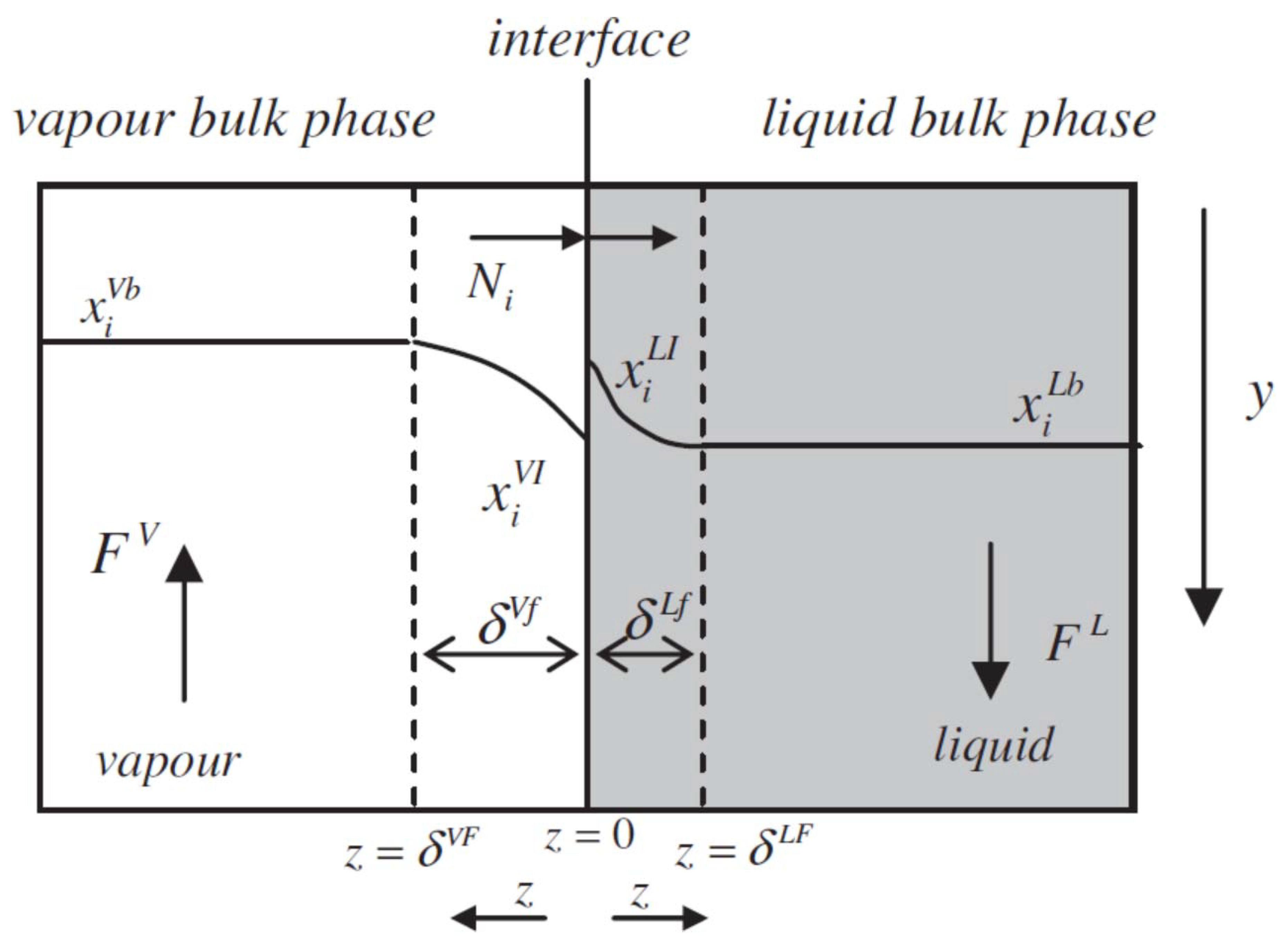
The phase at the interface between liquid and vapor films attains equilibrium.

The bulks, films, and interface of liquid and vapor in the packed columns are shown in Figure 2. The key dynamic equations of the packed column are presented as follows.

The mass and energy balance of the liquid bulk can be described using differential equations [2]:

$$\frac{d{M}_i}{dt}=\frac{-1}{L·A}\frac{\partial F_i^L}{\partial y}+N_i·Sp·\omega ·M{W}_i$$

(1)

$$\frac{dU}{dt}=\frac{-1}{L·A}\frac{\partial F_H^L}{\partial y}+Sp·\omega ·\left(H_{liq}^{cond}+H_{liq}^{conv}+H_{abs}\right)+HL$$

(2)

where M_i is the i-th component hold up, L and A are the length and cross-sectional area of column section, $F_i^L$ is the liquid component mass flow along the axis of the column, N_i is the molar flux to and from the liquid bulk, MW_i is the molecular weight, Sp is specific area, ω is the wetted area ratio, U is the energy hold up, $F_H^L$ is the energy flow along the axis of column, $H_{liq}^{cond}$, $H_{liq}^{conv}$, and $H_{abs}$ are the heat fluxes of liquid conduction, convection, and chemical reactions at the liquid film-liquid bulk interface, respectively, and HL is the heat loss to the environment.

Similarly, the mass and energy balance of the vapor bulk can be modeled as [2]:

$$0=\frac{-1}{L·A}\frac{\partial F_i^V}{\partial y}-N_i·Sp·\omega ·M{W}_i$$

(3)

$$0=\frac{-1}{L·A}\frac{\partial F_H^V}{\partial y}+Sp·\omega \left(H_{vap}^{cond}+H_{vap}^{conv}\right)$$

(4)

where $F_i^V$ is the vapor component mass flow along the axis of the column, and $H_{vap}^{cond}$ and $H_{vap}^{conv}$ are the heat fluxes of vapor conduction and convection at the vapor film-vapor bulk interface, respectively.

The mass transfer rates in the vapor and liquid films can be determined using the Maxwell-Stefan Formulation:

$$\frac{1}{\delta }\frac{\partial x_i^M}{\partial z}=\frac{1}{c_t}{\displaystyle \sum }_{k=1}^{nc}\left(\frac{x_i^M{N}_k-x_k^M{N}_i}{{\chi }_{i,k}}\frac{{\mu }^R}{\mu }\frac{T}{298.15}\right), k\ne i$$

(5)

where δ is the film thickness, $x_i^M$ is the molar fraction of the i-th component, c_t is the total molar concentration, nc is the number of components, χ_i,k is the diffusivity, μ and μ^R are the viscosity and reference viscosity, respectively, and T is the temperature.

The interface model is formulated as:

$$f_i^L{x}_i^{M,L}=f_i^V{x}_i^{M,V}$$

(6)

where $f_i^L$ and $f_i^V$ are the liquid and vapor fugacity coefficients, and $x_i^{M,L}$ and $x_i^{M,V}$ are the equilibrium molar components in the vapor and liquid phases.

The overall reaction for carbonate formation can be given as [37]:

$$C{O}_2+MEA+B\rightleftharpoons MEACO{O}^{-}+B{H}^{+}$$

(7)

The reaction rate of CO₂ can be calculated as [37]:

$$r_{C{O}_2}=\left\{k_{MEA}^T\left[MEA\right]+k_{H_{2}O}^T\left[H_{2}O\right]\right\}\left[MEA\right]\left[C{O}_2\right]-\left(\frac{k_f^T}{K_{eq}^T}\right)\left[MEA{H}^{+}\right]\left[MEACO{O}^{-}\right]$$

(8)

where B = MEA and/or H₂O, $k_{MEA}^T$ and $k_{H_{2}O}^T$ are the third order kinetic rate constant of MEA and H₂O, respectively, $k_f^T$ is the forward reaction rate, $k_{eq}^T$ is the equilibrium constant, and the superscript T represents the temperature dependence.

The physical properties of the solvents in the capture process are calculated using the go-statistical associating fluid theory (gSAFT) package (Process System Enterprise, London, UK), which is also developed by the PSE Company based on the Statistical Association Fluid Theory [38]. The steady-state process conditions of the nominal working point, that is 100% power plant load and 80% CO₂ capture rate, are shown in

Table 1. Steady-state process conditions of the nominal operating point. ID: identification.

Stream ID	Temperature (K)	Mass Flow (kg/s)	Mass Fraction
			H2O	CO2	MEA	N2
Lean MEA to Absorber	313.9	0.777	0.618	0.074	0.308	0.000
Rich MEA from Absorber	323.9	0.798	0.593	0.104	0.303	0.000
Inlet Flue Gas	314.3	0.130	0.015	0.252	0.000	0.733
Outlet Flue Gas	317.5	0.108	0.060	0.060	0.000	0.879

, based on reference [13].

Within the CO₂ capture system, there are many process variables which should be well controlled, such as the liquid level of the absorber sump, the reboiler pressure, etc. Among these variables, the control of the CO₂ capture rate and reboiler temperature are of the highest importance because the CO₂ emission level must be controlled to satisfy the environmental demand and the temperature in the reboiler should be maintained to keep the balance between energy supply and consumption. The lean solvent flow rate and extracted steam flow rate have the most significant influence on the two key controlled variables, as demonstrated in references [3,7,12,30,39]. For these reasons, the dynamic relationship between these four key variables is studied in this paper, which results in a 2 × 2 model structure for the nonlinearity analysis and the construction of the multi-linear model. The other process variables are controlled to the given set point by well-tuned decentralized proportional integral (PI) controllers, and hence the control of these variables is not considered in the advanced control structure. The entire control structure of the CO₂ capture process is presented in Figure 3.

The transfer function of the PI controller is defined as:

$$\frac{u\left(s\right)}{e\left(s\right)}=K_p\left(1+\frac{K_I}{s}\right)$$

(9)

where K_p is the proportional coefficient and K_I is the integral coefficient. The PI controllers are tuned using the conventional Ziegler-Nicholas methods [40], in which the proportional and integral gain are calculated based on empirical formulas. The configurations of the PI controllers are listed in

Table 2. Set points and tuning parameters of the decentralized PI. K_p: proportional coefficient, K_I: integral coefficient.

Controlled Variable	Manipulated Variable	Set Point Value	Kp	KI
Absorber sump liquid level	Absorber sump outlet liquid mass flow	1.25 m	200	0.10
Stripper sump liquid level	Stripper sump outlet liquid mass flow	1.25 m	200	0.10
Condenser temperature	Cooling water mass flow	313.15 K	80	0.06
Condenser pressure	Condenser outlet gas mass flow	1.69 × 105 Pa	5.5	0.15
Condenser liquid level	Condenser outlet liquid mass flow	0.25 m	100	0.10
Reboiler pressure	Reboiler outlet gas mass flow	1.79 × 105 Pa	5.0	0.15
Reboiler liquid level	Reboiler outlet liquid mass flow	0.25 m	100	0.10
Make-up tank liquid level	Tank outlet liquid mass flow	1 m	20	0.10
Mass fraction of MEA	Make-up MEA mass flow	0.307	10	0.05

.

3. Multi-Model Modeling of the CO₂ Capture Process

In this section, the multi-model modeling approach is studied for the CO₂ capture process. The local linear models at typical operating points are firstly identified via the subspace identification approach. Then the gap metric of the local linear models is calculated to investigate the distribution of the process nonlinearity. In the end, based on the nonlinearity distribution, the multi-linear model is constructed from the selected local linear models.

3.1. Identification of the Local Linear Models

As mentioned above, the flexible operation requires the CO₂ capture system to adapt quickly to the variation of flue gas and the CO₂ capture rate demand. Therefore, the local linear models are identified at different CO₂ capture rates (Group I) and different mass flows of flue gas (Group II), covering the major operating range of the CO₂ capture process. In Group I, the load of the power plant is fixed to 100% load, which can generate 0.13 kg flue gas per second, and the CO₂ capture rate varies from 50% to 95%. In Group II, the CO₂ capture rate is fixed to 80%, while the flue gas changes from 0.13 kg/s to 0.07 kg/s. The selected operating points in Group I and Group II for nonlinearity analysis are listed in

Table 3. Selected operating points.

Groups	CO2 Capture Rate (%)	Flue Gas Mass Flow Rate (kg/s)	Lean MEA Mass Flow Rate (kg/s)	Steam Mass Flow Rate (kg/s)	CO2 Mass Fraction in Outlet Flue Gas (kg/kg)	MEA Mass Fraction in Lean Solvent (kg/kg)
Group I	50	0.13	0.4468	0.02498	0.1350	0.3078
Group I	60	0.13	0.5572	0.03223	0.1121	0.3071
Group I	70	0.13	0.6687	0.03987	0.0873	0.3079
Group I	80	0.13	0.7765	0.04764	0.0603	0.3079
Group I	90	0.13	0.8841	0.05571	0.0314	0.3078
Group I	95	0.13	0.9428	0.06012	0.0160	0.3073
Group II	80	0.07	0.4064	0.02127	0.0602	0.3073
Group II	80	0.09	0.5257	0.03032	0.0598	0.3076
Group II	80	0.11	0.6501	0.03876	0.0603	0.3080
Group II	80	0.13	0.7765	0.04764	0.0601	0.3075

.

For each selected operating point, the subspace identification approach (SID) is employed to obtain the local linear model with a state-space form. Compared with the conventional transfer function model, because the state-space model has a simple expression for the multi-input multi-output system, it is very convenient to describe the CO₂ capture system. Moreover, the SID algorithm uses numerically efficient methods, such as QR factorization and singular value decomposition, which do not involve any nonlinear optimization techniques and thus avoids the computational issues of the conventional prediction error methods (PEM) for the identification of MIMO systems [41]. The major procedures of SID are summarized as follows:

(1)

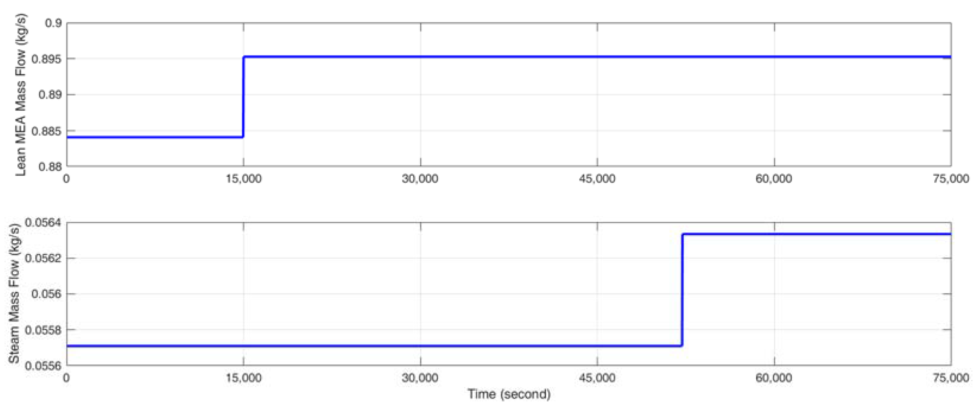
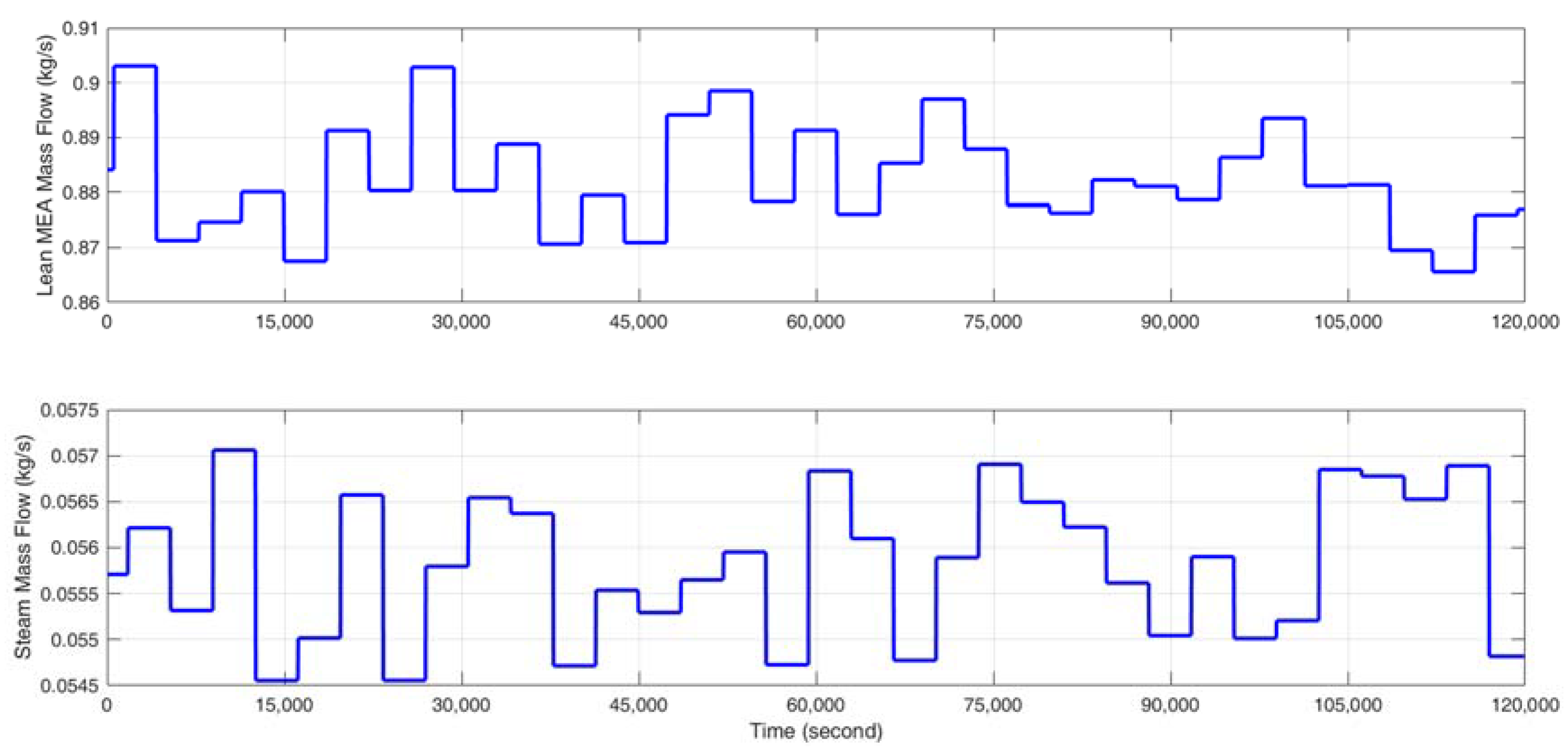
Stimulate the CO₂ capture process with a random identification signal, which fluctuates about ±2% of the steady-state input value around the selected operating point so that the CO₂ capture rate varies about ±5% in absolute value and the reboiler temperature varies within ±0.5 K. The gCCS simulator can provide data at every second; however, considering the slow dynamics of the MEA-based post-combustion CO₂ capture process, the sampling time is selected as 30 s. The input signal is designed to change every 3000 s since a fast identification signal change is not suitable for capturing the dynamics and the steady state of the CO₂ capture process.

(2)

Construct the Hankel Matrixes using the collected input-output data, and then partition the Hankel Matrixes into past and the future block matrixes.

(3)

Combine the partitioned Hankel Matrixes into a new data matrix and perform QR factorization on them.

(4)

Calculate the subspace matrix from the factorization results of step (3) and perform singular-value decomposition (SVD) on the subspace matrix. Extract the system matrixes from the subspace matrices.

More details of SID are introduced in reference [42] and not repeated here. The identified local model at the j-th operating point has the following state-space form:

$$\{\begin{array}{c}{x}_j\left(k+1\right)=A_j{x}_j\left(k\right)+B_{j}u\left(k\right)\\ y_j\left(k\right)=C_j{x}_j\left(k\right)+D_{j}u\left(k\right)\end{array}$$

(10)

where A_j, B_j, C_j, D_j are constant matrixes identified via the SID method. u and y_j are the model inputs and outputs, respectively. x_j is the state vector. k represents the present sample time. Note that, different from the transfer function methods that have to identify four models for the 2 × 2 system, the state-space model can use only one model to represent the relationship between the multiple inputs and outputs.

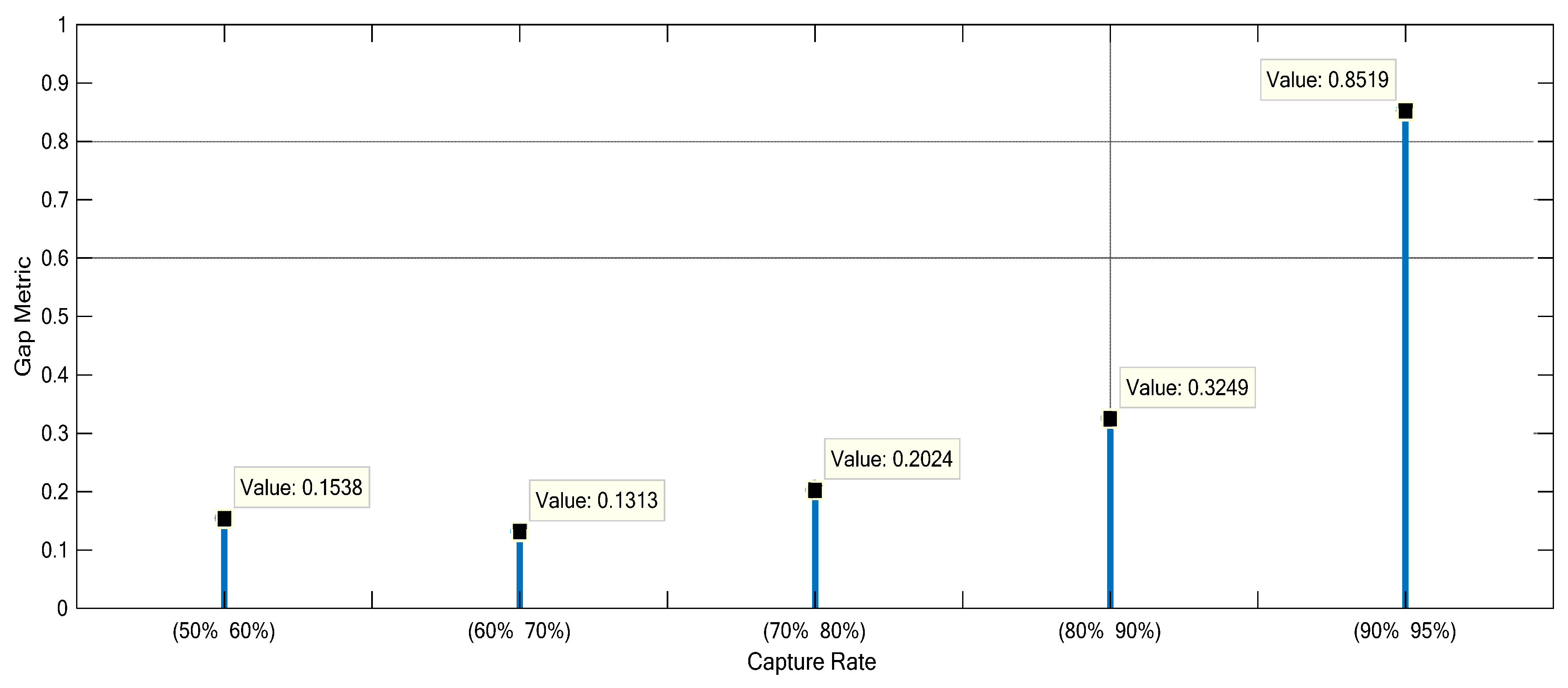
3.2. Nonlinearity Analysis of the Monoethanolamine-Based Post-Combustion CO₂ Capture Process

In this section, the nonlinearity distribution of the MEA-based post-combustion CO₂ capture process is analyzed using the gap metric. As mentioned before, the CO₂ capture plant must operate flexibly under the change of the flue gas mass flow rate and desired CO₂ capture rate; therefore, the nonlinearity distribution is analyzed for these two scenarios.

The gap metric can be regarded as the “distance” between two linear models, which is originally proposed as a tool to analyze the robust stability for closed-loop linear systems [43,44]. In later studies, the gap metric was found especially useful in the evaluation of process nonlinearity and thus it is applied in the model bank selection of multi-linear models [45,46,47].

The gap metric of two linear models is defined as follows. Denote two linear models as P₁ and P₂, and perform the normalized right coprime factorization on P₁ and P₂:

$$P_1=N_1{M}_1^{-1}$$

(11)

$$P_2=N_2{M}_2^{-1}$$

(12)

Then the gap metric between P₁ and P₂ is calculated as:

$$\delta \left(P_1,P_2\right)=max\left\{in{f}_{Q\in H_{\infty }}\parallel \left[\begin{array}{c}{M}_1\\ N_1\end{array}\right]-\left[\begin{array}{c}{M}_2\\ N_2\end{array}\right]Q{\parallel }_{\infty },in{f}_{Q\in H_{\infty }}\parallel \left[\begin{array}{c}{M}_2\\ N_2\end{array}\right]-\left[\begin{array}{c}{M}_1\\ N_1\end{array}\right]Q{\parallel }_{\infty }\right\}$$

(13)

where δ(P₁,P₂) is bounded between 0 and 1.

If the gap metric between two local linear models is close to one, it means their dynamic behavior is quite different and thus the process nonlinearity is strong between the two operating points. On the contrary, if the gap metric is close to zero, it means the dynamics of the two models are similar and the process nonlinearity is weak.

The gap metric of the neighboring local models of the CO₂ capture rate (Group I) and flue gas mass flow (Group II) are plotted in Figure 4 and Figure 5, respectively.

Figure 4 shows that there is an increasing trend in the gap metric value as the capture rate increases from 50% to 95%. The peak value of the gap metric is observed at a CO₂ capture rate of 95%; however, at other operating points the gap metric is much smaller. This indicates that the process nonlinearity is extremely strong around 95% CO₂ capture rate but relatively weak from 50% to 90%. An intuitive explanation for the strong nonlinearity at 95% CO₂ capture rate is that: as most of the CO₂ gas is already captured, it becomes much harder to extract the remaining CO₂ from the flue gas, which significantly alters the dynamic behavior of the CO₂ capture process. However, as seen in Figure 5, the operating points with different flue gas mass flow rates have small and similar gap metric values, which means the local models with different flue gas mass flows but the same CO₂ capture rate have similar dynamics. Therefore, the flue gas mass flow rate’s influence on the distribution of process nonlinearity is very small.

These results can be further explained using the first principle models of the mass balance, energy balance, and chemical reactions in the packed column. As seen in Equation (8), the reaction rate of CO₂ is directly determined by the concentration of reactants and reaction constants. Since in practice the reaction temperature is generally well controlled to the economic operating point, the temperature has little influence on the reaction constants and on the energy balance in the packed column. Hence, the reaction rate of the CO₂ mainly depends on the concentration of reactants. Generally when the load of the power plant changes, the mass flow rate of flue gas will change accordingly while the components of the flue gas, that is, the concentration of CO₂, N₂, etc., exhibit minor change [48]. In such a case, to maintain the designed 80% CO₂ capture rate, the mass flow rate of lean MEA change almost proportionally to the mass flow rate of flue gas, as seen in Table 3. Also note that the mass fraction of MEA and H₂O in the lean solvent remains unchanged owing to the make-up of water and MEA. Therefore, at the working points of different power plant loads and the same CO₂ capture rate, the inlet flow of the absorber not only has almost the same concentrations of the reactants but also the same liquid/gas (L/G) ratio. This indicates that the solutions of model equations around these working points are similar, which results in similar dynamics and weak nonlinearity. On the other hand, at the working points of same power plant load and different CO₂ capture rates, the L/G ratio undergoes a significant change, which has a great influence on the mass balance in the packed column and consequently changes the reaction rate of CO₂. At the working point with a high CO₂ capture rate, increasing the mass flow rate of lean solvent will lead to a smaller increase of the CO₂ capture rate than at the working point with a low CO₂ capture rate, because the low concentration of CO₂ gradually becomes the dominant factor of the reaction rate. Therefore, the process nonlinearity becomes increasingly strong as the CO₂ capture rate grows.

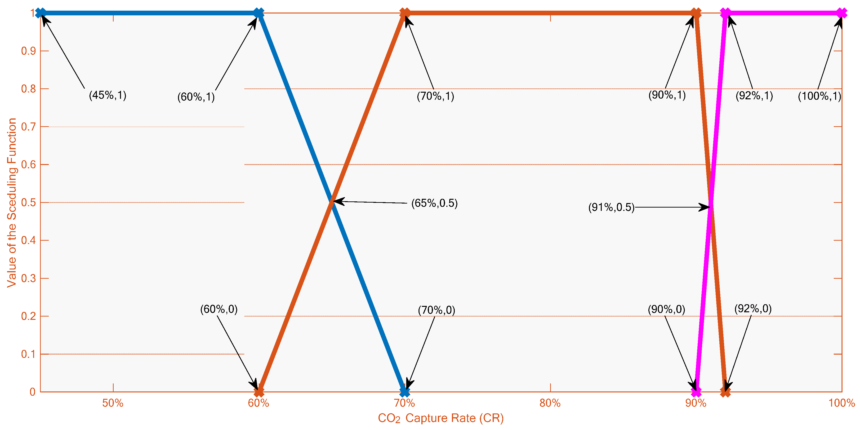
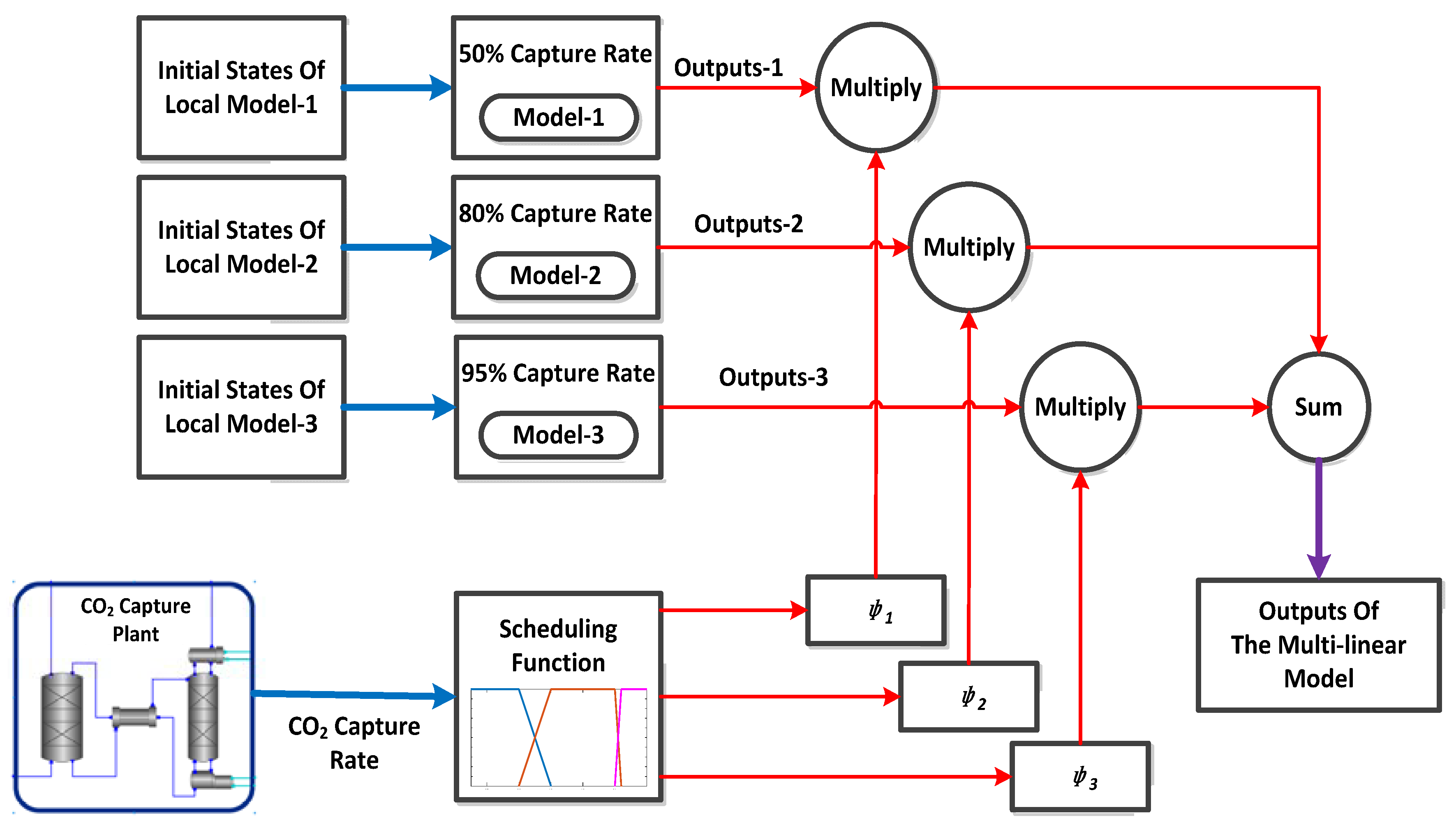
3.3. Derivation of the Multi-Linear Model

The investigation result shows that the nonlinearity of the CO₂ capture process is dependent on the CO₂ capture rate rather than the flue gas mass flow; therefore, the CO₂ capture rate was selected as the scheduling variable to select the local linear models for constructing an advanced controller. In general, to increase the accuracy of the multi-linear model, as many local linear models as possible should be used for prediction. However, this also increases the complexity of the multi-linear model and the resulting advanced controller. For instance, for multi-model model predictive control methods, the computational cost can be proportional to the number of local models. On the other hand, the effectiveness of increasing local models on improving the prediction accuracy can be minor when the process nonlinearity is weak. Hence, the number of local models in the multi-linear model should be determined according to the nonlinearity analysis such that the model complexity and accuracy can be balanced. Since the operating range from 80% to 95% CO₂ capture rate shows stronger nonlinearity than the operating range, from 50% to 80% CO₂ capture rate, the local linear model with 80% CO₂ capture rate was selected as the intermediate point for the two operating ranges. The local models with 50% and 95% CO₂ capture rate were selected to cover the full operating range.

Note that the local linear models can represent the dynamic relationship between the key controlled variables and manipulated variables around specific operating points, while they cannot describe the dynamics of the whole CO₂ capture plant. Hence, they can only be employed to construct multi-linear models for designing model-based controllers but are not suitable for simulating the whole plant. Generally, the controllers designed based on a multi-linear model will have better performance than the single-model controllers, because the multi-linear model can predict the process outputs in a more accurate manner.

Trapezoidal scheduling functions were then designed, as shown in Figure 6, to link the three local linear models together and form the integrated multi-model system. As seen in Figure 6, when CO₂ capture rate (CR) is between 45% and 60%, ψ₁ = 0 and ψ₂ = ψ₃ = 0, which denotes the dynamics of the CO₂ capture process, is described solely by the local model with 50% CR. When CR is between 60% and 70%, ψ₁ ≠ 0, ψ₂ = 1 − ψ₁, and ψ₃ = 0, which denotes the dynamics of the CO₂ capture process, is described by combining the local models with 50% CR and 80% CR. The scheduling function in the remaining operating ranges can be explained similarly.

The prediction function of the multi-linear model is derived as follows:

Suppose at time k, the initial state of the j-th local model is x_j(k). The i-step-ahead predictions of the j-th local model can be expressed as:

$$\{\begin{array}{c}{x}_j\left(k+i+1\right)=A_j{x}_j\left(k+i\right)+B_{j}u\left(k+i\right)\\ y_j\left(k+i\right)=C_j{x}_j\left(k+i\right)+D_{j}u\left(k+i\right)\end{array} i=0,1,\dots ,N$$

(14)

Then the outputs of the j-th local linear model can be derived as follows:

$$\{\begin{array}{c}{x}_j\left(k+i\right)=A_j{x}_j\left(k+i-1\right)+B_{j}u\left(k+i-1\right)\\ =A_j\left[A_j{x}_j\left(k+i-2\right)+B_{j}u\left(k+i-2\right)\right]+B_{j}u\left(k+i-1\right)\\ =A_j^2{x}_j\left(k+i-2\right)+A_j{B}_{j}u\left(k+i-2\right)+B_{j}u\left(k+i-1\right)\\ \dots \dots \\ =A_j^i{x}_j\left(k\right)+{\displaystyle \sum }_{l=0}^{i-1}{A}_j^l{B}_{j}u\left(k+i-l-1\right)\\ y_j\left(k+i\right)=C_j{x}_j\left(k+i\right)+D_{j}u\left(k+i\right)\\ =C_j{A}_j^i{x}_j\left(k\right)+C_j{\displaystyle \sum }_{l=0}^{i-1}{A}_j^l{B}_{j}u\left(k+i-l-1\right)+D_{j}u\left(k+i\right)\end{array}$$

(15)

By weighting the outputs of the local linear models, the outputs of the multi-linear model can be obtained:

$$y\left(k+i\right)={\displaystyle \sum }_{j=1}^3{\psi }_j\left(CR\right)y_j\left(k+i\right)$$

(16)

where

$${\displaystyle \sum }_{j=1}^3{\psi }_j\left(CR\right)=1$$

(17)

ψ₁, ψ₂, and ψ₃ are the scheduling functions for the local linear models of 50%, 80%, and 90% CO₂ capture rate (CR), respectively.

The schematic diagram of the multi-model system is illustrated in Figure 7.

Remark 1.

Note that the multi-linear model combines three local linear models to predict the nonlinear dynamics of the MEA-based post-combustion CO₂ capture process. Therefore, it has improved accuracy compared to the single linear model. Moreover, the proposed model has a state-space type of a local model expression, thus it can be conveniently used for many practical advanced control system designs.

4. Simulation Results

In this section, the effectiveness of the multi-linear model is demonstrated. The accuracy of the local linear models is tested first, because it is the foundation for the establishment of the multi-linear model. Then the accuracy of the multi-linear model is validated and compared with the single linear model. The validation data is generated totally from the gCCS simulation model.

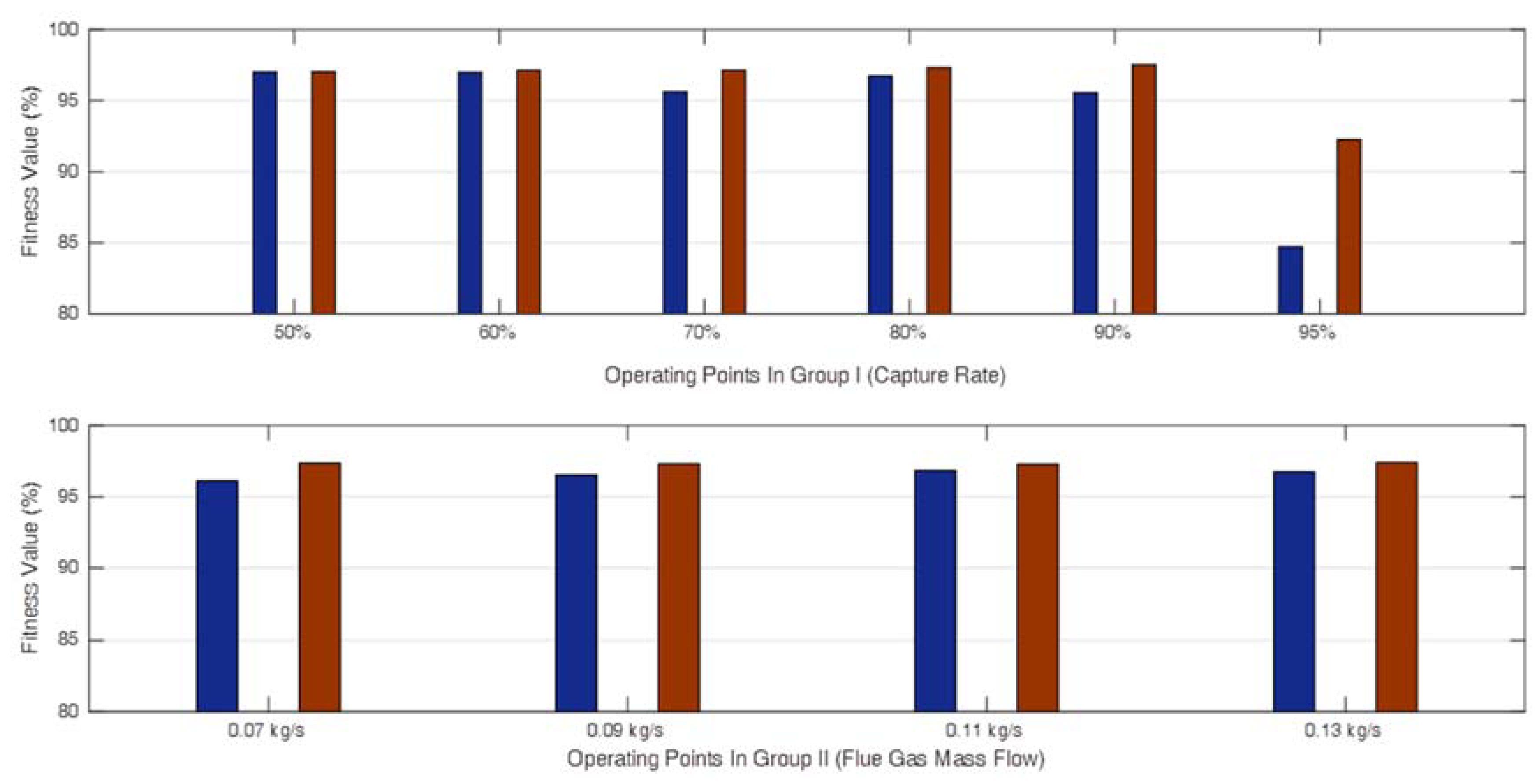
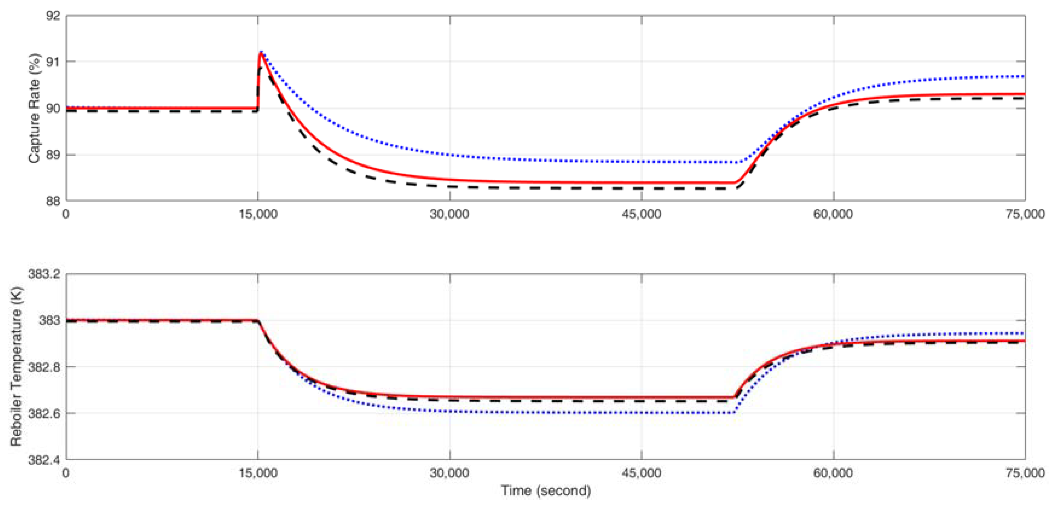
4.1. Validation of the Local Linear Models

In order to obtain the best identification results, random signals are implemented to the MEA-based CO₂ capture plant in the identification experiment of each local linear model. Considering the slow dynamics of the CO₂ capture process, the sampling time was chosen as 30 s. Taking the identification of 80% capture rate operating point model (in Group I) as an example, the input sequences for lean MEA flow rate and steam flow rate are plotted in Figure 8 and the identification results are presented in Figure 9. It can be seen that outputs of the local model are in good agreement with the plant. The fitness values of all the local models in Group I and Group II are plotted in Figure 10. The fitness value of the model is defined as:

$$FitnessValue=100\times (1-\frac{\sqrt{{{\displaystyle \sum }}_{k=1}^N(y_k-{\widehat{y_k}}^2)}}{\sqrt{{{\displaystyle \sum }}_{k=1}^N{\left(y_k-\overline{y}\right)}^2}}$$

(18)

where y_k and $\widehat{y_k}$ are the model outputs and plant measurements at time k, respectively, N is the number of validation data points, and $\overline{y}$ is the average of y_k.

As seen in Figure 10, the local linear models in Group I and Group II have very high fitness, which indicates that the local linear models can precisely predict the output of the CO₂ capture process around the selected operating point. Thus, the local linear models are qualified for the nonlinearity analysis and the establishment of the multi-linear model. Meanwhile, it can be seen that the model of the 95% capture rate in Group I has a slightly lower fitness value. This is because the process nonlinearity around 95% CO₂ capture rate is very strong and reduces the prediction accuracy of the single linear model.

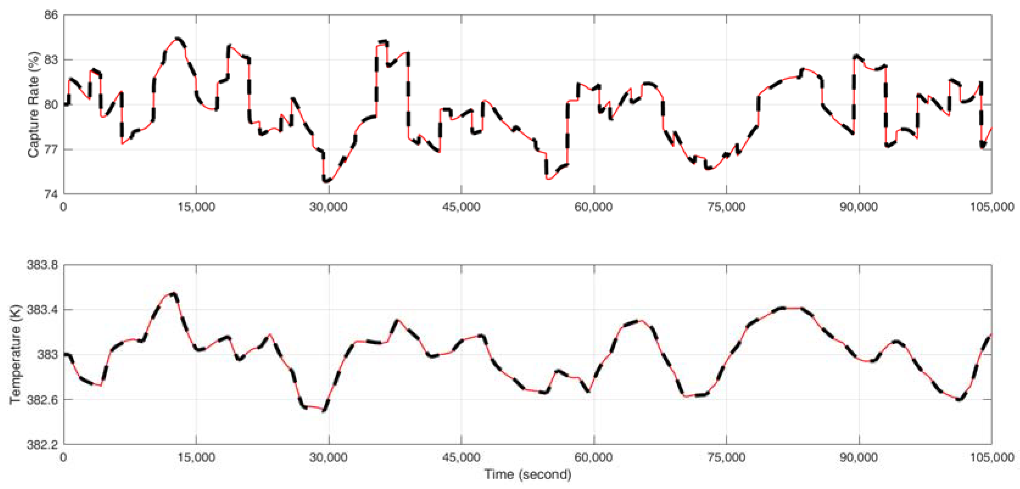
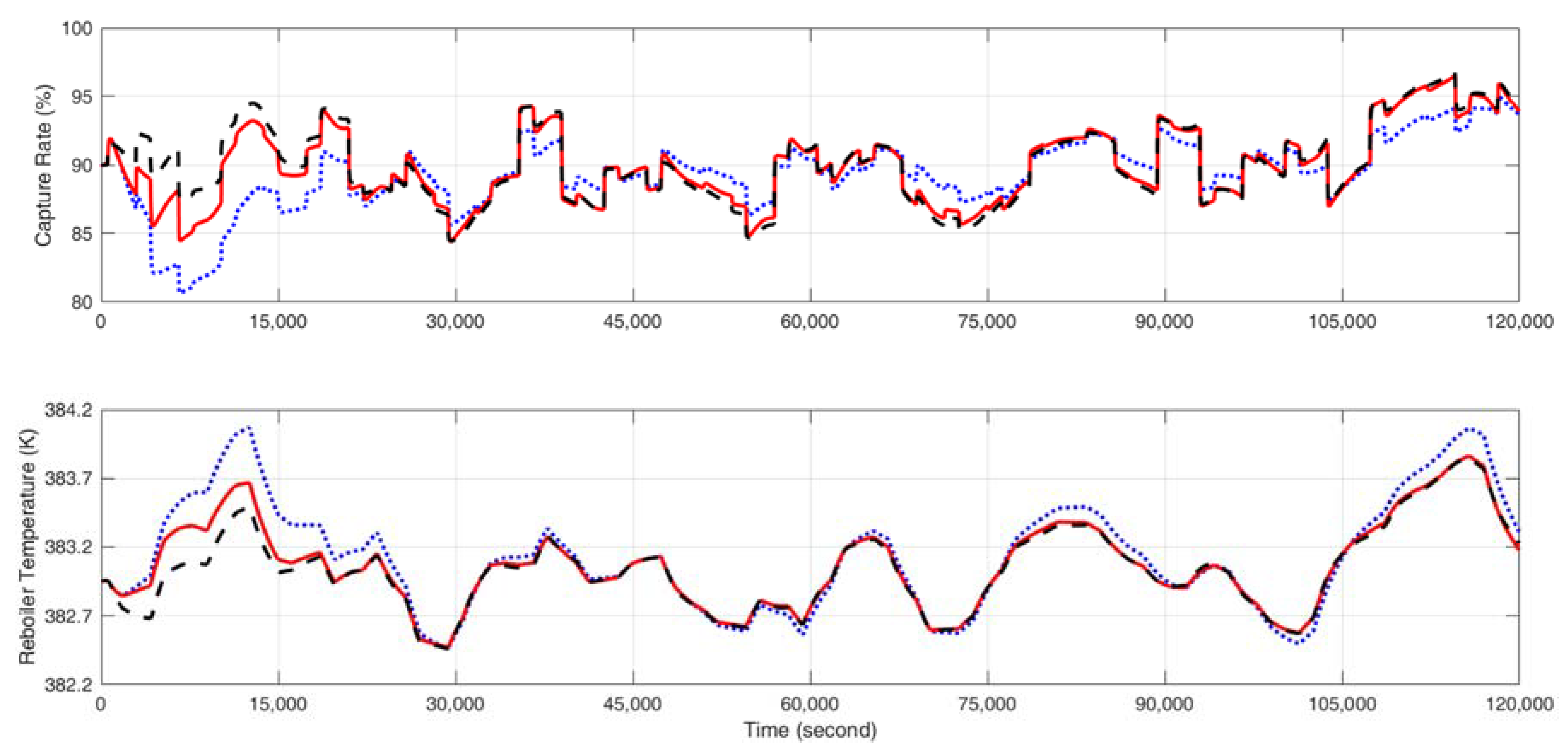
4.2. Validation of the Multi-Linear Model

In this section, the effectiveness of the proposed multi-linear model is tested via two simulation cases: response of step signal and response of random signal. In both cases, the flue gas mass flow rate is fixed at 0.13 kg/s. In the first case, the mass flow of lean solvent and extracted steam steps are applied at 15,000 s and 50,000 s, respectively. Since the process operates around 80% CO₂ capture rate, we chose the local linear model of 80% CO₂ capture rate for comparison. In the second case, we make the system operating in a wide operating range by imposing random input signals that fluctuate around the steady-state input of 70% CO₂ capture rate with a large amplitude. The local linear model with the 70% capture rate was selected for comparison. The input signals for Case I and Case II are shown in Figure 11 and Figure 12, respectively, and the corresponding validation outputs are presented in Figure 13 and Figure 14, respectively.

It can be observed in Figure 13 and Figure 14 that the proposed multi-linear has a very high prediction accuracy of the MEA-based post-combustion CO₂ capture process. Both the dynamic and steady-state behaviors of the process are precisely predicted with minor error. Therefore, the multi-linear model can achieve improved control performance when applied to model-based advanced control system design. Although the local linear model correctly captures the trends and time constant of the step response, it has large error in predicting the dynamics with random input signals, which will lead to the degradation of the control performance when the CO₂ capture plant operates flexibly under a wide operating range.

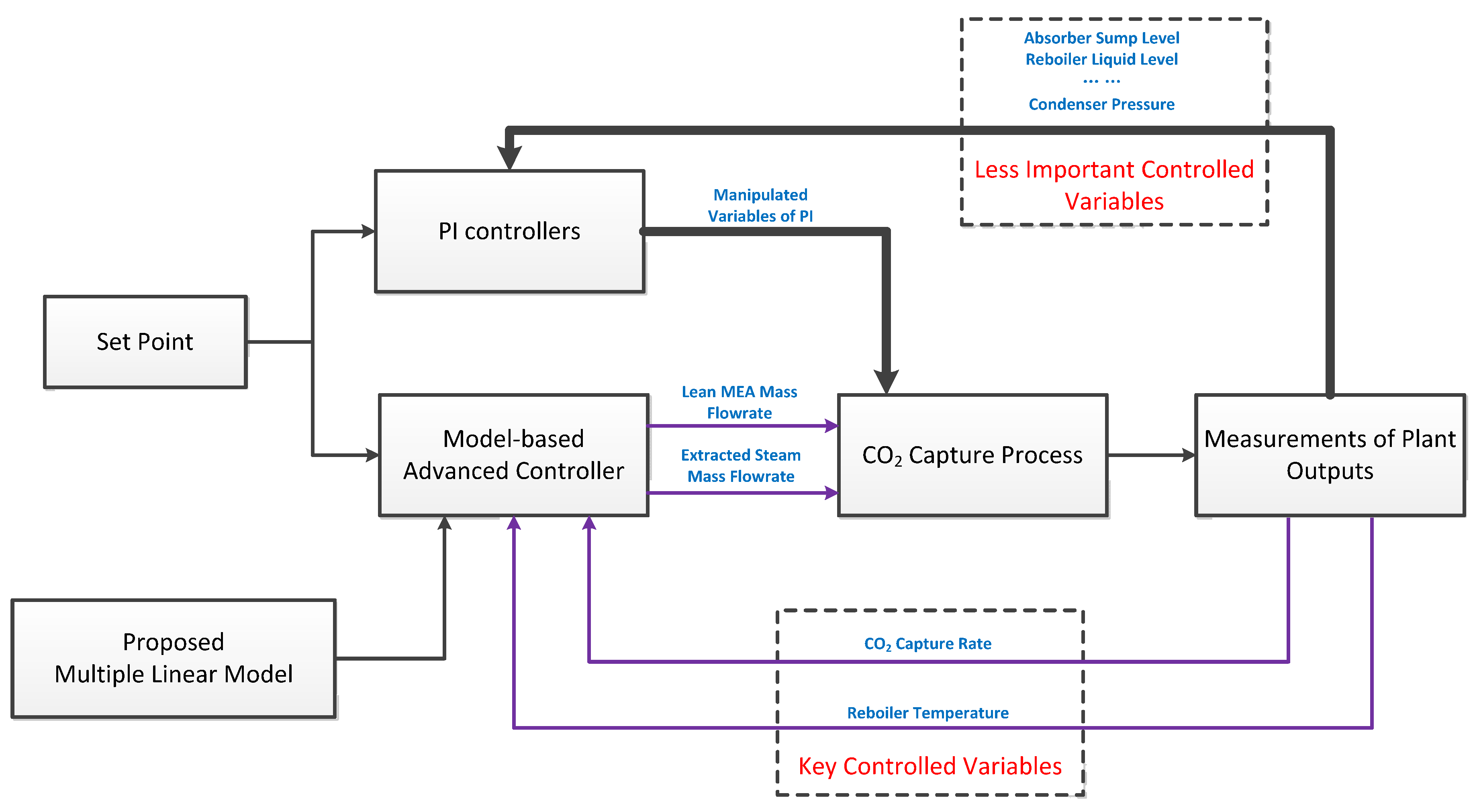
5. Introducing the Multi-Linear Model to Advanced Control System Design

Because the multi-linear model has high prediction accuracy and the desired state-space type of expression, it can be used in many practical advanced control techniques. In this section, the potential of the multi-linear model to be used in advanced control system designs for the MEA-based post-combustion CO₂ capture process is briefly discussed.

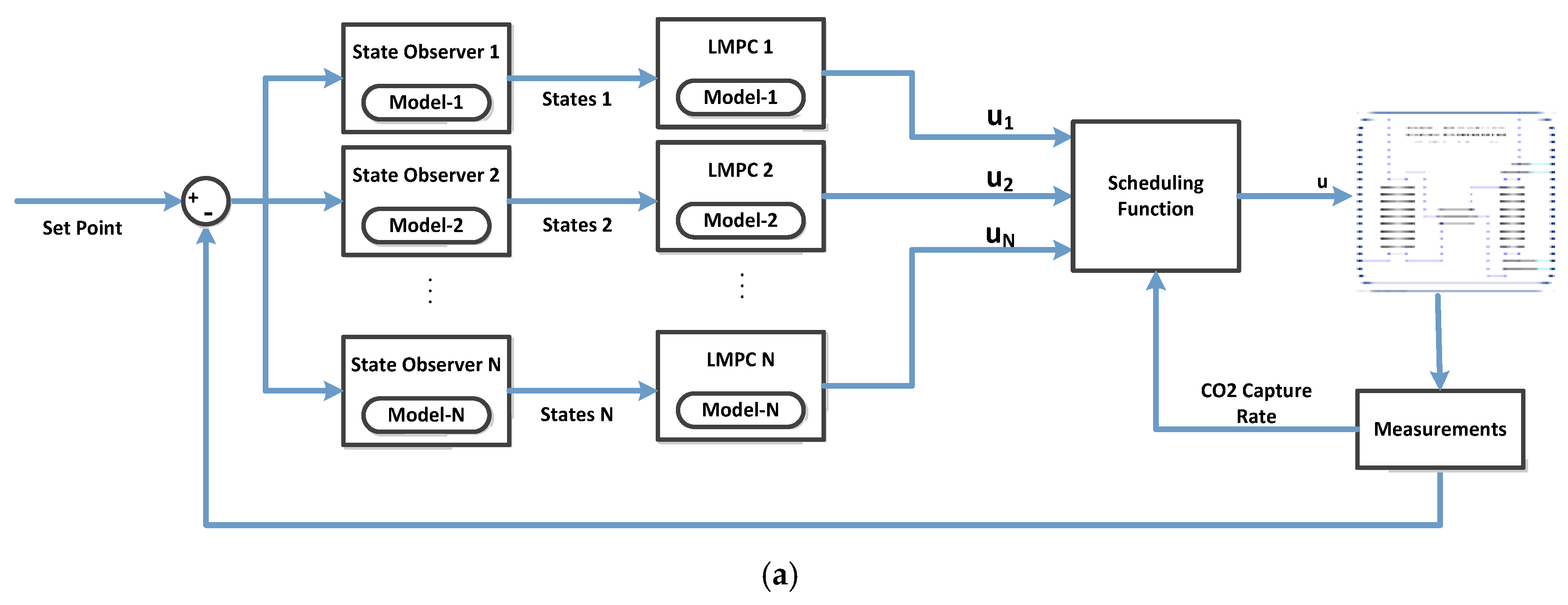
5.1. Multi-Model Predictive Control

The proposed multi-linear model predictive control (MMPC) can be seen as an upgraded version of linear model predictive control (LMPC). In MMPC, there are basically two methods to integrate the multi-linear model with the model predictive control (MPC) algorithm: the controller weighting method and the model weighting method. In the controller weighting method, the multi-linear model is utilized indirectly; multiple LMPCs are designed for each selected operating point and then the control move is calculated by weighting the outputs of the local LMPCs using the scheduling function of the multi-linear model [45]. The advantage of the controller weighting method is that the local controllers can be tuned easily based on the local linear models. In the model weighting method, the multi-linear model is directly used for prediction and only one controller is designed, which can reduce the online computational cost. However, the tuning of such a controller can be difficult, since the multi-linear model is actually time-varying. Hence, complex design algorithms which can guarantee the stability of the model weighting-based MMPC have been studied [49]. The control structures of the two methods are presented in Figure 15.

In practice, MMPC is more attractive than nonlinear model predictive control (NMPC), as it can be easily applied by modifying the LMPC algorithm. Moreover, the NMPC has the problem of local minimal solution and heavy online computational cost, which makes it a theoretical concept rather than a practical solution [50].

In comparison with LMPC, MMPC can significantly improve the flexibility of the CO₂ capture plant in a wide operating range, because it has a much better prediction model.

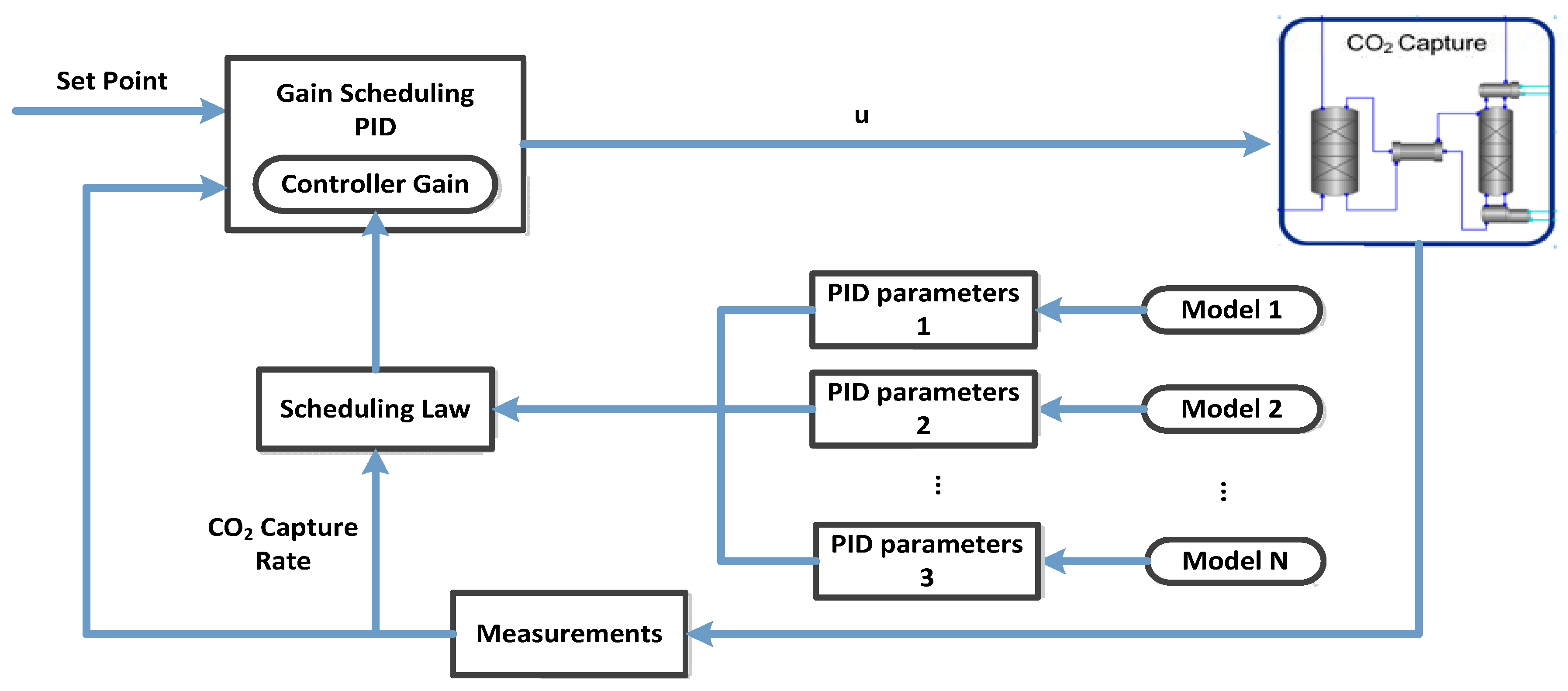
5.2. Gain Scheduling Proportional Integral Derivative Control

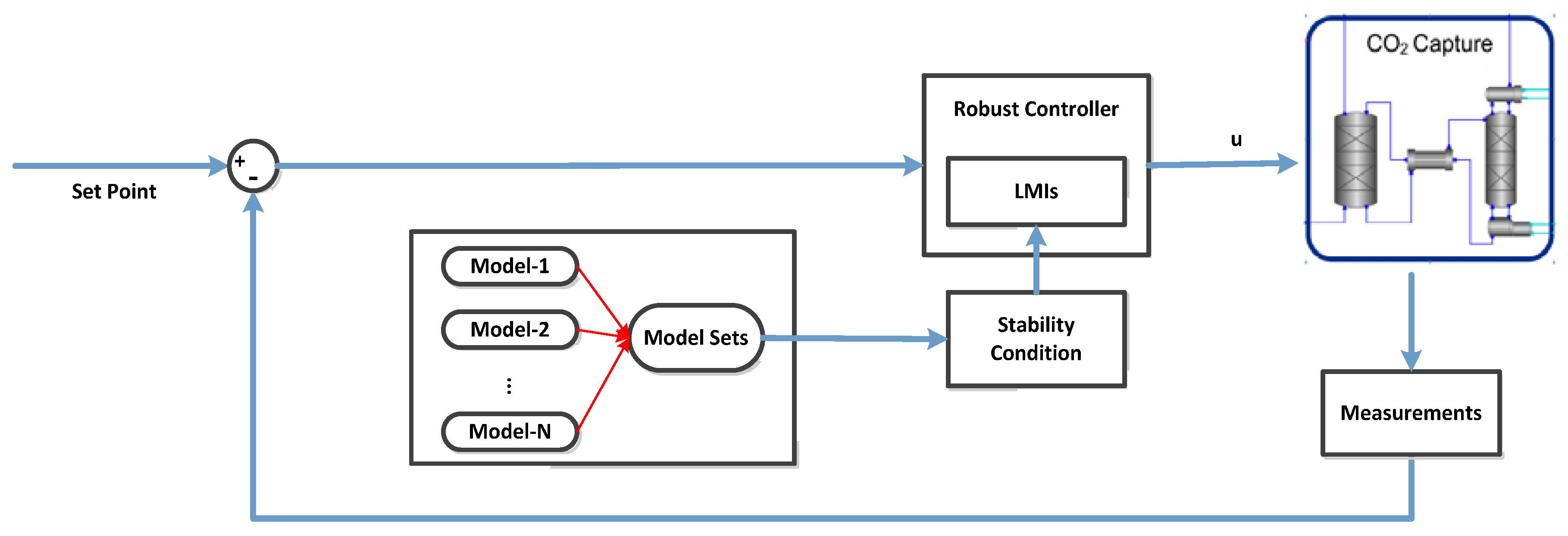
The multi-linear model is of high accuracy over the full operating range, thus the parameters of the proportional integral derivative (PID) controller can be tuned for each local linear model to reduce the influence of process nonlinearity. Furthermore, the parameters of the PID can be dynamically adjusted according to the change of the CO₂ capture rate, which results in the gain scheduling PID control. The gain scheduling law is generally designed using fuzzy logic [51], which can have a similar expression to the scheduling function of the multi-linear model. The gain scheduling PID can be conveniently applied to the real process without too much modification to the original PID control algorithm, and thus it can achieve a more robust control performance than nonlinear controllers. The control scheme of a gain scheduling PID is presented in Figure 16.

5.3. Robust Control

The multi-linear model provides a model set for designing the robust controller, which consists of all the possible combinations of the local linear models. In a robust control scheme, a Lyapunov function is formed to find the stability condition of the model sets, meanwhile ensuring a satisfactory transient performance of the system. With the Lyapunov function, a set of linear matrix inequalities (LMI) can be derived to design a stable controller for the model sets. Note that the LMI problems can be solved using many powerful numerical methods in a practical and efficient manner [52], making the robust control applicable for real engineering problems. The control structure of robust control is presented in Figure 17.

Remark 2.

The proposed multi-linear method can be applied to advanced control system design by modifying the linear control algorithms. Moreover, the multi-linear model can be easily constructed. Thus, the multi-model approach is very promising and practical to improve the existing linear control systems designed for the MEA-based CO₂ capture process. The control system for the CO₂ capture process based on multi-linear models will be studied in our future works.

6. Conclusions

To provide design foundations for advanced control systems to attain a wide range of flexible operation of the MEA-based post-combustion CO₂ capture process, this paper systematically studies the multi-model modeling approach for the CO₂ capture process. The local linear models are firstly identified at typical operating points via the subspace identification approach. Then the nonlinearity distribution of the process is investigated for two operating situations: the change of the CO₂ capture rate and the change of mass flow of the flue gas. Finally, the multi-linear model is developed based on the nonlinearity distribution. Simulation results demonstrate that the multi-linear model provides much more accurate predictions than the linear model. Moreover, the proposed multi-linear model has a suitable linear state-space type of expression, and thus can be employed directly for many applied advanced control techniques.

References

1. Bui, M.; Gunawan, I.; Verheyen, V.; Feron, P.; Meuleman, E.; Adeloju, S. Dynamic modelling and optimisation of flexible operation in post-combustion CO2 capture plants—A review. Comput. Chem. Eng. 2014, 61, 245–265. [Google Scholar] [CrossRef]
2. Lawal, A.; Wang, M.; Stephenson, P.; Koumpouras, G.; Yeung, H. Dynamic modelling and analysis of post-combustion CO2 chemical absorption process for coal-fired power plants. Fuel 2010, 89, 2791–2801. [Google Scholar] [CrossRef] [Green Version]
3. Lawal, A.; Wang, M.; Stephenson, P.; Obi, O. Demonstrating full-scale post-combustion CO2 capture for coal-fired power plants through dynamic modelling and simulation. Fuel 2012, 101, 115–128. [Google Scholar] [CrossRef] [Green Version]
4. Nittaya, T.; Douglas, P.L.; Croiset, E.; Ricardez-Sandoval, L.A. Dynamic modelling and control of MEA absorption processes for CO2 capture from power plants. Fuel 2014, 116, 672–691. [Google Scholar] [CrossRef]
5. Luu, M.T.; Manaf, N.A.; Abbas, A. Dynamic modelling and control strategies for flexible operation of amine-based post-combustion CO2 capture systems. Int. J. Greenh. Gas Control 2015, 39, 377–389. [Google Scholar] [CrossRef]
6. He, Z.; Sahraei, M.H.; Ricardez-Sandoval, L.A. Flexible operation and simultaneous scheduling and control of a CO2 capture plant using model predictive control. Int. J. Greenh. Gas Control 2016, 48, 300–311. [Google Scholar] [CrossRef]
7. Wellner, K.; Marx-Schubach, T.; Schmitz, G. Dynamic behavior of coal-fired power plants with postcombustion CO2 capture. Ind. Eng. Chem. Res. 2016, 55, 12038–12045. [Google Scholar] [CrossRef]
8. Walters, M.S.; Edgar, T.F.; Rochelle, G.T. Dynamic modeling and control of an intercooled absorber for post-combustion CO2 capture. Chem. Eng. Process. Process Intensif. 2016, 107, 1–10. [Google Scholar] [CrossRef]
9. Posch, S.; Haider, M. Dynamic modeling of CO2 absorption from coal-fired power plants into an aqueous monoethanolamine solution. Chem. Eng. Res. Des. 2013, 91, 977–987. [Google Scholar] [CrossRef]
10. Ziaii, S.; Rochelle, G.T.; Edgar, T.F. Dynamic modeling to minimize energy use for CO2 capture in power plants by aqueous monoethanolamine. Ind. Eng. Chem. Res. 2009, 48, 6105–6111. [Google Scholar] [CrossRef]
11. Mac Dowell, N.; Samsatli, N.J.; Shah, N. Dynamic modelling and analysis of an amine-based post-combustion CO2 capture absorption column. Int. J. Greenh. Gas Control 2013, 12, 247–258. [Google Scholar] [CrossRef]
12. Léonard, G.; Mogador, B.C.; Belletante, S.; Heyen, G. Dynamic modelling and control of a pilot plant for post-combustion CO2 capture. In Computer Aided Chemical Engineering; Elsevier: Amsterdam, The Netherlands, 2013; Volume 32, pp. 451–456. [Google Scholar]
13. Lawal, A.; Wang, M.; Stephenson, P.; Yeung, H. Dynamic modelling of CO2 absorption for post combustion capture in coal-fired power plants. Fuel 2009, 88, 2455–2462. [Google Scholar] [CrossRef] [Green Version]
14. Manaf, N.A.; Cousins, A.; Feron, P.; Abbas, A. Dynamic modelling, identification and preliminary control analysis of an amine-based post-combustion CO2 capture pilot plant. J. Clean. Prod. 2016, 113, 635–653. [Google Scholar] [CrossRef]
15. Van De Haar, A.; Trapp, C.; Wellner, K.; De Kler, R.; Schmitz, G.; Colonna, P. Dynamics of postcombustion CO2 capture plants: Modeling, validation, and case study. Ind. Eng. Chem. Res. 2017, 56, 1810–1822. [Google Scholar] [CrossRef] [PubMed]
16. Lin, Y.-J.; Wong, D.S.-H.; Jang, S.-S.; Ou, J.-J. Control strategies for flexible operation of power plant with CO2 capture plant. AIChE J. 2012, 58, 2697–2704. [Google Scholar] [CrossRef]
17. Sahraei, M.H.; Ricardez-Sandoval, L.A. Controllability and optimal scheduling of a CO2 capture plant using model predictive control. Int. J. Greenh. Gas Control 2014, 30, 58–71. [Google Scholar] [CrossRef]
18. Agbonghae, E.O.; Hughes, K.J.; Ingham, D.B.; Ma, L.; Pourkashanian, M. Optimal process design of commercial-scale amine-based CO2 capture plants. Ind. Eng. Chem. Res. 2014, 53, 14815–14829. [Google Scholar] [CrossRef]
19. Arce, A.; Mac Dowell, N.; Shah, N.; Vega, L.F. Flexible operation of solvent regeneration systems for CO2 capture processes using advanced control techniques: Towards operational cost minimisation. Int. J. Greenh. Gas Control 2012, 11, 236–250. [Google Scholar] [CrossRef]
20. Garđarsdóttir, S.O.; Montañés, R.M.; Normann, F.; Nord, L.O.; Johnsson, F. Effects of CO2-absorption control strategies on the dynamic performance of a supercritical pulverized-coal-fired power plant. Ind. Eng. Chem. Res. 2017, 56, 4415–4430. [Google Scholar] [CrossRef]
21. Afkhamipour, M.; Mofarahi, M. Sensitivity analysis of the rate-based CO2 absorber model using amine solutions (MEA, MDEA and AMP) in packed columns. Int. J. Greenh. Gas Control 2014, 25, 9–22. [Google Scholar] [CrossRef]
22. Zhang, Y.; Chen, H.; Chen, C.-C.; Plaza, J.M.; Dugas, R.; Rochelle, G.T. Rate-based process modeling study of CO2 capture with aqueous monoethanolamine solution. Ind. Eng. Chem. Res. 2009, 48, 9233–9246. [Google Scholar] [CrossRef]
23. Gabrielsen, J.; Svendsen, H.F.; Michelsen, M.L.; Stenby, E.H.; Kontogeorgis, G.M. Experimental validation of a rate-based model for CO2 capture using an AMP solution. Chem. Eng. Sci. 2007, 62, 2397–2413. [Google Scholar] [CrossRef]
24. Mores, P.; Scenna, N.; Mussati, S. A rate based model of a packed column for CO2 absorption using aqueous monoethanolamine solution. Int. J. Greenh. Gas Control 2012, 6, 21–36. [Google Scholar] [CrossRef]
25. Niu, Z.; Guo, Y.; Zeng, Q.; Lin, W. Experimental studies and rate-based process simulations of CO2 absorption with aqueous ammonia solutions. Ind. Eng. Chem. Res. 2012, 51, 5309–5319. [Google Scholar] [CrossRef]
26. Plaza, J.M.; Van Wagener, D.; Rochelle, G.T. Modeling CO2 capture with aqueous monoethanolamine. Int. J. Greenh. Gas Control 2010, 4, 161–166. [Google Scholar] [CrossRef]
27. Borhani, T.N.G.; Akbari, V.; Afkhamipour, M.; Hamid, M.K.A.; Manan, Z.A. Comparison of equilibrium and non-equilibrium models of a tray column for post-combustion CO2 capture using DEA-promoted potassium carbonate solution. Chem. Eng. Sci. 2015, 122, 291–298. [Google Scholar] [CrossRef]
28. Yokoyama, T. Analysis of reboiler heat duty in MEA process for CO2 capture using equilibrium-staged model. Sep. Purif. Technol. 2012, 94, 97–103. [Google Scholar] [CrossRef]
29. Qin, S.J.; Badgwell, T.A. An overview of nonlinear model predictive control applications. In Nonlinear Model Predictive Control; Springer: New York, NY, USA, 2000; pp. 369–392. [Google Scholar]
30. Zhang, Q.; Turton, R.; Bhattacharyya, D. Development of model and model-predictive control of an MEA-based postcombustion CO2 capture process. Ind. Eng. Chem. Res. 2016, 55, 1292–1308. [Google Scholar] [CrossRef]
31. Sipöcz, N.; Tobiesen, F.A.; Assadi, M. The use of artificial neural network models for CO2 capture plants. Appl. Energy 2011, 88, 2368–2376. [Google Scholar] [CrossRef]
32. Li, F.; Zhang, J.; Oko, E.; Wang, M. Modelling of a post-combustion CO2 capture process using neural networks. Fuel 2015, 151, 156–163. [Google Scholar] [CrossRef]
33. Bai, Z.; Li, F.; Zhang, J.; Oko, E.; Wang, M.; Xiong, Z.; Huang, D. Modelling of a post-combustion CO2 capture process using bootstrap aggregated extreme learning machines. In Computer Aided Chemical Engineering; Elsevier: Amsterdam, The Netherlands, 2016; Volume 38, pp. 2007–2012. [Google Scholar]
34. Du, J.; Johansen, T.A. Integrated multilinear model predictive control of nonlinear systems based on gap metric. Ind. Eng. Chem. Res. 2015, 54, 6002–6011. [Google Scholar] [CrossRef]
35. Du, J.; Song, C.; Yao, Y.; Li, P. Multilinear model decomposition of MIMO nonlinear systems and its implication for multilinear model-based control. J. Process Control 2013, 23, 271–281. [Google Scholar] [CrossRef]
36. Mechleri, E.; Lawal, A.; Ramos, A.; Davison, J.; Mac Dowell, N. Process control strategies for flexible operation of post-combustion CO2 capture plants. Int. J. Greenh. Gas Control 2017, 57, 14–25. [Google Scholar] [CrossRef]
37. Putta, K.R.; Knuutila, H.; Svendsen, H.F. Activity based kinetics and mass transfer of CO2 absorption into MEA using penetration theory. Energy Procedia 2014, 63, 1196–1205. [Google Scholar] [CrossRef]
38. Chapman, W.G.; Gubbins, K.E.; Jackson, G.; Radosz, M. SAFT: Equation-of-state solution model for associating fluids. Fluid Phase Equilib. 1989, 52, 31–38. [Google Scholar] [CrossRef]
39. Lin, Y.-J.; Pan, T.-H.; Wong, D.S.-H.; Jang, S.-S.; Chi, Y.-W.; Yeh, C.-H. Plantwide control of CO2 capture by absorption and stripping using monoethanolamine solution. Ind. Eng. Chem. Res. 2010, 50, 1338–1345. [Google Scholar] [CrossRef]
40. Ziegler, J.G. Optimum settings for automatic controllers. Asme Trans 1993, 64, 759–768. [Google Scholar] [CrossRef]
41. Katayama, T. Subspace Methods for System Identification; Springer Science & Business Media: Berlin/Heidelberg, Germany, 2006. [Google Scholar]
42. Wu, X.; Shen, J.; Li, Y.; Lee, K.Y. Data-driven modeling and predictive control for boiler-turbine unit using fuzzy clustering and subspace methods. ISA Trans. 2014, 53, 699–708. [Google Scholar] [CrossRef] [PubMed]
43. Zames, G. Unstable systems and feedback: The gap metric. In Proceedings of the Allerton Conference, Monticello, IL, USA, 8–10 October 1980; pp. 380–385. [Google Scholar]
44. Qui, L.; Davison, E.J. Feedback stability under simultaneous gap metric uncertainties in plant and controller. Syst. Control Lett. 1992, 18, 9–22. [Google Scholar] [CrossRef]
45. Du, J.; Johansen, T.A. A gap metric based weighting method for multimodel predictive control of MIMO nonlinear systems. J. Process Control 2014, 24, 1346–1357. [Google Scholar] [CrossRef]
46. Galan, O.; Romagnoli, J.A.; Arkun, Y.; Palazoglu, A. On the use of gap metric for model selection in multilinear model-based control. In Proceedings of the 2000 American Control Conference, Chicago, IL, USA, 28–30 June 2000; Volume 6, pp. 3742–3746. [Google Scholar]
47. Tao, X.; Li, D.; Wang, Y.; Li, N.; Li, S. Gap-metric-based multiple-model Predictive control with a polyhedral stability region. Ind. Eng. Chem. Res. 2015, 54, 11319–11329. [Google Scholar] [CrossRef]
48. Schach, M.; Schneider, R.; Schramm, H.; Repke, J. Control structure design for CO2-absorption processes with large operating ranges. Energy Technol. 2013, 1, 233–244. [Google Scholar] [CrossRef]
49. Wu, X.; Shen, J.; Li, Y.; Lee, K.Y. Fuzzy modeling and stable model predictive tracking control of large-scale power plants. J. Process Control 2014, 24, 1609–1626. [Google Scholar] [CrossRef]
50. Camacho, E.F.; Bordons, C. Nonlinear model predictive control. In Model Predictive Control; Springer: New York, NY, USA, 2007; pp. 249–288. [Google Scholar]
51. Blanchett, T.P.; Kember, G.C.; Dubay, R. PID gain scheduling using fuzzy logic. ISA Trans. 2000, 39, 317–325. [Google Scholar] [CrossRef]
52. El Ghaoui, L.; Niculescu, S. Advances in Linear Matrix Inequality Methods in Control; SIAM: Philadelphia, PA, USA, 2000. [Google Scholar]
Figure 1. Monoethanolamine (MEA)-based post-combustion CO2 capture plant topology.
Applsci 08 01053 g001
Figure 2. Liquid and vapor bulks, films, and interface (Vb: vapour bulk; V: vapour; VI: vapour interface; Vf: vapour film; Lb: liquid bulk; L: liquid; LI: liquid interface; Lf: liquid film).
Applsci 08 01053 g002
Figure 3. Overall control structure of the CO2 capture process. PI: proportional integral.
Applsci 08 01053 g003
Figure 4. Gap metric of the neighboring operating points with different CO2 capture rates.
Applsci 08 01053 g004
Figure 5. Gap metric of the neighboring operating points with different flue gas flow rates.
Applsci 08 01053 g005
Figure 6. Trapezoidal scheduling functions (the blue line represents the scheduling function of the 50% capture rate model, the red line represents the scheduling function of the 80% capture rate model, the purple line represents the scheduling function of the 95% capture rate model).
Applsci 08 01053 g006
Figure 7. Formulation of the multi-linear model.
Applsci 08 01053 g007
Figure 8. Identification signals for the operating point of 80% capture rate (in Group I).
Applsci 08 01053 g008
Figure 9. Validation results for the operating point of 80% capture rate (solid lines: model output; dashed lines: measurements from the process).
Applsci 08 01053 g009
Figure 10. Fitness value of the local models (blue lines: fitness of CO2 capture rate; red lines: fitness of reboiler temperature).
Applsci 08 01053 g010
Figure 11. Input signals for Case I.
Applsci 08 01053 g011
Figure 12. Input signals for Case II.
Applsci 08 01053 g012
Figure 13. Model validation results for Case I (solid line in red: the multi-linear model; dotted line in blue: the local linear model; dashed line in black: process measurement).
Applsci 08 01053 g013
Figure 14. Model validation results for Case II (solid line in red: the multi-linear model; dotted line in blue: the local linear model; dashed line in black: process measurement.).
Applsci 08 01053 g014
Figure 15. Control structure of multi-model predictive control (MMPC); linear model predictive control (LMPC). (a) Controller weighting method; (b) Model weighting method.
Applsci 08 01053 g015aApplsci 08 01053 g015b
Figure 16. Control structure of gain scheduling control. PID: proportional integral derivative.
Applsci 08 01053 g016
Figure 17. Control structure of robust control. LMIs: linear matrix inequalities.
Applsci 08 01053 g017