Article

A UAV-Based Visual Inspection Method for Rail Surface Defects

1
State Key Laboratory of Rail Traffic Control and Safety, Beijing Jiaotong University, Beijing 100044, China
2
School of Traffic and Transportation, Beijing Jiaotong University, Beijing 100044, China
3
Beijing Research Center of Urban Traffic Information Sensing and Service Technologies, Beijing 100044, China
*
Authors to whom correspondence should be addressed.
Appl. Sci. 2018, 8(7), 1028; https://doi.org/10.3390/app8071028
Submission received: 29 May 2018 / Revised: 15 June 2018 / Accepted: 21 June 2018 / Published: 24 June 2018
(This article belongs to the Special Issue Intelligent Imaging and Analysis)

Abstract

:
Rail surface defects seriously affect the safety of railway systems. At present, human inspection and rail vehicle inspection are the main approaches for the detection of rail surface defects. However, there are many shortcomings to these approaches, such as low efficiency, high cost, and so on. This paper presents a novel visual inspection approach based on unmanned aerial vehicle (UAV) images, and focuses on two key issues of UAV-based rail images: image enhancement and defects segmentation. With regards to the first aspect, a novel image enhancement algorithm named Local Weber-like Contrast (LWLC) is proposed to enhance rail images. The rail surface defects and backgrounds can be highlighted and homogenized under various sunlight intensity by LWLC, due to its illuminance independent, local nonlinear and other advantages. With regards to the second, a new threshold segmentation method named gray stretch maximum entropy (GSME) is presented in this paper. The proposed GSME method emphasizes gray stretch and de-noising on UAV-based rail images, and selects an optimal segmentation threshold for defects detection. Two visual comparison experiments were carried out to demonstrate the efficiency of the proposed methods. Finally, a quantitative comparison experiment shows the LWLC-GSME model achieves a recall of 93.75% for T-I defects and of 94.26% for T-II defects. Therefore, LWLC for image enhancement, in conjunction with GSME for defects segmentation, is efficient and feasible for the detection of rail surface defects based on UAV Images.

1. Introduction

Rail transportation plays a significant role in the development of economic and industrial growth, and the failures of railway facilities (such as defects on the rail surface) are directly related to catastrophic accidents [1]. With the development of high-speed and high-load rail transit, the probability of rail surface defects is increasing rapidly. In general, rail surface defects which include corrugations and discrete defects due to wheel-rail contact conditions are the most common forms of defects [2]. Corrugations arise from periodic slip of the wheel on the rail as trains run on tracks [3]. The discrete defects are generated on the rail surface in an apparently random manner, i.e., without periodic characteristics, as shown in Figure 1. Those defects might cause serious accidents, or may even result in a catastrophic derailment of vehicles. Thus, this paper mainly discusses the detection of surface discrete defects.
Currently, there are regular inspections of tracks in order to maintain safe and efficient operation [4]. Historically, inspection tasks are performed by trained personnel, by walking along the tracks. However, the manual inspection is inappropriate due to its low-efficiency, lack of objectivity, and high false alarm rate. Furthermore, the results are seriously dependent on the capability of the observer to detect possible anomalies and recognize critical conditions [5]. Therefore, automatic and nondestructive inspection methods should be urgently developed.
At present, nondestructive inspection methods have been widely developed in a variety of industry inspection applications, due to their high efficiency and high precision [6]. Several methods have been applied to rail defects inspection, such as acoustic emission inspection [7], electromagnetic inspection [8], ultrasonic surface waves inspection [9], and visual inspection(VI) [10,11,12]. Particularly, with the development of computer vision techniques, VI (visual inspection) has been widely applied. VI is the most notable method for the surface defect detection because of its high speed and low cost [13]. Some researchers have studied rail surface defects by VI [14,15,16]. The VI method is an attractive approach for discrete defect detection.
According to the traditional VI approach for surface defects inspection, a high definition (HD) camera is used to capture rail images; it is embedded in a detection system installed under an inspection train. Currently, most related researches are based on this approach. However, it has inevitable drawbacks, such as limited detection range, high cost, and so on. Inspection trains have to run over significant distances to capture rail images for a wide range of detection. The detectable parts and viewing angles are limited, especially for mountainous areas or across rivers.
Unmanned Aerial Vehicles (UAVs) have become a research hotspot in many fields. The UAV-based inspection scheme is efficient and cost-effective, and has become attractive for change inspection in small-scale regions [17]. With the rapid development of UAVs, UAV-based aerial photography has been widely employed for engineering surveying and mapping [18], crop measurements [19], wind turbine blade surface inspection [20], power facilities inspection [21], historical buildings inspection [22], forest fire detection [23], bridge crack detection [24], fault detection in photovoltaic cells [25], and other detection applications such as target tracking [26], tracking and classification of multiple moving objects [27] and object recognition [28], etc. In general, UAV-based aerial photography has been extensively applied in various industries due to its advantages: low cost, ease of control, and flexibility.
As mentioned, an inspection method of rail surface defects based on UAV combined with VI is proposed in this paper. A typical approach to detect surface defects is to automatically extract defects after image enhancement [15]. The most two popular methods for image enhancement are by the histogram equalization (HE) and homomorphic filtering algorithms. However, since the HE is a linear algorithm and only averages the gray level distribution rather than enlarging the gray scale, there are several shortcomings, such as loss of image detail information and noise amplification [29]. Homomorphic filtering algorithm based on the illumination reflectance model is a frequency-domain processing to compress image light regions and enhance contrast. This method makes use of the frequency information of images. However, it often blurs image details, leading to a lack of deliberation of the spatial local characteristics of images [29]. In addition, gray values in the global scope change dramatically because of the uneven illumination and reflectance properties of rail surfaces [14]. Therefore, the two global enhancement methods are not suitable for rail images.
For defect detection, research on models that automatically locate defects after image enhancement has several achievements. For instance, a visual inspection system (VIS) is proposed for discrete defect detection [14]. In the VIS, images are captured by a high-speed digital camera fixed on a train. Subsequently, track extraction based on projection profile (TEBP) algorithm is used to extract the areas of rail track in images, and then the local normalized (LN) method and the defect localization based on projection profile (DLBP) method are applied to detect rail surface defects. The MLC-PEME model is proposed for defect detection [30]. Firstly, the histogram-based track extraction (HBTE) algorithm is used to extract areas of rail track in images which were captured by a camera fixed on an inspection train, then the MLC (Michelson-like contrast) combined with proportion emphasized maximum entropy (PEME) method is applied to detect defects. These methods performed well; however, they are seriously influenced by noise and background points, and consequently, have massive false detection rates [15]. An inverse PM diffusion model is proposed to enhance images [16]. Therefore, an adaptive threshold binarization is able to readily locate surface defects. However, it is seriously influenced by noise points, and yields in high false detection rates [15].
Most inspection models are based on the VI system fixed on inspection trains, and research on the UAV-based inspection of rail surface defects is rarely discussed. In this study, we faced the following serious challenges:
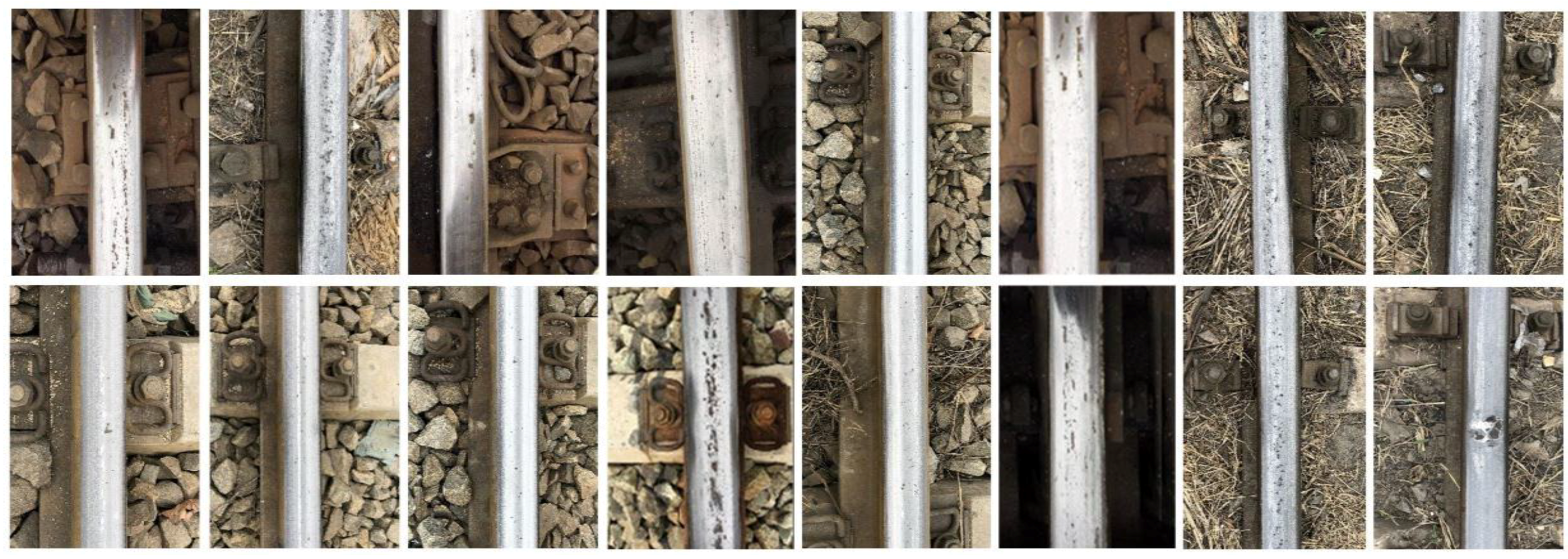
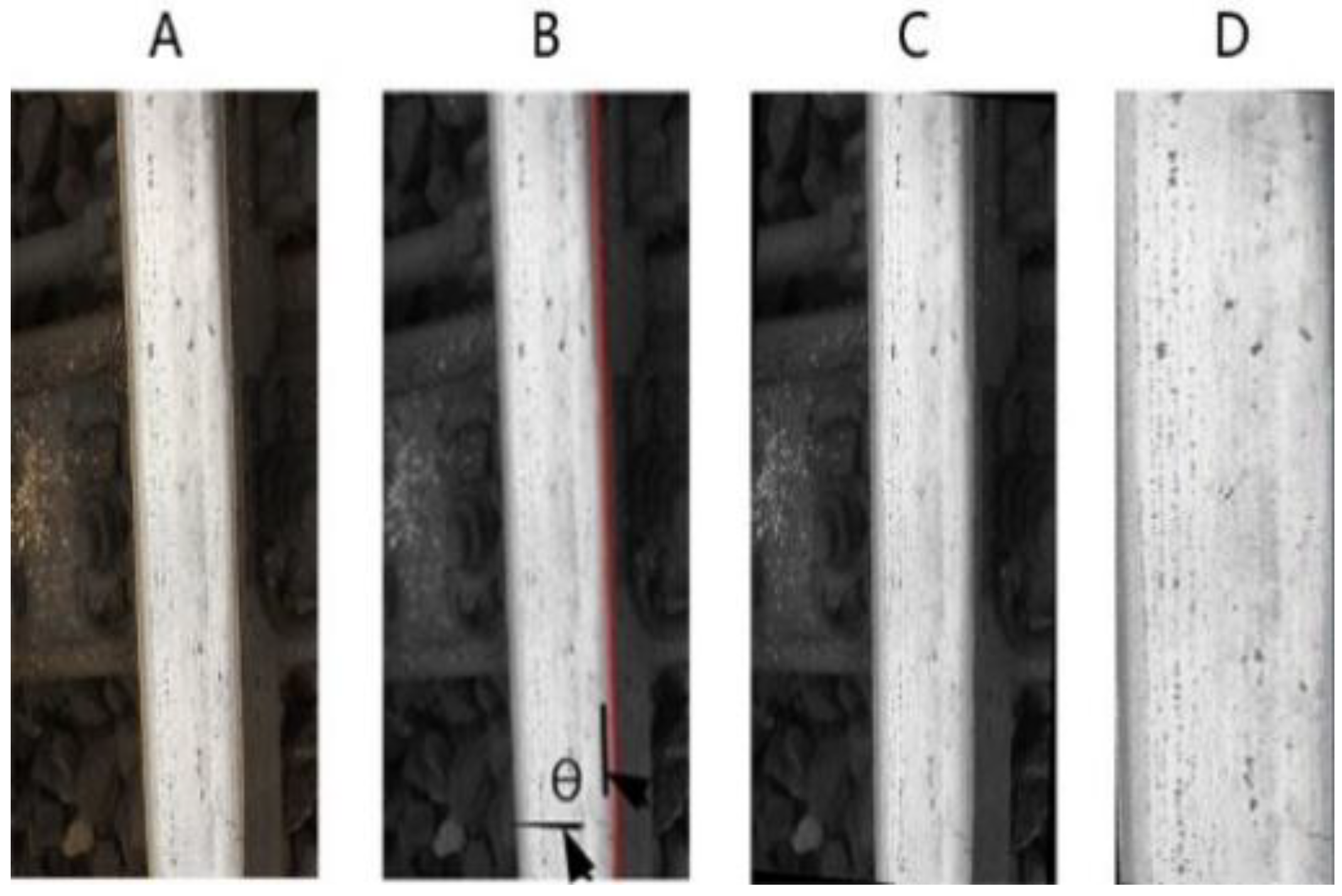
  • Rail position variances in UAV images. Unlike inspection trains, the camera angle of HD camera installed on UAV is sensitive to environment aspects (such as wind and turbulence) and operators. Although the UAV can balance itself by using GPS flight mode, rail positions in images captured by UAV aerial photography are extremely variable. Therefore, the variances of rail positions bring difficulties to rail extraction.
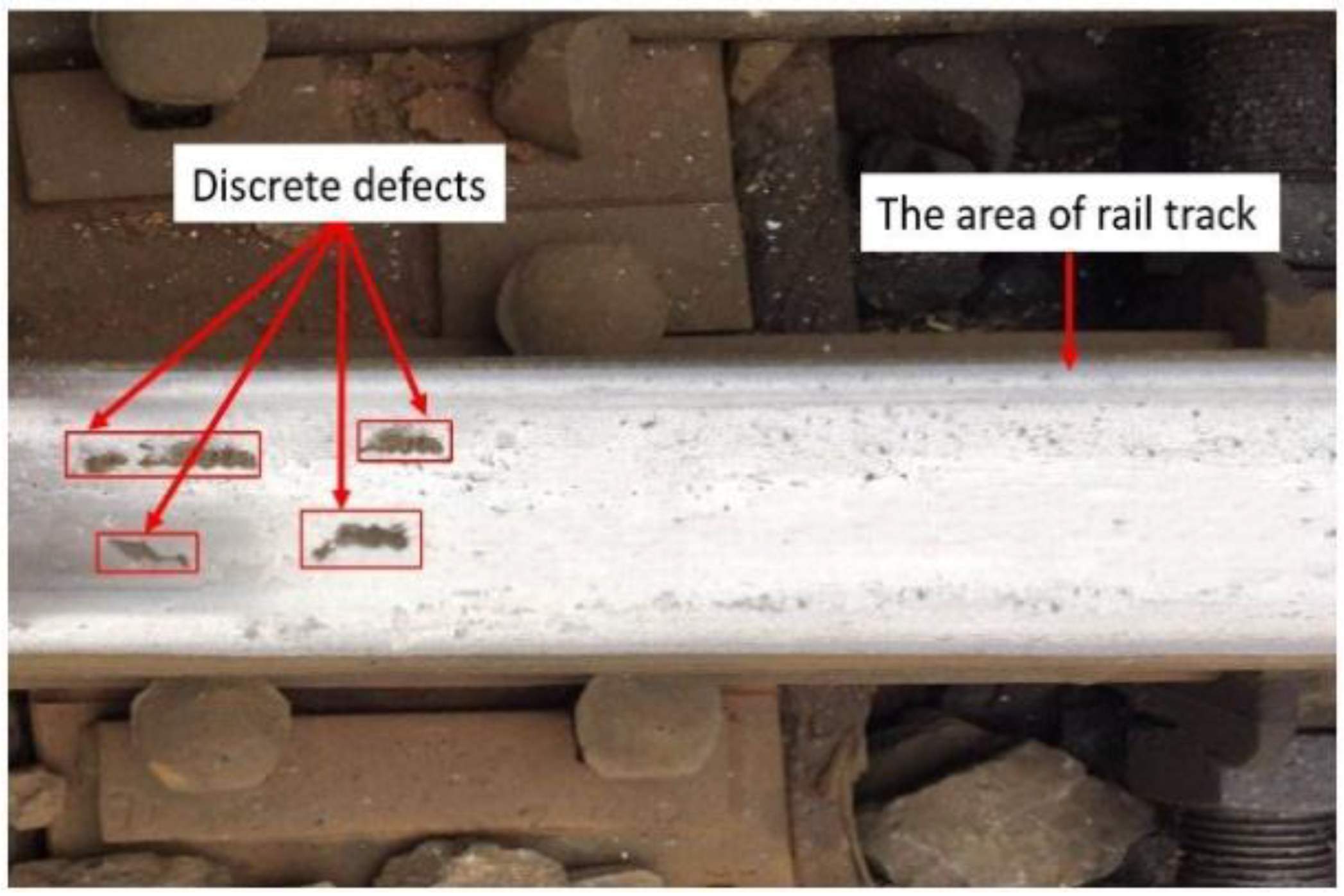
  • Non-uniform illumination and noise corruption. Due to partial occlusion of infrastructures around the rail (such as catenary etc.), reflectance properties of rail surface and shake of the UAV and other environmental factors, the brightness and contrast of images are uneven and low. According to [17,31], UAV digital images are likely to be corrupted by noises during the acquisition or transmission. In general, the gray levels of surface defects are lower than that of background (non-defect area) [14], but the order of these values is often broken because of non-uniform illumination and noise corruption, as shown in the Figure 1.
  • Few characteristics for defects segmentation. A corrugation initiates and develops easily because of the periodic occurrence of contact vibration [32]. However, it is difficult to inspect discrete defects by the VI method due to the lack of periodicity. Surface defects have low grey-level, that distinguishes them from the dynamic background. Therefore, the grey-level is considered to be the most available feature [14]. Therefore, the existing object recognition methods based on sophisticated texture and shape features are unfeasible, due to the limitation of visual features [15].
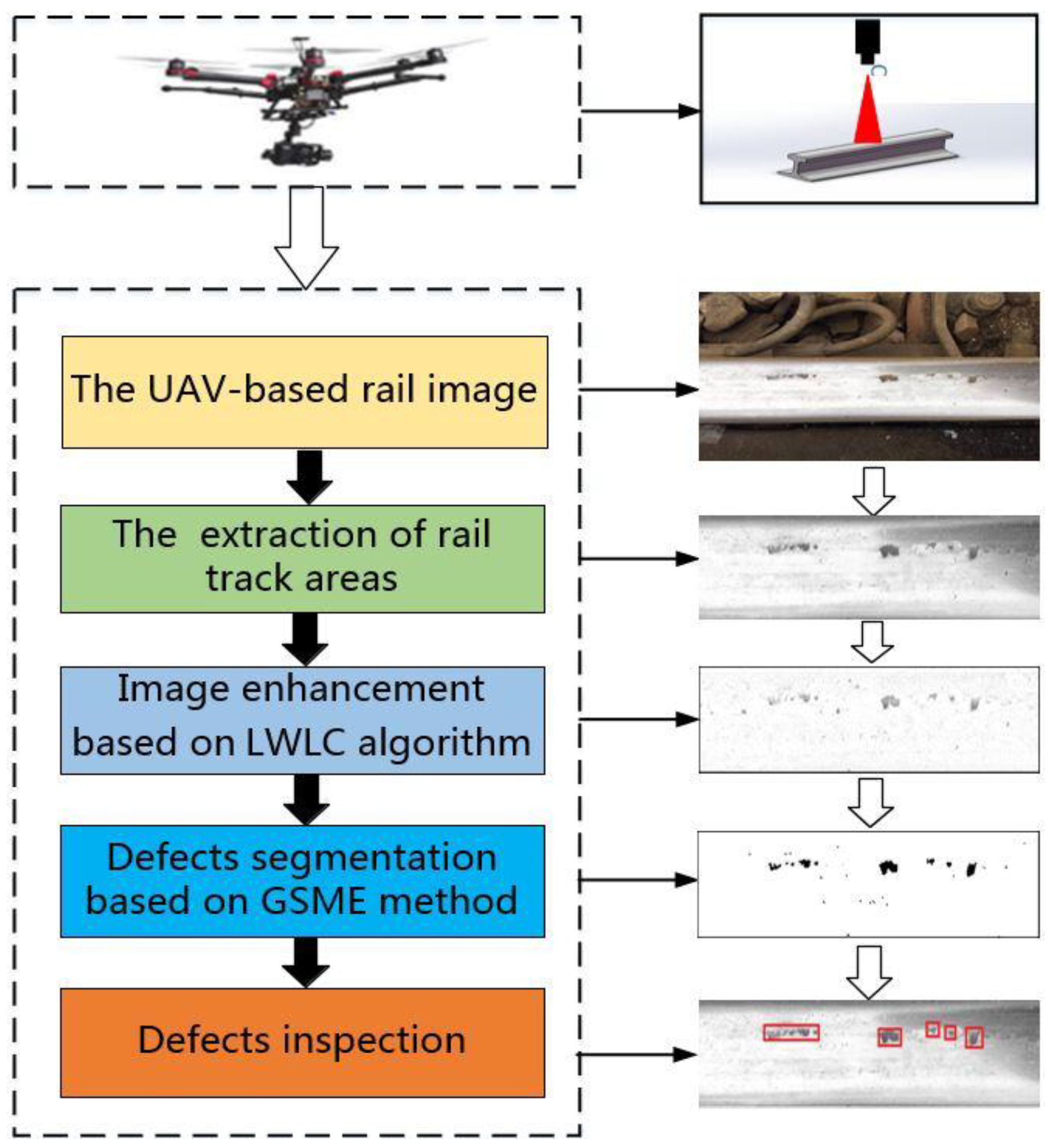
Also, due to the above challenges, these inspection models based on inspection trains are unable to be used in the case of UAV rail images. To overcome these challenges, this paper presents a novel image enhancement algorithm based on Weber’s law and a new threshold segmentation method based on the gray stretch in wavelet domain.
Weber’s law was first proposed by German physiologist Weber, and later formulated quantitatively as a mathematical expression referred to as Weber contrast by psychologist Fechner [33]. It reveals the global influence of background stimulus on humans’ sensitivity to the intensity increment [34]. Weber contrast is commonly used in cases where small features are present on a large uniform background, i.e., where the average luminance is approximately equal to the background luminance [35]. Due to few defects existing on rail surfaces and the high reflection properties of rail surfaces, the brightness mean of longitudinal line along a track approximates to the background luminance. It is supposed that the Weber’s law is suitable for enhancing UAV-based rail images. Therefore, this paper proposes a novel LWLC (Local Weber-like Contrast) algorithm based on Weber’s law.
Although the rail surface defects and backgrounds can be highlighted and homogenized by LWLC, respectively, noise points and low contrast of background and defects still exist in UAV-based rail images. This leads to inaccurate segmentation thresholds based on traditional threshold methods, such as Otsu method [36] and maximum entropy (ME) method [37]. An image segmentation method based on gray stretch and threshold algorithm (GSTA) [38] outperforms the Otsu method [38]. This method of GSTA uses the Otsu method to obtain a threshold after image wavelet decomposition, and then grayscale of object and background on this image is extended to a large scale based on this threshold. Subsequently, the Otsu method is also used to get an optimization after the image is reconstructed in wavelet domain. This method has achieved attractive results on image segmentation. In addition, the wavelet transform combined with median/mean filtering is extremely effective for image (or UAV image) de-noising [31,39,40]. Therefore, inspired by these successes, this paper put forward a new threshold method named gray stretch maximum entropy (GSME), which utilizes gray stretch in wavelet domain combined with median filtering de-nosing to increase defects detection performance.
The advantages of the proposed methods in this paper are as follows: (1) LWLC algorithm is local, nonlinear, and illuminance independent. This algorithm can adapt to different sunlight illuminance, eliminate the significant changes of gray-scale, and highlight defects of UAV-based rail images. (2) The GSME method emphasizes gray stretch and image de-noising on rail images, and automatically gives more suitable segmentation thresholds for rail surface defects detection. (3) To the surface defects detection based on UAV-based rail images, a LWLC-GSME model that achieves a recall of 93.75% for T-I defects and a recall of 94.26% for T-II defects can provide a feasible solution.
The remaining sections of this paper is organized as follows: details of the LWLC and the GSME algorithms are described in Methodology. The experiment setup and result analysis are presented in Experiment results and performance analysis. A conclusion is provided at the end of the paper.

2. Methodology

The inspection method for rail surface defects based on UAV images is proposed in this paper. The UAV-based rail images are captured by UAV equipped with a high-definition camera. The customized image processing methods are applied to analyze and detect these images. The flow diagram of inspection method for rail surface defects based on UAV image in the study is shown in Figure 2. All images used for this paper are captured by a UAV equipped with HD cameras, with the aircraft was flying at an altitude of 30 m above the rail. There are three subjects discussed in this section: (1) the extraction of area of rail tracks; the pseudocode of the tracks extraction is presented in the appendix, (2) UAV-based rail images enhancement based on LWLC algorithm, and (3) the defects segmentation based on the GSME method.

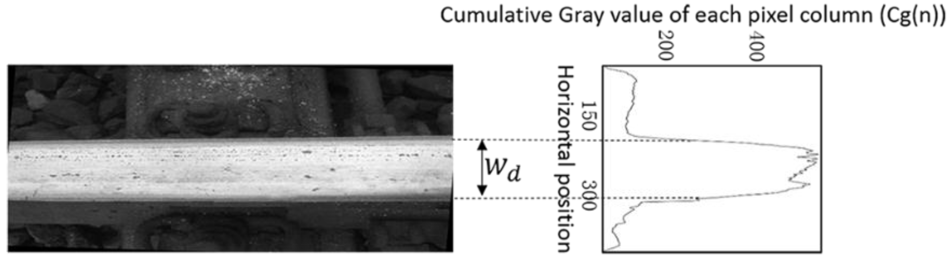
2.1. Rail Track Extraction

The rail images captured by UAVs involves redundant areas, as shown in Figure 3. Besides the areas of rail tracks, the rest areas are excluded for the next step. Therefore, Hough Transform and the method based on cumulative gray value of each pixel column are used to extract the area of rail track from rail images. Hough transform is a graphic detection algorithm based on the duality of point and line, and can be applied in the extraction of rail tracks [41].
Considering an image as a M × N matrix, the N-dimensional matrix C g that consists of cumulative gray value of each pixel column of the image matrix is determined by:
C g = [ i = 0 M 1 D i 0 , i = 0 M 1 D i 1 , i = 0 M 1 D i ( N 1 ) ] , C g ( n ) = i = 0 M 1 D i n ,    n [ 0 , N 1 ]
where, D x y is the pixel value of the coordinate (x, y). The matrix C g of the vertical rail image ( M = 550, N = 350) is shown in Figure 3. It should be noted that C g ( n ) is mapped to a small range. From this figure, it can be observed that the value C g ( n ) of area of the rail track is higher than the rest. This method is based on two factors: (1) Area of rail track has a higher value of C g ( n ) . (2) The width w d of the rail track is fixed in the rail image, as shown in Figure 3. The detail procedure about the method for rail track extraction is shown in Appendix A.

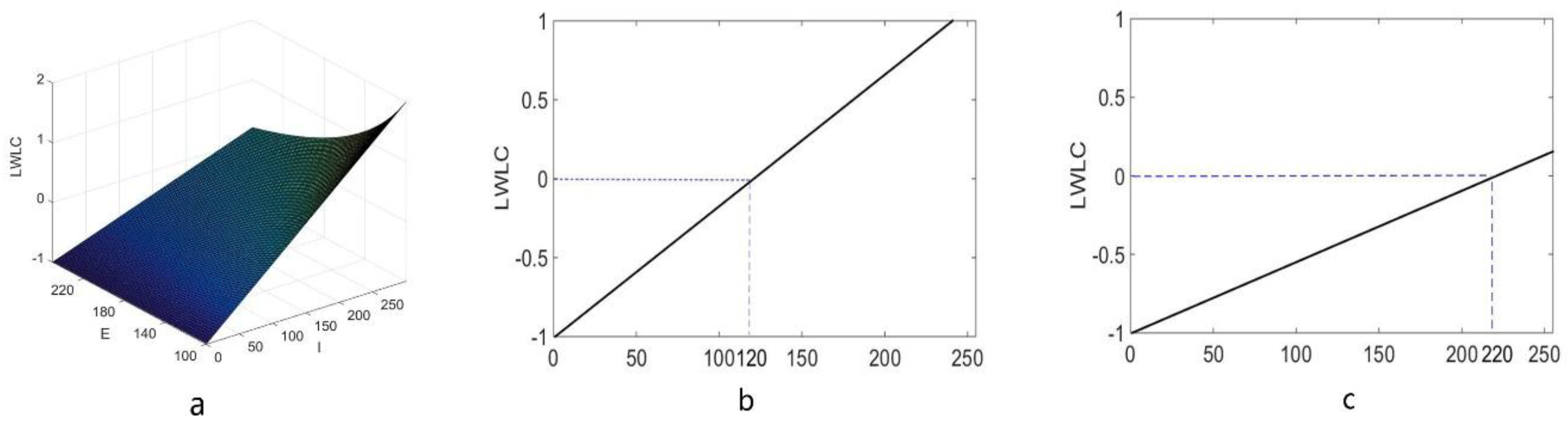
2.2. The Local Weber-Like Contrast Algorithm for Rail Images Enhancement

The brightness of images is non-uniform because of uneven natural light, the reflectance properties of rail surfaces [42], vibration of UAVs, or any other environmental factors. Therefore, defects and backgrounds are always mixed together. According to our experience, the following characteristics of UAV rail images occur:
  • Lower variation range of gray values in local regions. The reflection property and illumination of each longitudinal line in rail images is stable [14]. In the local line window, the variation range of gray values has small variation, and the most obvious features can be used for image enhancement [15].
  • Greater variation range of gray values in global scope. In general, the rail images have a large variation range of gray level in global scope due to uneven natural light and the reflectance properties of rail surfaces. The reflected light in smooth parts of rail surfaces is more than the rough parts [42].
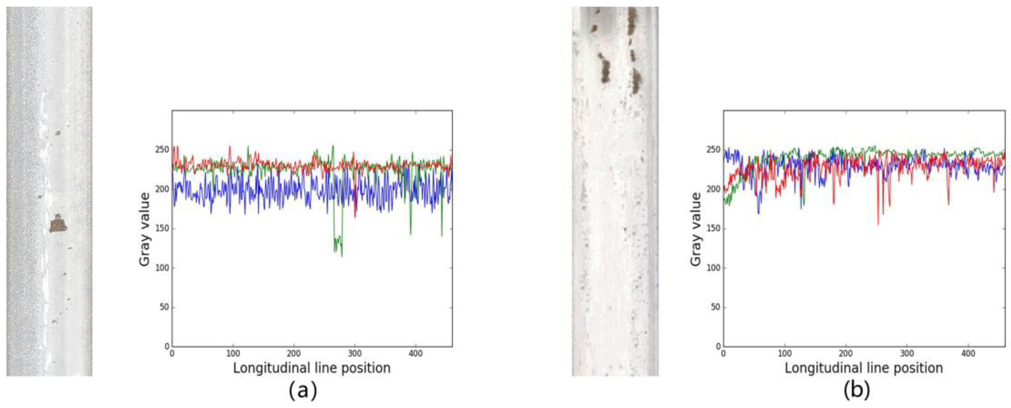
  • Confused gray values between defects and background. In general, the gray value of surface defects is lower than that of background, but the order is often broken because of illumination non-uniformity and noise corruption, as shown in the Figure 4.
  • Consistent features in the same longitudinal direction. Actually, a rail surface shares consistent features in the longitudinal direction as a train runs on a rail, since the friction for the points in the longitudinal direction between the rail surface and train wheels has an almost identical impact on the rail surface. In a rail image, intensity for the pixel points along longitudinal direction is consistent with relatively gray value changes caused by defect points and noise points [15]. Therefore, the surface discrete defects can be derived by the analysis of the information in longitudinal regions.
  • Higher gray mean of each longitudinal line for a track. According to our observation, the gray means along longitudinal lines of a UAV rail image are higher under normal conditions. This is because that UAV are supposed to fly in fine weathers and natural light conditions, and the surface reflectivity of rail tracks in operation is high because of its smoothness, as shown in the Figure 4.
As Figure 4 shows, the gray means along longitudinal lines of the image is high and the brightness of defects is quite low [14]. Since there are few defects in the image [30], the mean can be considered as background in the longitudinal direction. This feature completely satisfies a suitable range of Weber Contrast. As one of the most classical luminance contrast statistics, Weber Contrast is popular to cope with small, sharp-edged graphic objects on larger uniform backgrounds [43]:
C w = L o L b L b
where, L o is the luminance of the symbol and L b is the luminance of the immediately adjacent background. When the background is lighter than the object, C w is negative and ranges from 0 to −1. When the background is darker, C w is positive and ranges from 0 to potentially very large numbers.
Inspired by Weber Contrast and based on these characteristics for UAV rail images, the LWLC algorithm is proposed for adapting to different sunlight illuminance and eliminating the significant changes of gray-scale in this paper. The proposed gray stretch method for defects segmentation will be introduced in the next section. Assuming a pixel ( x , y ) and its surrounding window T in a rail image I, the intensity L W L C ( x , y ) of each pixel is given by:
L W L C ( x , y ) = I ( x , y ) E ( I ( x ˜ , y ˜ ) ) E ( I ( x ˜ , y ˜ ) ) ,    ( x ˜ , y ˜ ) T
where, I ( x , y ) denotes the gray value of the pixels in the image, E is the mean of I ( x ˜ , y ˜ ) in T in window T. Figure 5a shows LWLC value with the mean range [100, 255] due to higher brightness of UAV rail images. And Figure 5b,c present the curve with E = 100 and the curve with E = 220, respectively. In Figure 5b, the low range [0, 100] of I maps to [−1, 0], while the high range [100, 255] of I maps to (0, 155/100). In contrast, the curve with E = 220 in Figure 5c shows that the greater low range [0, 220] of I maps to [−1, 0] due to its low slope. Thereby, along with the brightness increasing, the LWLC value is progressively reduced and the stretch of the range of I is weakened. These characteristics are similar to the human vision system, that is likely to discern contrast under the darker illuminance [30,44].
The gray value I ( x , y ) of the pixels in an image can be approximately determined by:
I ( x , y ) = L ( x , y ) × R ( x , y )
where L ( x , y ) is light source intensity on the camera lens, and R ( x , y ) is the coefficient of reflection attribute [45]. In a local window T , L ( x , y ) can be regarded as a constant L due to the fact that the sunlight intensity in this small T reflected by the surface of a rail track is barely change under sunlight illumination. Therefore, Equation (3) can be replaced by:
L W L C ( x , y ) = L × R ( x , y ) L × μ ¯ R ( x ˜ , y ˜ ) L × μ R ¯ ( x ˜ , y ˜ ) = R ( x , y ) μ ¯ R ( x ˜ , y ˜ ) μ ¯ R ( x ˜ , y ˜ )       ,    ( x ˜ , y ˜ ) T
where μ R ¯ ( x ˜ , y ˜ ) is the mean of reflection attribute coefficient R ( x , y ) in a local window T . From this Equation (5), L W L C is just dependent on R ( x , y ) and μ R ¯ ( x ˜ , y ˜ ) rather than light source intensity L ( x , y ) . As a result, it is supposed that L W L C can keep steady under the change of sunlight illuminance. On the other hand, R ( x , y ) generally varies less in a local window T . This means that the value of R ( x , y ) μ ¯ R ( x ˜ , y ˜ ) approximates 0. Thereby, when there are a smooth background window T 1 with a large μ R ¯ ( x ˜ , y ˜ ) and a coarse background window T 1 with a small μ R ¯ ( x ˜ , y ˜ ) in a rail image, the difference of their L W L C matrix is not obvious. Therefore, a uniform background can be achieved by L W L C .
Briefly, rail surface defects and backgrounds can be highlighted and homogenized by L W L C . Based on these features, L W L C can enhance the UAV-based rail images of non-uniformity brightness due to the various reflection attribute of rail surfaces under various sunlight intensity.
A transformed image can be obtained by Equation (3), which has contrast enhancement. The choice of window T size is very important, because it affects the quality and efficiency of this algorithm. Based on UAV rail image features in the same longitudinal direction presented in the above characteristics, this study adopted a lined (longitudinal direction) window T (100 × 1) in this paper. The experiment in [30] also proves the excellent performance of this local line window.
In a local line window, gray value of defects is considered to be lower than the other areas on rail surface, because the light of the window is equal and less light can be reflected by defects. Therefore, if gray value of a pixel is lower than the mean value of all pixels in this window, it may be regarded as a defect point. In contrast, this is regarded as a background point. Based on these factors and Equation (3), the pixels belonging to non-defect (background and irregular) points can be translated into uniform background by setting a dynamic threshold E ( I ( x ˜ , y ˜ ) ) by
L W L C ( x , y ) = { I ( x , y ) E ( I ( x ˜ , y ˜ ) ) E ( I ( x ˜ , y ˜ ) ) ,     i f I ( x , y ) < E ( I ( x ˜ , y ˜ ) ) 0 ,        o t h e r w i s e .
In summary, the proposed LWLC algorithm for image enhancement is described as follows:
(i)
By convolution with an image matrix I and a designed lined window, calculates LWLC value of each pixel in I by Equation (6), so that a LWLC matrix can be acquired.
(ii)
Mapping gray-values of the LWLC matrix to [0, 255].

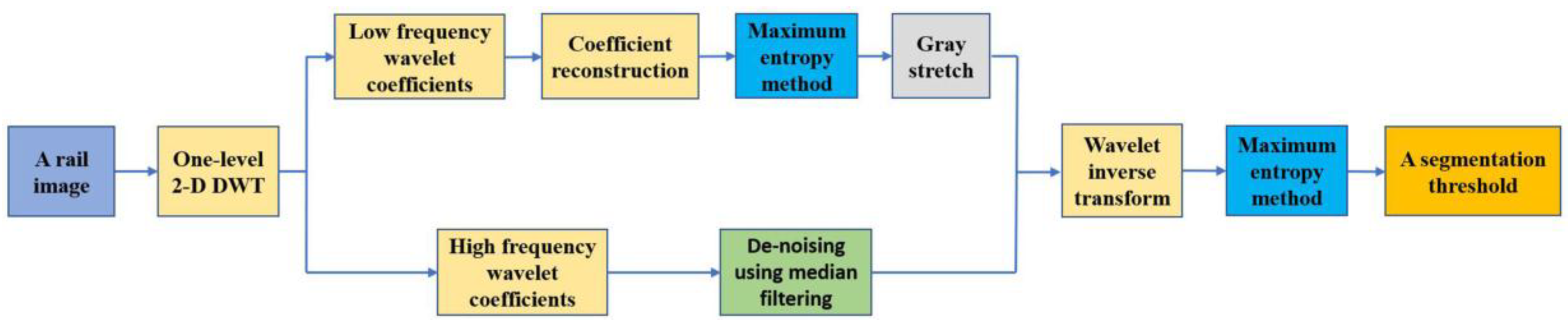
2.3. Defect Segmentation Mehtod Based on Gray Stretch Maximum Entropy

The GSME algorithm is able to determine an optimal segmentation threshold by stretching gray levels between the objection and background and reduces noise in the image’s wavelet domain. The procedure of the algorithm is shown in Figure 6.
Based on one-level 2-D DWT algorithm, the rail image is decomposed into four bands (LL, HL, LH, HH). For the LL band, the ME algorithm is used to obtain a segmentation threshold after reconstructing its coefficient, and then the gray stretch method is used to enhance contrast between background and foreground. For HL, LH and HH bands, the median filtering template of horizontal line, vertical line, and diagonal line is used to eliminate noise of three high frequency wavelet coefficients, respectively.
Subsequently, the ME algorithm is used to select a segmentation threshold after reconstructing the rail image.

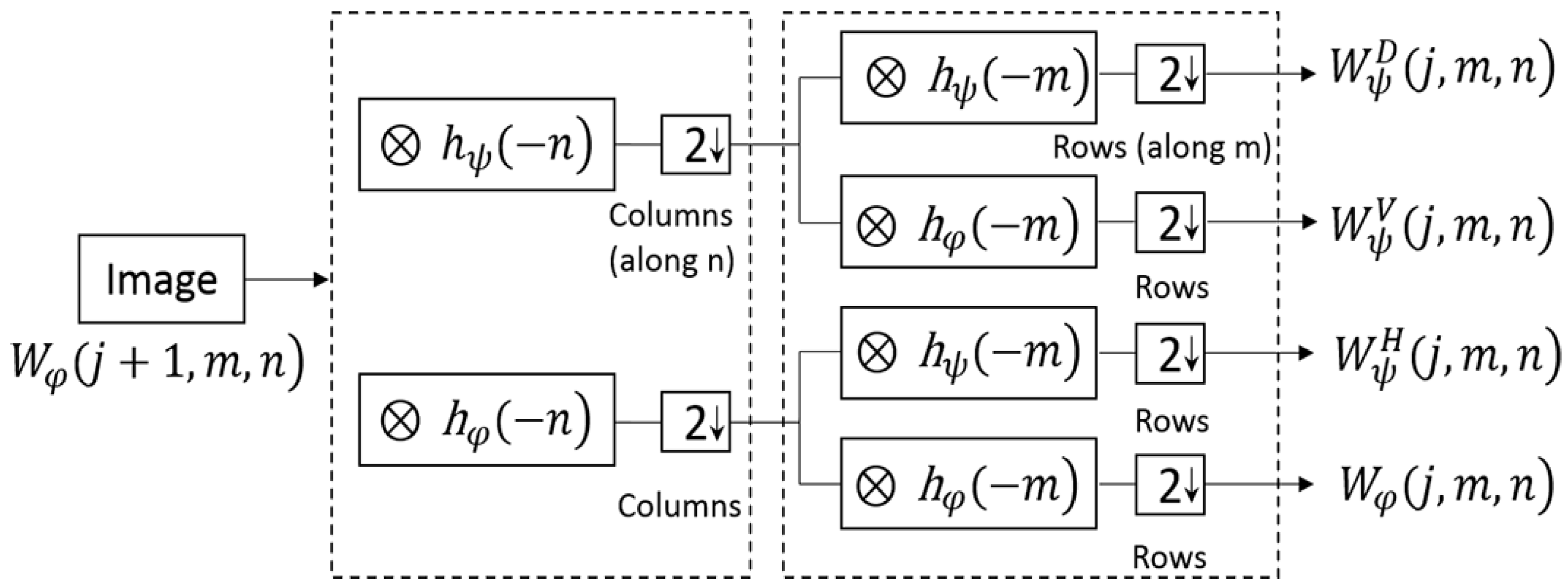
2.3.1. A Brief Introduction for 2-D Discrete Wavelet Transform

The discrete wavelet transform (DWT) can not only express some features of a signal easily and efficiently, but also provides a powerful insight into an image’s spatial and frequency characteristics [38,46]. Two-dimensional functions such as images can be expanded from one-dimensional wavelet transform [46]. In two dimensions, a 2-D scaling function and three 2-D wavelets are given by:
φ ( x , y ) = φ ( x ) φ ( y ) ψ H ( x , y ) = ψ ( x ) φ ( y ) ψ V ( x , y ) = φ ( x ) ψ ( y ) ψ D ( x , y ) = ψ ( x ) ψ ( y )
where φ ( x , y ) is a two-dimensional scaling function, ψ H corresponds to some variations along columns(such as horizontal edges), ψ V corresponds to variations along rows (for example, vertical edges), and ψ D responds to variations along diagonals. Each of them can be seen as products of two 1-D functions. If the 2-D scaling and wavelets functions are given, the 1-D DWT can be extended to two dimensions. Firstly, the scaled and translated basis functions are defined as:
φ j , m , n ( x , y ) = 2 j 2 φ ( 2 j x m ,    2 j y n )
ψ i j , m , n ( x , y ) = 2 j 2 ψ ( 2 j x m ,    2 j y n ) ,     i = { H , V , D }
where index i is a superscript that assumes the values H, V, and D in Equation (7). The discrete wavelet transform of M × N image f ( x , y ) is given by:
W φ ( j 0 , m , n ) = 1 M N x = 0 M 1 y = 0 N 1 f ( x , y ) φ j 0 , m , n ( x , y )
W ψ i ( j , m , n ) = 1 M N x = 0 M 1 y = 0 N 1 f ( x , y ) ψ j , m , n i ( x , y ) ,        i = { H , V , D }
where j 0 is an arbitrary starting scale that is set to 0 by default, the W φ ( j 0 , m , n ) coefficients are an approximation of f ( x , y ) at scale j 0 , and the W ψ i ( j , m , n ) coefficients add horizontal, vertical, and diagonal details for scales j j 0 . The 2-D DWT is achieved by using digital filters and down-sampling, as shown in Figure 7. According to the 2-D DWT scaling and wavelet functions, we can take the 1-D FWT (fast wavelet transform) of the rows of f ( x , y ) , followed by the 1-D FWT of the resulting columns. Therefore, an original 2-D image can be decomposed into four sub-image sets which contain different frequency characteristics by high-pass and low-pass filter: a scaling component W φ involving low-pass information and three wavelet components, W ψ H , W ψ D , and W ψ V , corresponding respectively to the horizontal, diagonal, and vertical details, as in Figure 5. The 1-level DWT method can also reduce noise and the background disturbances.

2.3.2. The Gray Stretch Maximum Entropy Threshold Method

T. Pun et al. proposed the entropy threshold principle [47,48] which uses entropy of image gray histogram to obtain the segmentation threshold. The maximum entropy (ME) algorithm [37] is proposed to optimize a threshold afterwards. ME method can confirm one threshold which maximizes the total content of information provided by cumulative object probability distribution ϕ o and cumulative background probability distribution ϕ b . They are given by:
P n = f n M ,    n [ 0 , 255 ]
ϕ o = n = 0 T 1 p n , ϕ b = 1 ϕ o
where P n is the probability of gray value n in an image. Given a rail image I that is normalized to 256 gray levels, and the entropy of ϕ o and ϕ b is defined as:
H o ( T ) = n = 0 T 1 ( P n ϕ o ( T ) ln P n ϕ o ( T ) ) ,
H b ( T ) = n = T 255 ( P n ϕ b ( T ) ln P n ϕ b ( T ) )
where M is the total pixel number of image I, f n is the frequency of gray value n in I . An optimal threshold T* can be obtained by:
T * = arg    max    ( H o ( T ) + H b ( T ) ) ,     T [ 0 , 255 ]
The ME method takes into account both the distribution information of image pixel gray and the spatial information of pixels. However, its performance is not perfect for defect segmentation due to the aforementioned characteristics of rail images. Therefore, GSME algorithm is proposed in this paper, as shown in Figure 6.
(i)
Based on one-level 2-D DWT algorithm, the rail image is decomposed into four wavelet coefficients that include approximation (low frequency region), horizontal, vertical, and diagonal details.
(ii)
For low frequency region (LL region) of image decomposed by wavelet, the ME algorithm is used to obtain a segmentation threshold after reconstructing its coefficient, and then the gray stretch method is used to enhance contrast between background and foreground, as the following equations:
f φ ( x , y )    =    1 M N m n W φ ( j 0 , m , n ) φ j 0 , m , n ( x , y ) ,
f φ * ( x , y ) = { f φ ( x , y ) a f φ ( x , y ) ,     i f     f φ ( x , y ) < T * f φ ( x , y ) + a f φ ( x , y ) ,          o t h e r w i s e .
where f φ ( x , y )    denotes reconstructing image function, a denotes stretch factor and is set to and value between 0.1 and 0.5 in general.
(iii)
For the image, its energy is mainly distributed in the low frequency region. In the high frequency area, the proportion of noise energy is large, so this study focuses on de-noising in this area. In Ref [39], Tang et al. use the filter templates of three different directions for de-noising. For example, the line template of horizontal direction is used for W ψ H de-noising, because the wavelet coefficients contain the high-frequency information in the horizontal direction and low-frequency information in the vertical direction of the image signal. Inspired by the median filtering method employed in wavelet domain, this study used the median filtering template of horizontal line, vertical line, and diagonal line to eliminate noise of three high frequency wavelet coefficients, respectively.
(iv)
The rail image can be reconstructed based on discrete wavelet inverse transform algorithm. The formula for reconstruction image is given by:
f ( x , y ) =    f φ * ( x , y ) + 1 M N i = H , V , D j = j 0 m n W ψ i ( j , m , n ) ψ j , m , n i ( x , y )
(v)
The ME algorithm is used to select a segmentation threshold after reconstructing the rail image by discrete wavelet inverse transform.
The GSME algorithm performs well for processing rail images in which the contrast between foreground and background is low.

3. Experiment Results

To demonstrate the proposed LWLC-GSME model, experiments were carried out with comparisons with related well-established methods.

3.1. Experiment Setup

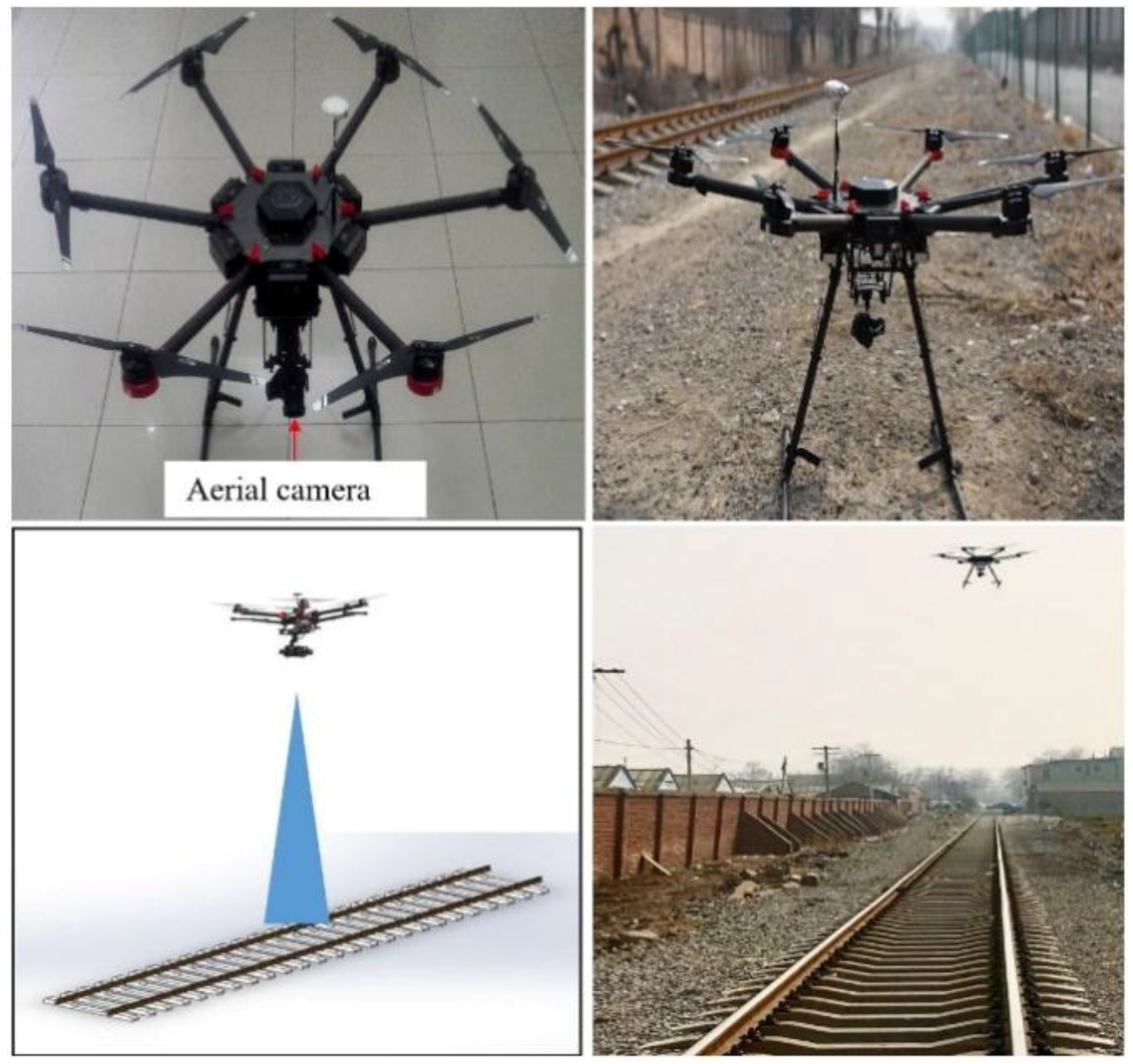
3.1.1. A Brief Introduction of the Equipment for UAV Images Acquisition

As shown in Figure 6, the DJI Matrice 600 equipped with Zenmuse Z30 (DJI-Innovations, Shenzhen, China) was used to capture rail images. The Matrice 600 is a six-rotor flying platform designed for professional aerial photography and industrial applications. The aircraft uses six Intelligent Flight Batteries to extend the time of flight. The built-in API Control feature, expandable center frame, and maximum takeoff weight of 15.1 kg make the Matrice 600 ideal for connecting other devices to meet the specific needs of different applications. The Zenmuse Z30 enables non-contact distance detection by a high-performance camera system with a zoom lens. This aerial camera offers 30× optical zoom, 6× digital zoom, and HD 1080P video. The UAV adopts an industrial level Zenmuse platform with a precision of 0.01 degrees, so the problem of image blur caused by jitter is effectively solved.

3.1.2. Experiment Environment

As shown in Figure 8, the UAV equipped with an aerial camera was used to capture image or video information of rails as it flies overhead. Then, customized image processing software was used to analyze the captured UAV images. To avoid interference of obstructions, the flight height was set to 30 m. The images of rail tracks from the UAV were acquired on the freight line near the Baoding railway south station and the freight line near Nansihuan in Beijing. One of the experiment environments is shown in Figure 7. The speed of the UAV and the actual length of the rail track in an UAV image are 2 m/s and 1 m, respectively. Therefore, to cover every part of the rail tracks, the frequency of the camera shutter is set to 2 frames per second. Each image captured by an UAV has corresponding POS information that contains the coordinates of the aircraft at that moment, and therefore, the location of rail defects can be found based on these coordinates.

3.1.3. Defects and Evaluation

All images used for this experiment were captured, and several examples of UAV images containing discrete defects are shown in Figure 9. A large dataset was constructed to verify the algorithm, which contains 50 rail images, and each one has a lot of defects (more than 2) on its surface. Rail surface defects are divided into two categories depending on size and maintenance standard of the railway. In general, a defect whose size is larger than 255 mm2 should be inspected as soon as possible, because it may result in serious accidents [49]. Therefore, in our data set, the defects are divided into two types, according to size Ω of defects, as shown in Table 1.
The dataset includes 208 defects: 126 in T-I and 82 in T-II. These defects are labeled by experts.
Within the Matlab 2014 compile environment, the designed software is achieved by Matlab program languages, and an inspected defect is automatically marked by a rectangle. Then, the inspected defect is accepted as correct if it matches the marked defect in the corresponding image.
In information retrieval and pattern recognition, recall and precision are the basic criteria for evaluation of retrieval quality. The two criteria are used for evaluation of our experiment result in this paper. The precision (P) and recall (R) are respectively given by:
P = TP/(TP + FP)
R = TP/NP
where TP is the number of defects that were inspected correctly, FP is the number of wrongly inspected defects, and NP is the number of marked defects for the corresponding defect category (T-I and T-II). Specifically, the recall is more significant than precision, because a defect which is not detected may have severe consequences.
It should be noted that each defect in the dataset is labeled with a minimum enclosing rectangle; thereby, the real region of rail surface defects is approximated by the region of its minimum enclosing rectangle. As to the LWLC-GSME model, all these detected defects are also automatically marked by a minimum enclosing rectangle. This is regard as correct inspection if the minimum enclosing rectangle of a detected defect overlaps the corresponding labeled image more than 85%; otherwise, it is error detection. TP denotes number of defects that were correctly inspected.

3.2. Performance Analysis

Two groups of visual comparison experiments and a qualitative comparison experiment for defects inspection are presented in this section. Every defect in the images is marked by a red rectangle.

3.2.1. Image Enhancement

The effectiveness of image enhancement method was first verified by performing experiments on several randomly selected images. It should be noted that these selected images include defects for types T-I and T-II, and have characteristics of low contrast and varying illumination. In this section, this paper compares the LWLC algorithm with traditional enhancement methods, including histogram equalization (HE), LN [14] and MLC [30] algorithms.
Figure 10 presents comparison results of these methods. The HE method only averages the gray level distribution rather than enlarging the gray scale, and retains a number of irregular (noise) points, as shown in the Figure 10B. The LN method has poor enhancement effect because the image loses a lot of the significant detailed information. Not surprisingly, the MLC algorithm achieves competitive performance and highlights defects on UAV-based rail images. However, to UAV-based rail images having high brightness mean and a great deal irregular points, the MLC algorithm has a poor ability at extending grayscale range between irregular points and defect points. The MLC algorithm can distinguish defects from background, but the distinguishing capability for irregular (noise) points and defect points is not as good as that of the LWLC algorithm. As shown in Figure 10D,E, the enhanced defects by LWLC algorithm are more obviously highlighted than the MLC algorithm.
It is worth noting that the proposed method can effectively remove the influence of uneven illumination. As shown in Figure 10A, for the above two images with several shadows, the global image enhancement method (HE method, as shown in Figure 10B) makes images loss detail information and amplifies irregular points (noise points and shadow points), since the HE is a linear algorithm and only averages the gray level distribution. In addition, although the LN method (as shown in Figure 10C) can remove shadows, it also removes defects, due to the fact that a rail surface contains a small number of defects, and the difference between defects and backgrounds in longitudinal direction is large. However, because of few defects existing on rail surfaces and high reflection properties of rail surfaces, the brightness mean of longitudinal line along a track approximates to the background luminance. Thereby, the proposed LWLC algorithm based on Weber’s law can address these issues, and effectively remove the uneven illumination due to the feature of Weber’s law presented in Section 1. It can be seen that the proposed LWLC algorithm is superior to other two methods, as shown in the Figure 10E.
For defect segmentation, the LWLC algorithm combined with the GSME method can achieve better performance, and the experiment of defect segmentation will be described in the next section.

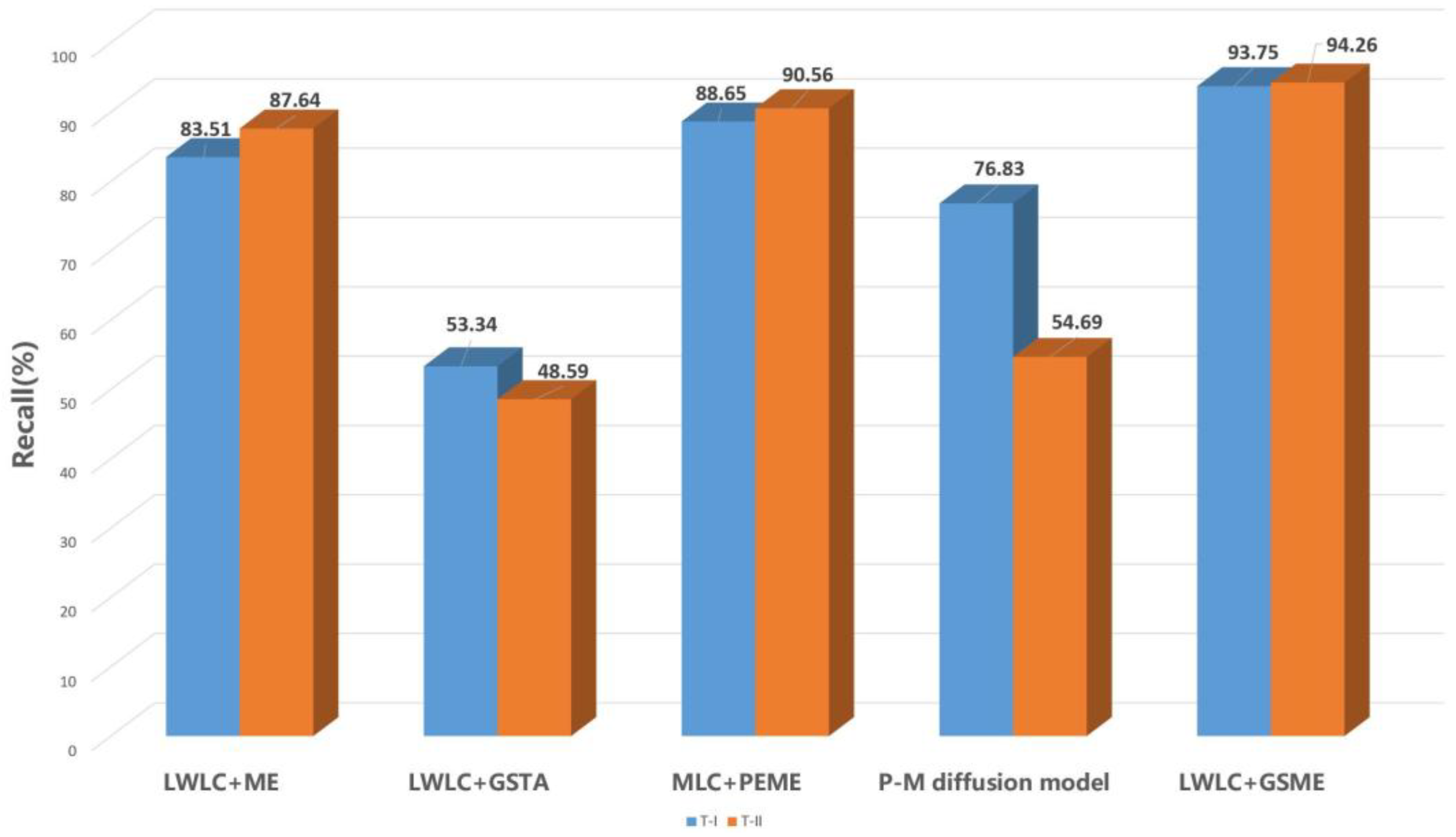
3.2.2. Defect Segmentation

On the basis of the LWLC, this paper compares GSME with traditional image segmentation methods including the maximum entropy (ME) algorithm, the proportion emphasized maximum entropy (PEME) algorithm, and the GSTA method. The ME [37] method can confirm one threshold which maximizes the total content of information provided by object distribution and background distribution. After enhancing images by MLC, PEME [30] is used to obtain an optimal segmentation threshold. PEME is an improved ME method which reduces the proportion of the background information and increases an exponent factor in original equation. The GSTA method uses wavelet transform and the Otsu algorithm to enhance image edges, then Otsu to extract the objection of the image. In the comparative experiment, the PEME method adopts MLC for image enhancement, and the other three adopt the same LWLC approach. All methods adopt the same evaluation criterion mentioned above, as shown in Figure 11. According to the Refs. [30,38] and our experiment, the parameter ρ of GSTA method, the parameter β of MLC+PEME and the parameter α of LWLC+GSME are set to 0.2, 2, and 0.3, respectively.
As shown in Figure 11B, LWLC+ME can retain more detailed information of defects than the LWLC+GSTA and MLC+PEME methods, but its performance in terms of noise suppression, non-defect points removal, and defect details preservation is weaker than that of LWLC+GSME. Reasons for the inapplicability of the PEME approach are as follows: on one hand, UAV images have lower contrast, relatively obscure texture features, and more noise due to lighting based on natural light and higher distance between camera and rail; on the other, the variation in natural illumination can’t be controlled by a human being, and it has an inevitable effect on defect extraction. If the image is captured as the aircraft flies above the rail at different distances, there is no uniform model to set the exponent factor β of the PEME model. In Figure 11C, it can be seen that defect details including shape and area information can’t be effectively retained by the LWLC+GSTA method, and there are more noise and non-defect points than with the other methods. Figure 11D shows that MLC+PEME highlighted defect areas, but that noise and non-defect points in the image can’t be restrained. As shown in Figure 11E, it can be seen that defects are remarkably segmented with the least noise and non-defect points based on LWLC+GSME.

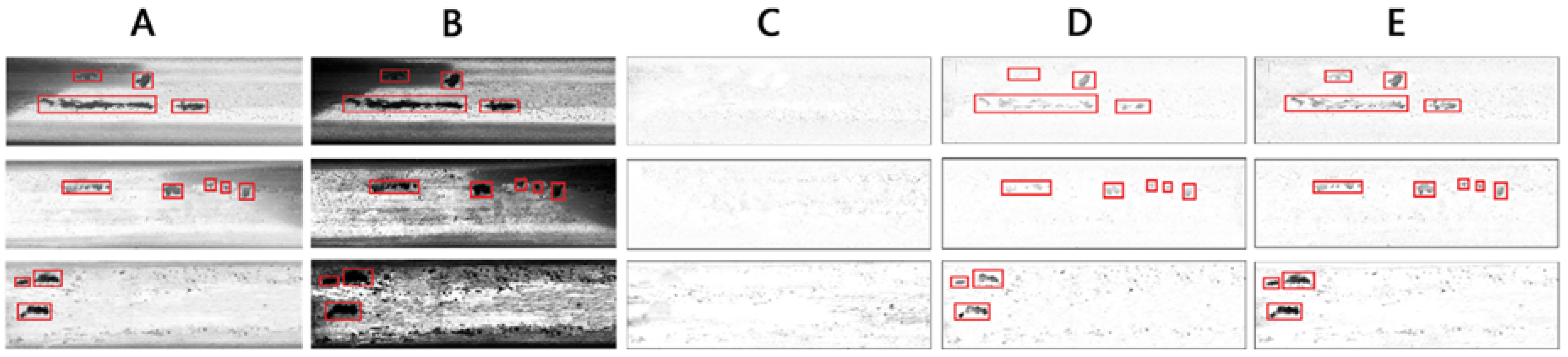
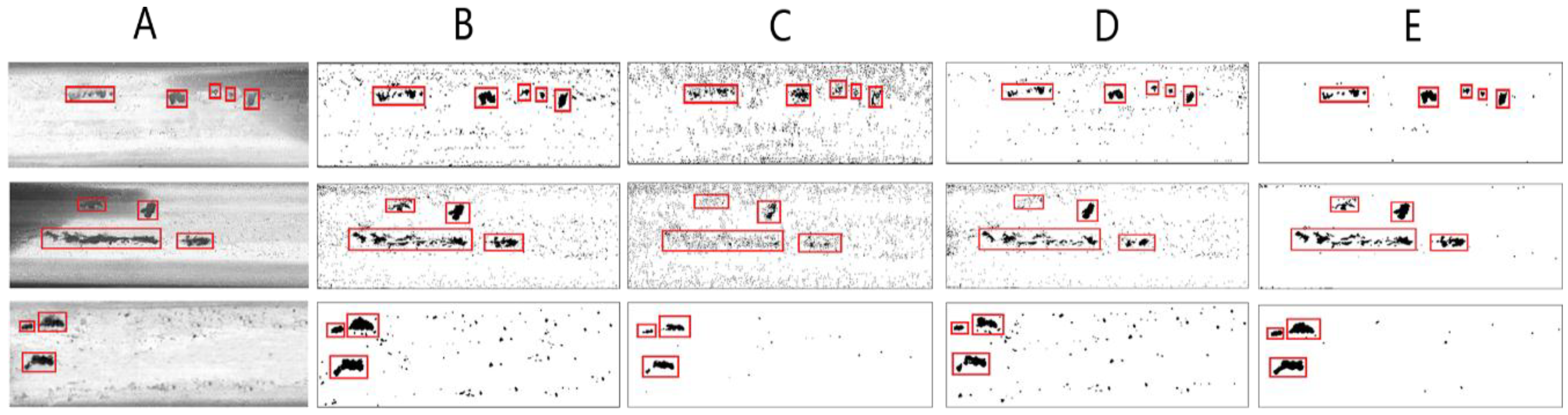
3.2.3. Qualitative Comparison between LWLC+GSME and Related Methods

Finally, a quantitative analysis for the defect inspection after segmentation is given by Figure 12 and Figure 13. The two figures further explain that the LWLC+GSME method is more suitable for detection of rail defects based on the UAV image.
Although the GSTA method enhances image contrast, it can’t repress interference of noise effectively. These three methods acquire poor segmentation effects because they are susceptible to noise and background points. In contrast, LWLC+GSME not only achieves contrast enhancement between defects and background, but also obtains the best segmentation effects. For example, LWLC+GSME achieves a precision of 88.63% for T-I defects and a precision of 90.32% for T-II defects. It should be noted that both of MLC+PEME and LWLC+GSME obtain similar effects for precision, because they see non-defect regions as defect under light disturbance (such as uniform illumination and low contrast).
In addition, based on the ME principle and characteristics of the defects mentioned above, a suitable segmentation threshold should be relatively small under the condition of complete retention of defects [30]. Three examples of the segmentation threshold with four segmentation methods are shown in Table 2. From this table, a relatively small threshold is obtained based on LWLC+GSME. It further illustrates that the proposed method can select a better segmentation threshold. It should be noted that thresholds based on LWLC+GSTA are the smallest. However, this method achieves poor performance for T-I and T-II defects, as shown in Figure 11 and Figure 12; this is because this method uses Gaussian kernels to enhance object edges of high frequency areas in the wavelet domain, and UAV-based images contain a lot of irregular (noise) points. For this reason, the method also enhances these noises in rail images, thereby yielding poor defects detection performance.

4. Conclusions

To cope with rail surface defects, an inspection approach based on UAV images is proposed in this study. The proposed LWLC algorithm can highlight not only defects and homogenized backgrounds of UAV-based rail images, but also eliminates the adverse effects of non-uniform illumination. Furthermore, we put forward the GSME method for defects segmentation, which reduces irregular points and obtains excellent segmentation effects. The integrated LWLC+GSME method further illustrates great flexibility and effectiveness in detecting discrete defects.
Finally, this study compared LWLC and LWLC+GSME with related methods, and the results of experiments show the significance of the proposed method. The quantitative experimental results show that the proposed method achieves a recall of 93.75% for T-I defects and of 94.26% for T-II defects, and that it is efficient and feasible to detect rail surface defects based on UAV images. It was verified that the proposed model can obtain excellent results.
In future, our research work will focus on the following two aspects: firstly, we will explore new models for rail defect classification based on UAV images and assess the health of rails; secondly, based on the development of high UAV photography, fast detection models in complex environments will be developed to increase detection efficiency.

Author Contributions

Y.W. collected and analyzed the data, made charts and diagrams, conceived and performed the experiments and wrote the paper; Y.Q. conceived the structure and provided guidance; Z.W. provided the UAV equipment and searched the literature; L.J. modified the manuscript.

Funding

This research is supported by the National Key R&D Program of China (No. 2016YFB1200203), National Natural Science Foundation of China (No. 91738303) and State Key Laboratory of Rail Traffic Control and Safety (Contract Nos. RCS2016ZQ003 and RCS2016ZT018)

Acknowledgments

This research is also supported by National Engineering Laboratory for System Safety and Operation Assurance of Urban Rail Transit.

Conflicts of Interest

The authors declare no conflict of interest.

Appendix A

In order to reduce the computation payload, the colored image is transformed into a gray image. The method for rail track extraction is described as follows.
Firstly, the longest line of rail edge is detected by Hough transform, as shown in Figure A1B, and the image is rotated by the angle ϴ between the line and horizontal direction so that the rails are parallel to the vertical direction, as shown in Figure A1C. And then the followed Algorithm A1 is used to find the most left position of a rail track after the matrix Cg(n) is obtained by Equation (1).
Algorithm A1. The Algorithm A1 for track extraction.
1  procedure Algorithm A1 (Cg(n), Wd)
2  for m ← 1, MWd + 1 do
3    for nm, Wd do  /* Wd is the width of the rail track.*/
4      Cg(n) ← Cg(n) + Cg(n + 1)
5    CumCg(m) ← Cg(n)
6  end for
7  maxCumCg ← −1
8  p_left ← 0
9  for m ← 1, MWd + 1 do
10    p_CumCg ← CumCg(m)
11    if p_CumCg > maxCumCg then
12     maxCumCgp_CumCg
13     p_left ← m
14    end if
15  end for
16  return p_left   /* The most left position of a rail track (p_left)*/
17  end procedure
Figure A1. The example of the rail track extraction. (A) The original image contains a rail. (B) The detection for the longest line and the inclined angle ϴ of the rail based on Hough transform method. (C) The rail image correction by rotating the angle ϴ. (D) The rail track extraction based on integral projection of vertical pixel column for a rail image.
Applsci 08 01028 g0a1

References

  1. Arivazhagan, S.; Shebiah, R.N.; Magdalene, J.S.; Sushmitha, G. Railway track derailment inspection system using segmentation based fractal texture analysis. ICTACT J. Image Video Process. 2015, 6, 1060–1065. [Google Scholar]
  2. Cannon, D.; Edel, K.O.; Grassie, S.; Sawley, K. Rail defects: An overview. Fatigue Fract. Eng. Mater. Struct. 2003, 26, 865–886. [Google Scholar] [CrossRef]
  3. Grassie, S. Rail corrugation: Characteristics, causes, and treatments. Proc. Inst. Mech. Eng. Part F J. Rail Rapid Transit 2009, 223, 581–596. [Google Scholar] [CrossRef]
  4. Edwards, J.R.; Hart, J.M.; Sawadisavi, S.; Resendiz, E.; Barkan, C.; Ahuja, N. Advancements in Railroad Track Inspection Using Machine-Vision Technology. In Proceedings of the AREMA Conference on American Railway and Maintenance of Way Association, Chicago, IL, USA, 2–5 August 2009. [Google Scholar]
  5. Marino, F.; Distante, A.; Mazzeo, P.L.; Stella, E. A real-time visual inspection system for railway maintenance: Automatic hexagonal-headed bolts detection. IEEE Trans. Syst. Man Cybern. Part. C (Appl. Rev.) 2007, 37, 418–428. [Google Scholar] [CrossRef]
  6. Tsai, D.-M.; Wu, S.-C.; Chiu, W.-Y. Defect detection in solar modules using ICA basis images. IEEE Trans. Ind. Inform. 2013, 9, 122–131. [Google Scholar] [CrossRef]
  7. Zhang, X.; Feng, N.; Wang, Y.; Shen, Y. An analysis of the simulated acoustic emission sources with different propagation distances, types and depths for rail defect detection. Appl. Acoust. 2014, 86, 80–88. [Google Scholar] [CrossRef]
  8. Liu, Z.; Li, W.; Xue, F.; Xiafang, J.; Bu, B.; Yi, Z. Electromagnetic tomography rail defect inspection. IEEE Trans. Magn. 2015, 51, 1–7. [Google Scholar] [CrossRef]
  9. Hesse, D.; Cawley, P. The Potential of Ultrasonic Surface Waves for Rail Inspection. In Proceedings of the AIP Conference, Golden, CO, USA, 25–30 July 2004; American Institute of Physics: College Park, MD, USA, 2005; Volume 760, pp. 227–234. [Google Scholar]
  10. Tang, X.-N.; Wang, Y.-N. Visual inspection and classification algorithm of rail surface defect. Comput. Eng. 2013, 9, 25–30. [Google Scholar]
  11. Resendiz, E.; Hart, J.M.; Ahuja, N. Automated visual inspection of railroad tracks. IEEE Trans. Intell. Transp. Syst. 2013, 14, 751–760. [Google Scholar] [CrossRef]
  12. Liu, J.; Li, B.; Xiong, Y.; He, B.; Li, L. Integrating the symmetry image and improved sparse representation for railway fastener classification and defect recognition. Math. Probl. Eng. 2015, 2015, 462528. [Google Scholar] [CrossRef]
  13. Ph Papaelias, M.; Roberts, C.; Davis, C. A review on non-destructive evaluation of rails: State-of-the-art and future development. Proc. Inst. Mech. Eng. Part F J. Rail Rapid Transit 2008, 222, 367–384. [Google Scholar] [CrossRef]
  14. Li, Q.; Ren, S. A real-time visual inspection system for discrete surface defects of rail heads. IEEE Trans. Instrum. Meas. 2012, 61, 2189–2199. [Google Scholar] [CrossRef]
  15. Gan, J.; Li, Q.; Wang, J.; Yu, H. A hierarchical extractor-based visual rail surface inspection system. IEEE Sensors J. 2017, 17, 7935–7944. [Google Scholar] [CrossRef]
  16. He, Z.; Wang, Y.; Yin, F.; Liu, J. Surface defect detection for high-speed rails using an inverse pm diffusion model. Sens. Rev. 2016, 36, 86–97. [Google Scholar] [CrossRef]
  17. Sieberth, T.; Wackrow, R.; Chandler, J.H. Automatic detection of blurred images in UAV image sets. ISPRS J. Photogramm. Remote Sens. 2016, 122, 1–16. [Google Scholar] [CrossRef] [Green Version]
  18. Siebert, S.; Teizer, J. Mobile 3d mapping for surveying earthwork projects using an unmanned aerial vehicle (UAV) system. Autom. Constr. 2014, 41, 1–14. [Google Scholar] [CrossRef]
  19. Pérez-Ortiz, M.; Peña, J.M.; Gutiérrez, P.A.; Torres-Sánchez, J.; Hervás-Martínez, C.; López-Granados, F. Selecting patterns and features for between-and within-crop-row weed mapping using UAV-imagery. Expert Syst. Appl. 2016, 47, 85–94. [Google Scholar] [CrossRef]
  20. Wang, L.; Zhang, Z. Automatic detection of wind turbine blade surface cracks based on UAV-taken images. IEEE Trans. Ind. Electron. 2017, 64, 7293–7303. [Google Scholar] [CrossRef]
  21. Liu, C.; Liu, Y.; Wu, H.; Dong, R. A safe flight approach of the UAV in the electrical line inspection. Int. J. Emerg. Electr. Power Syst. 2015, 16, 503–515. [Google Scholar] [CrossRef]
  22. Kaamin, M.; Idris, N.A.; Bukari, S.M.; Ali, Z.; Samion, N.; Ahmad, M.A. Visual Inspection of Historical Buildings Using Micro UAV. In Proceedings of the MATEC Web of Conferences, Qingdao, China, 25–27 August 2017; EDP Sciences: Paris, France, 2017; Volume 103, p. 07003. [Google Scholar]
  23. Yuan, C.; Liu, Z.; Zhang, Y. UAV-Based Forest Fire Detection and Tracking Using Image Processing Techniques. In Proceedings of the 2015 International Conference on Unmanned Aircraft Systems (ICUAS), Denver, CO, USA, 9–12 June 2015; pp. 639–643. [Google Scholar]
  24. Rau, J.; Hsiao, K.; Jhan, J.; Wang, S.; Fang, W.; Wang, J. Bridge crack detection using multi-rotary UAV and object-base image analysis. Int. Arch. Photogramm. Remote Sens. Spat. Inf. Sci. 2017, 42, 311. [Google Scholar] [CrossRef]
  25. Arenella, A.; Greco, A.; Saggese, A.; Vento, M. In Real Time Fault Detection in Photovoltaic Cells by Cameras on Drones. In Proceedings of the 14th International Conference on Image Analysis and Recognition, Montreal, QC, Canada, 5–7 July 2017; Springer: New York, NY, USA, 2017; pp. 617–625. [Google Scholar]
  26. Xiao, Q.; Zhang, Q.; Wu, X.; Han, X.; Li, R. Learning Binary Code Features for UAV Target Tracking. In Proceedings of the 3rd IEEE International Conference on Control Science and Systems Engineering (ICCSSE), Beijing, China, 17–19 August 2017; IEEE: Piscataway, NJ, USA, 2017; pp. 65–68. [Google Scholar]
  27. Baykara, H.C.; Bıyık, E.; Gül, G.; Onural, D.; Öztürk, A.S. Real-Time Detection, Tracking and Classification of Multiple Moving Objects in UAV Videos. In Proceedings of the 2017 IEEE 29th International Conference on Tools with Artificial Intelligence (ICTAI), Boston, MA, USA, 6–8 November 2017; IEEE: Piscataway, NJ, USA, 2017; pp. 945–950. [Google Scholar]
  28. Radovic, M.; Adarkwa, O.; Wang, Q. Object recognition in aerial images using convolutional neural networks. J. Imaging 2017, 3, 21. [Google Scholar] [CrossRef]
  29. Liang, L.; He, W.-P.; Lei, L.; Zhang, W.; Wang, H.-X. Survey on enhancement methods for non-uniform illumination image. Appl. Res. Comput. 2010, 5, 008. [Google Scholar]
  30. Li, Q.; Ren, S. A visual detection system for rail surface defects. IEEE Trans. Syst. Man Cybern. Part C (Appl. Rev.) 2012, 42, 1531–1542. [Google Scholar] [CrossRef]
  31. Chen, X.; Xu, J.-P. A denoising algorithm of image for UAV based on wavelet transform and mean-value filtering. Fire Control Command. Control 2011, 8, 049. [Google Scholar]
  32. Jin, X.; Wen, Z.; Wang, K. Effect of track irregularities on initiation and evolution of rail corrugation. J. Sound Vib. 2005, 285, 121–148. [Google Scholar] [CrossRef]
  33. Fechner, G. Über ein wichtiges psychophysiches grundgesetz und dessen beziehung zur schäzung der sterngrössen. Abk. K. Ges. Wissensch. Math.-Phys. K 1858, 1, 4. [Google Scholar]
  34. Shen, J. On the foundations of vision modeling: I. Weber’s law and Weberized TV restoration. Phys. D Nonlinear Phenom. 2003, 175, 241–251. [Google Scholar] [CrossRef]
  35. Available online: https://en.wikipedia.org/wiki/Contrast_(vision) (accessed on 1 May 2018).
  36. Otsu, N. A threshold selection method from gray-level histograms. IEEE Trans. Syst. Man Cybern. 1979, 9, 62–66. [Google Scholar] [CrossRef]
  37. Kapur, J.N.; Sahoo, P.K.; Wong, A.K. A new method for gray-level picture thresholding using the entropy of the histogram. Comput. Vis. Graph. Image Process. 1985, 29, 273–285. [Google Scholar] [CrossRef]
  38. Liu, L.; Yang, N.; Lan, J.; Li, J. Image segmentation based on gray stretch and threshold algorithm. Opt.-Int. J. Light Electron. Opt. 2015, 126, 626–629. [Google Scholar] [CrossRef]
  39. Tang, S.-W.; Lin, J. Image denoising with combination of wavelet transform and median filtering. J. Harbin Inst. Technol. 2002, 24, 1334–1336. [Google Scholar]
  40. Rakheja, P.; Vig, R. Image denoising using combination of median filtering and wavelet transform. Int. J. Comput. Appl. 2016, 141, 31–35. [Google Scholar] [CrossRef]
  41. Jin, B.; Niu, H.; Hou, T. Study of straight line rail image edge detection based on improved hough. Video Eng. 2015, 39, 17–19. [Google Scholar]
  42. Li, Q.; Tan, Y.; Huayan, Z.; Ren, S.; Dai, P.; Li, W. A Visual Inspection System for Rail Corrugation Based on Local Frequency Features. In Proceedings of the 2016 IEEE 14th International Conference on Dependable, Autonomic and Secure Computing, 14th International Conference on Pervasive Intelligence and Computing, 2nd International Conference on Big Data Intelligence and Computing and Cyber Science and Technology Congress (DASC/PiCom/DataCom/CyberSciTech), Auckland, New Zealand, 8–12 August 2016; IEEE: Piscataway, NJ, USA, 2016; pp. 18–23. [Google Scholar]
  43. Whittle, P. The psychophysics of contrast brightness. In Lightness, Brightness, and Transparency; Gilchrist, A.L., Ed.; Lawrence Erlbaum Associates, Inc.: Hillsdale, NJ, USA, 1994; pp. 35–110. [Google Scholar]
  44. Arend, L.E.; Spehar, B. Lightness, brightness, and brightness contrast: 1. Illuminance variation. Percept. Psychophys. 1993, 54, 446–456. [Google Scholar] [CrossRef] [PubMed]
  45. Agaian, S.S. Visual Morphology. Proc. SPIE 1999, 3646, 139–150. [Google Scholar]
  46. Rafael, C.; Gonzalez, R.E.W. Digital Image Processing, 3rd ed.; Pearson Education, Inc.: Upper Saddle River, NJ, USA, 2008. [Google Scholar]
  47. Pun, T. A new method for grey-level picture thresholding using the entropy of the histogram. Signal. Process. 1980, 2, 223–237. [Google Scholar] [CrossRef]
  48. Pun, T. Entropic thresholding, a new approach. Comput. Graph. Image Process. 1981, 16, 210–239. [Google Scholar] [CrossRef] [Green Version]
  49. Xu, W. Study on Defect Recognition for Rail Surface Based on Machine Vision. Master’s Thesis, Beijing Jiaotong University, Beijing, China, 1 March 2015. [Google Scholar]
Figure 1. The discrete defects on the rail surface.
Applsci 08 01028 g001
Figure 2. Flow diagram of the inspection method for the rail surface defects based on the UAV images.
Applsci 08 01028 g002
Figure 3. Cumulative gray value of each pixel column for a rail image. Horizontal position denotes location of pixel column.
Applsci 08 01028 g003
Figure 4. The gray value along longitudinal line of an image. (a) The gray value of 10th (red), 80th (blue), 110th longitudinal line (green) of an UAV rail image form slight defects dataset. (b) The gray value of 10th, 80th, 110th longitudinal line of an UAV rail image form datasets of serious defects.
Applsci 08 01028 g004
Figure 5. The surface of LWLC (Local Weber-like Contrast) measure. (a) The surface of LWLC. (b) The curve with E = 100. (c) The curve with E = 120.
Applsci 08 01028 g005
Figure 6. The procedure of the GSME method.
Applsci 08 01028 g006
Figure 7. The 2-D DWT diagram for an image by using digital filters and down-sampling. An original 2-D image can be decomposed into four sub-image: a scaling component W φ and three wavelet components, W ψ H , W ψ D , and W ψ V . In Figure 7, denotes convolution symbol, h ψ denotes low pass filter, and h φ denotes high pass filter.
Applsci 08 01028 g007
Figure 8. Experiment environment.
Applsci 08 01028 g008
Figure 9. Examples of UAV images containing discrete defects on rail surfaces.
Applsci 08 01028 g009
Figure 10. Examples of four enhancement methods for non-uniform illumination rail images. (A) Three examples of extracted rail images. (B) Three examples of enhancement image by HE method. (C) Three examples of enhancement image by LN method. (D) Three examples of enhancement image by MLC algorithm. (E) Three examples of enhancement image by LWLC algorithm. In Figure 10, the discrete defects on images have been marked by red rectangle to compare enhancement performance of LWLC algorithm with related methods.
Applsci 08 01028 g010
Figure 11. Examples of four defect segmentation methods for rail surface images. (A) Three examples of extracted rail images. (B) Three examples of defect segmentation by LWLC+ME method. (C) Three examples of defect segmentation by LWLC+GSTA. (D) Three examples of defect segmentation by MLC+PEME method. (E) Three examples of defect segmentation by LWLC+GSME method. In Figure 10, the discrete defects on images have been marked by red rectangle to compare enhancement performance of LWLC+GSME method with related methods.
Applsci 08 01028 g011
Figure 12. Comparison of defection precision for four detection methods. The blue block and orange block denotes T-I defect and T-II defect, respectively.
Applsci 08 01028 g012
Figure 13. Comparison of defection recall for four detection methods. The blue block and orange block denotes T-I defect and T-II defect, respectively.
Applsci 08 01028 g013
Table 1. The type of rail surface defects.
Defects TypeT-I DefectT-II Defect
Area ( Ω )25 mm2 < Ω ≤ 255 mm2255 mm2 < Ω
Table 2. Examples of segmentation threshold values with four segmentation methods; LWLC: The proposed Local Weber-like Contrast algorithm; ME: The maximum entropy algorithm; GSTA: The gray stretch and threshold algorithm; MLC: The Michelson-like contrast algrorithm; PEME: The proportion emphasized maximum entropy method; GSME: The gray stretch maximum entropy method.
Defects Inspection ModelLWLC+MELWLC+GSTAMLC+PEMELWLC+GSME
Original images (A1)228140226189
Original images (A2)213120225170
Original images (A3)18882206161
In Table 2, original images are correspond to the three images in Figure 10A. For example, A1 is the first line image in Figure 10A.

