Collision Avoidance Using Finite Control Set Model Predictive Control for Unmanned Surface Vehicle


Abstract
1. Introduction
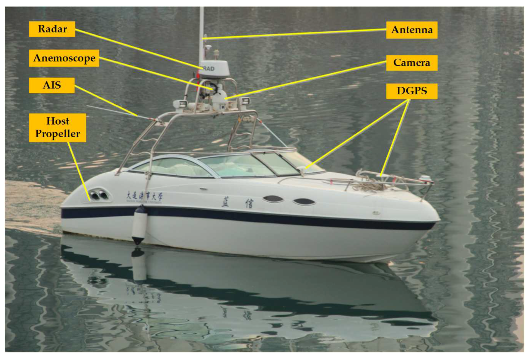
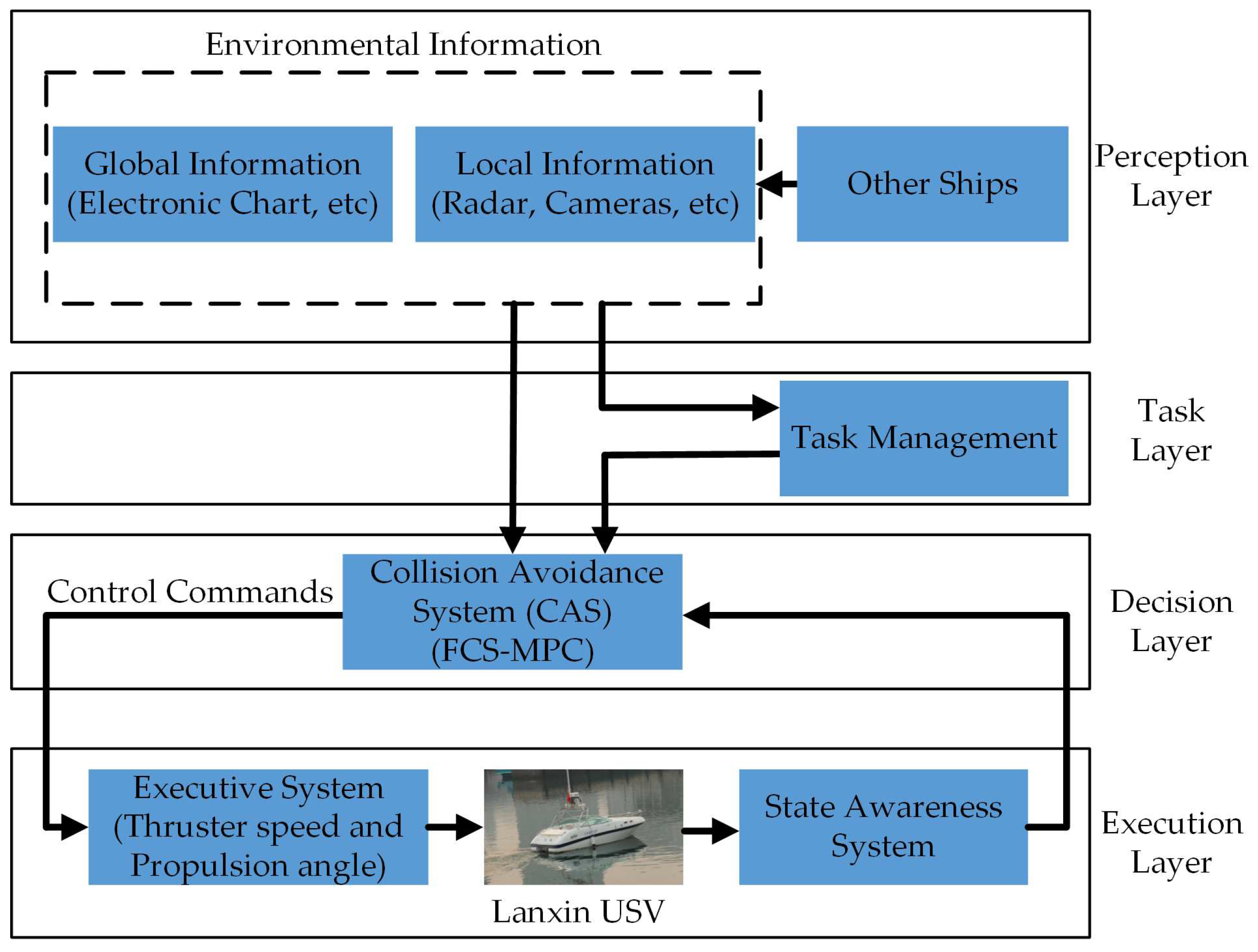
2. The Overview of the System Structure and Technology
3. Collision Avoidance Based on the Finite Control Set Model Predictive Control Method
3.1. Mathematical Model of USV Plane Motion
- The sea environment is calm, so the disturbances caused by environmental factors such as wind, wave and current are neglected;
- The USV is symmetrical, and its barycenter coincides with the geometric center, that is the inertia, added mass and damping matrices are diagonal.
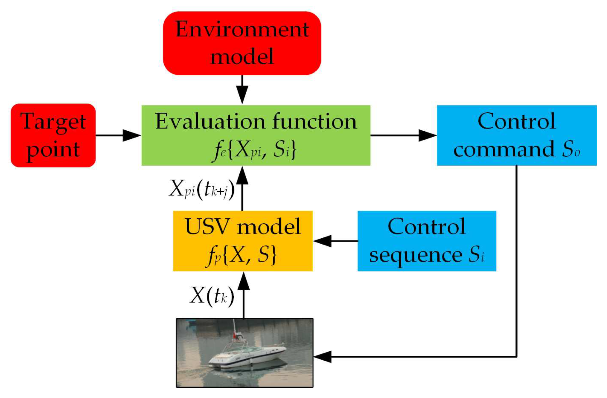
3.2. Finite Control Set Model Predictive Control of CAS
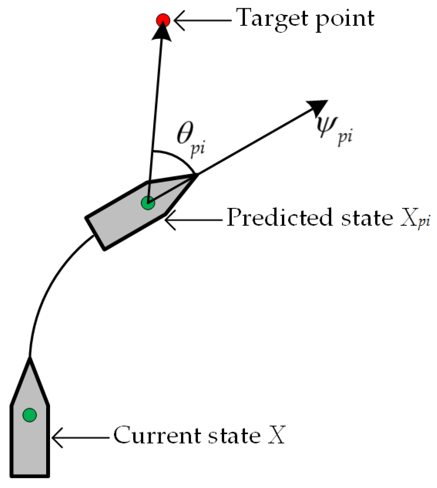
3.3. Control Behaviors and Prediction of USV Trajectory
3.4. Evaluation Function
4. Simulation Study and Results
4.1. Collision Avoidance in a Complex Environment
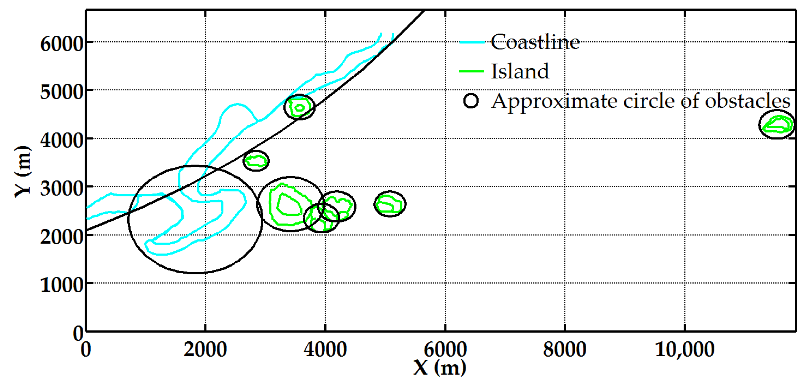
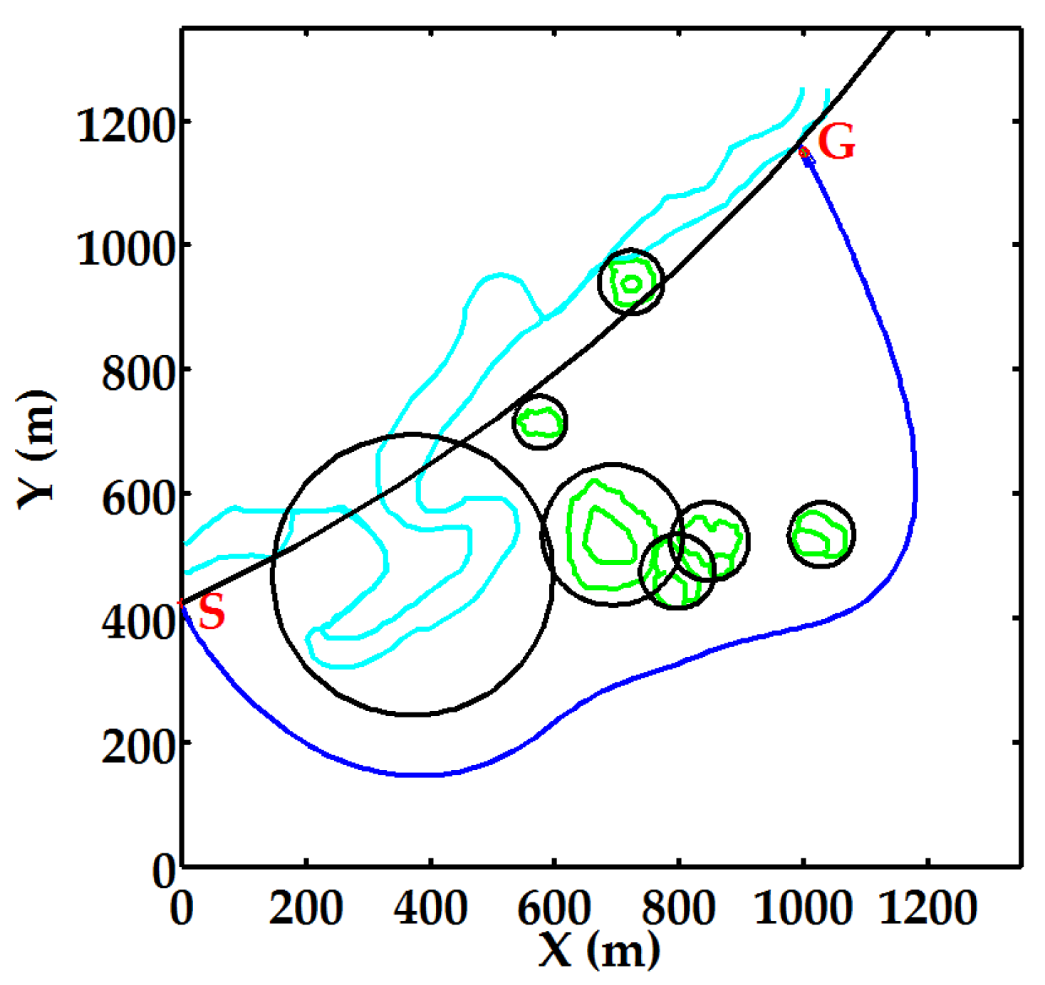
4.2. Collision Avoidance in a Real Environment
4.2.1. Environmental Assumptions
4.2.2. Actual Marine Environment Model
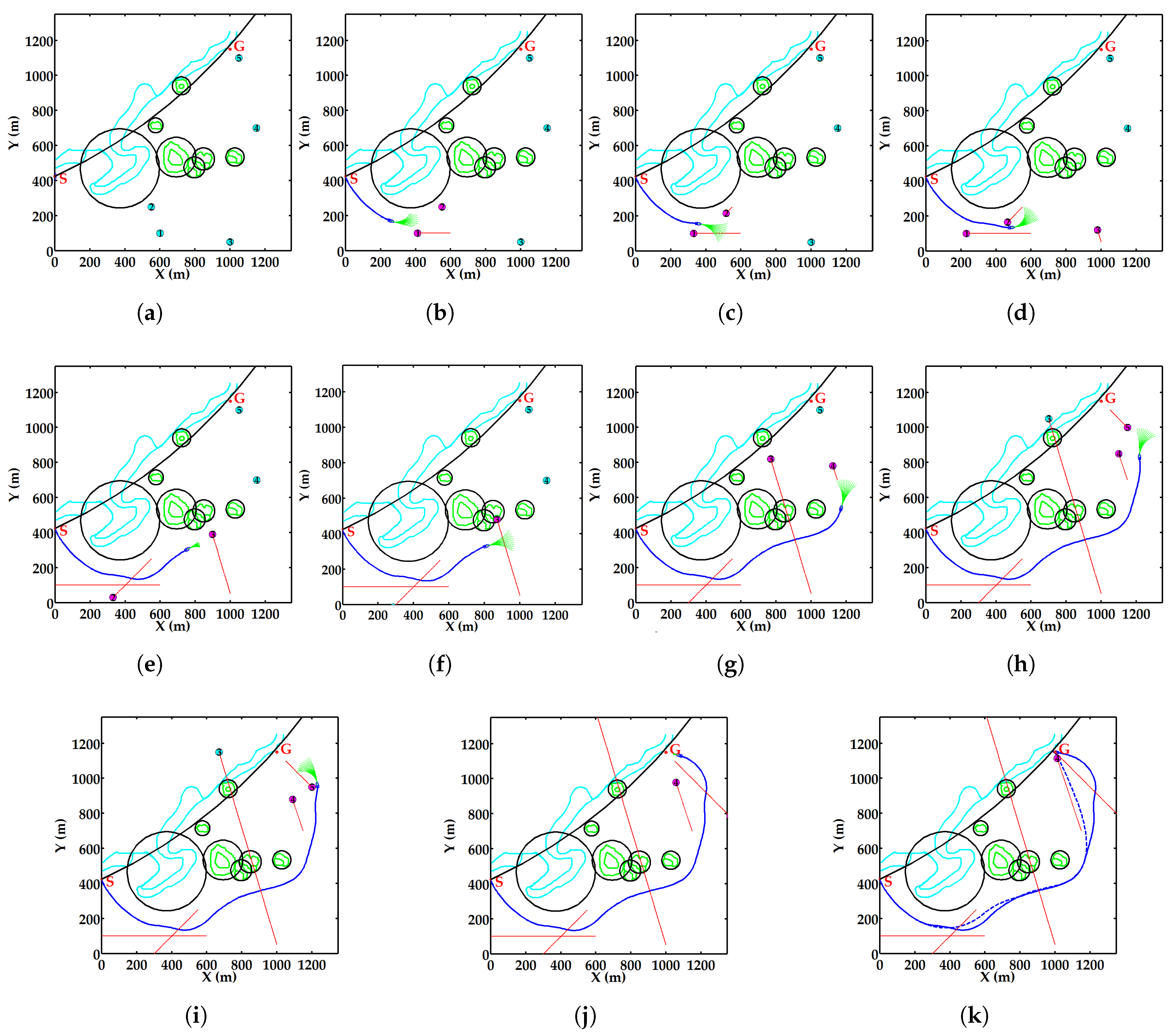
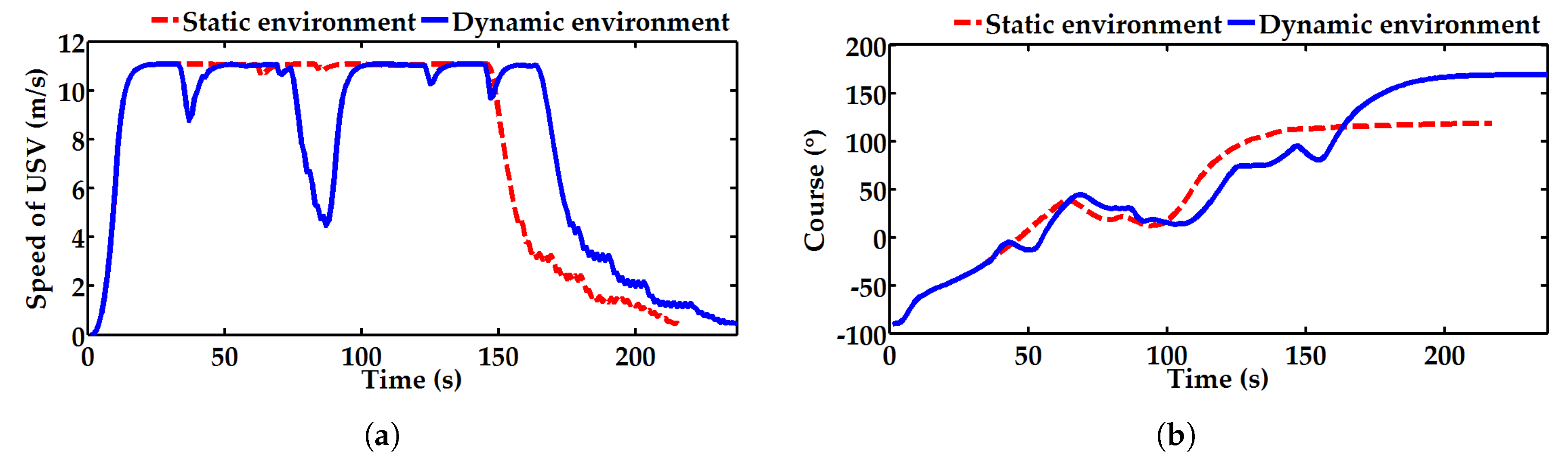
4.2.3. Simulation Verification
5. Conclusions
Author Contributions
Funding
Conflicts of Interest
References
- Campbell, S.; Naeem, W.; Irwin, G.W. A review on improving the autonomy of unmanned surface vehicles through intelligent collision avoidance manoeuvres. Annu. Rev. Control 2012, 36, 267–283. [Google Scholar] [CrossRef]
- Liu, Z.; Zhang, Y.; Yu, X.; Yuan, C. Unmanned surface vehicles: An overview of developments and challenges. Annu. Rev. Control 2016, 41, 71–93. [Google Scholar] [CrossRef]
- Yang, J.M.; Tseng, C.M.; Tseng, P.S. Path planning on satellite images for unmanned surface vehicles. Int. J. Naval Archit. Ocean Eng. 2015, 7, 87–99. [Google Scholar] [CrossRef]
- Kim, H.; Kim, D.; Shin, J.U.; Kim, H.; Myung, H. Angular rate-constrained path planning algorithm for unmanned surface vehicles. Ocean Eng. 2014, 84, 37–44. [Google Scholar] [CrossRef]
- Xie, S.; Wu, P.; Liu, H.; Yan, P.; Li, X.; Luo, J.; Li, Q. A novel method of unmanned surface vehicle autonomous cruise. Ind. Robot 2016, 43, 121–130. [Google Scholar] [CrossRef]
- Wu, P.; Xie, S.; Liu, H.; Li, M.; Li, H.; Peng, Y.; Li, X.; Luo, J. Autonomous obstacle avoidance of an unmanned surface vehicle based on cooperative manoeuvring. Ind. Robot 2017, 44, 64–74. [Google Scholar] [CrossRef]
- Candeloro, M.; Lekkas, A.M.; Sørensen, A.J. A Voronoi-diagram-based dynamic path-planning system for underactuated marine vessels. Control Eng. Pract. 2017, 61, 41–54. [Google Scholar] [CrossRef]
- Campbell, S.; Abu-Tair, M.; Naeem, W. An automatic COLREGs-compliant obstacle avoidance system for an unmanned surface vehicle. Proc. Inst. Mech. Eng. Part M J. Eng. Marit. Environ. 2014, 228, 108–121. [Google Scholar] [CrossRef]
- Kuwata, Y.; Wolf, M.T.; Zarzhitsky, D.; Huntsberger, T.L. Safe Maritime Autonomous Navigation With COLREGS, Using Velocity Obstacles. IEEE J. Ocean. Eng. 2014, 39, 110–119. [Google Scholar] [CrossRef]
- Tang, P.; Zhang, R.; Liu, D.; Huang, L.; Liu, G.; Deng, T. Local reactive obstacle avoidance approach for high-speed unmanned surface vehicle. Ocean Eng. 2015, 106, 128–140. [Google Scholar] [CrossRef]
- Fukushima, H.; Kon, K.; Matsuno, F. Model Predictive Formation Control Using Branch-and-Bound Compatible With Collision Avoidance Problems. IEEE Trans. Robot. 2013, 29, 1308–1317. [Google Scholar] [CrossRef]
- Ji, J.; Khajepour, A.; Melek, W.W.; Huang, Y. Path Planning and Tracking for Vehicle Collision Avoidance Based on Model Predictive Control With Multiconstraints. IEEE Trans. Veh. Technol. 2017, 66, 952–964. [Google Scholar] [CrossRef]
- Mayne, D.Q.; Raković, S. Model predictive control of constrained piecewise affine discrete-time systems. Int. J. Robust Nonlinear Control 2003, 13, 261–279. [Google Scholar] [CrossRef]
- Richards, A.; How, J.P. Robust distributed model predictive control. Int. J. Control 2007, 80, 1517–1531. [Google Scholar] [CrossRef]
- Michael, H.; Matveev, A.S.; Savkin, A.V. Algorithms for collision-free navigation of mobile robots in complex cluttered environments: A survey. Robotica 2015, 33, 463–497. [Google Scholar]
- Scokaert, P.O.M.; Mayne, D.Q. Min-max feedback model predictive control for constrained linear systems. IEEE Trans. Autom. Control 1998, 43, 1136–1142. [Google Scholar] [CrossRef]
- Ntousakis, I.A.; Nikolos, L.K.; Papageorgiou, M. Optimal vehicle trajectory planning in the context of cooperative merging on highways. Transp. Res. Part C Emerg. Technol. 2016, 71, 464–488. [Google Scholar] [CrossRef]
- Johansen, T.A.; Perez, T.; Cristofaro, A. Ship Collision Avoidance and COLREGS Compliance Using Simulation-Based Control Behavior Selection With Predictive Hazard Assessment. IEEE Trans. Intell. Transp. Syst. 2016, 17, 3407–3422. [Google Scholar] [CrossRef]
- Formentini, A.; Trentin, A.; Marchesoni, M.; Zanchetta, P.; Wheeler, P. Speed Finite Control Set Model Predictive Control of a PMSM Fed by Matrix Converter. IEEE Trans. Ind. Electron. 2015, 62, 6786–6796. [Google Scholar] [CrossRef]
- Mu, D.D.; Wang, G.F.; Fan, Y.S. Design of Adaptive Neural Tracking Controller for Pod Propulsion Unmanned Vessel Subject to Unknown Dynamics. J. Electr. Eng. Technol. 2017, 12, 2365–2377. [Google Scholar]
- Zhang, R.; Li, K.; He, Z.; Wang, H.; You, F. Advanced Emergency Braking Control Based on a Nonlinear Model Predictive Algorithm for Intelligent Vehicles. Appl. Sci. 2017, 7, 504. [Google Scholar] [CrossRef]
- Chen, S.L.; Cheng, C.Y.; Hu, J.S.; Jiang, J.F.; Chang, T.K.; Wei, H.Y. Strategy and Evaluation of Vehicle Collision Avoidance Control via Hardware-in-the-Loop Platform. Appl. Sci. 2016, 6, 327. [Google Scholar] [CrossRef]
- Yao, P.; Wang, H.L.; Su, Z.K. Real-time path planning of unmanned aerial vehicle for target tracking and obstacle avoidance in complex dynamic environment. Aerosp. Sci. Technol. 2015, 47, 269–279. [Google Scholar] [CrossRef]
- Zuhaib, K.M.; Khan, A.M.; Iqbal, J.; Ali, M.A.; Usman, M.; Ali, A.; Yaqub, S.; Lee, J.Y.; Han, C. Collision Avoidance from Multiple Passive Agents with Partially Predictable Behavior. Appl. Sci. 2017, 7, 903. [Google Scholar] [CrossRef]
- Fossen, T.I. Marine Control Systems: Guidance, Navigation and Control of Ships, Rigs and Underwater Vehicles; Marine Cybernetics: Trondheim, Norway, 2002. [Google Scholar]
- Mu, D.; Wang, G.; Fan, Y.; Sun, X.; Qiu, B. Adaptive LOS Path Following for a Podded Propulsion Unmanned Surface Vehicle with Uncertainty of Model and Actuator Saturation. Appl. Sci. 2017, 7, 1232. [Google Scholar] [CrossRef]
- Dong, W.; Guo, Y. Global time-varying stabilization of underactuated surface vessel. IEEE Trans. Autom. Control 2005, 50, 859–864. [Google Scholar] [CrossRef]
- Fossen, T.I. Guidance and Control of Ocean Vehicles; John Wiley & Sons Inc.: Hoboken, NJ, USA, 1994. [Google Scholar]
- Jia, X.L.; Yang, Y.S. The Mathematical Model of Ship Motion Mechanism Modeling and Identification Modeling; Dalian Maritime University Press: Dalian, China, 1999. [Google Scholar]
- Sun, X.J.; Shi, L.L.; Fan, Y.S.; Wang, G.F. Online Parameter Identiflcation of USV Motion Model. Navig. China 2016, 1, 39–43. [Google Scholar]
- Wang, N.; Meng, X.; Xu, Q.; Wang, Z. A unified analytical framework for ship domains. J. Navig. 2009, 62, 643–655. [Google Scholar] [CrossRef]


| Parameter | Value | Units | |
|---|---|---|---|
| USV | Initial speed of USV | 0.0 (0.0) | m/s (kn) |
| Initial thruster speed | 0.0 | r/min | |
| Maximum thruster speed | 66.7 (4000) | r/s (r/min) | |
| Change rate of thruster speed | 6.7 | r/s2 | |
| Discrete thruster speed | 1.7 (100) | r/s (r/min) | |
| Initial propulsion angle | 0.0 | ||
| Maximum propulsion angle | 30.0 | ||
| Change rate of propulsion angle | 5.0 | /s | |
| Discrete propulsion angle | 1.0 | ||
| CAS | Detection area | 250.0 | m |
| Distance range | 200.0 | m | |
| Prediction horizon | 15.0 | s | |
| Control update interval | 1.0 | s | |
| Weight of evaluation function | (0.70, 1.50, 1.50, 0.50) | – |
| Start Point (m) | Start Time (s) | Velocity (m/s) | Speed (kn) | |
|---|---|---|---|---|
| Dynamic Obstacle 1 | (300, 500) | 15 | (6, −6) | 16.5 |
| Dynamic Obstacle 2 | (600, 700) | 40 | (0, −10) | 19.4 |
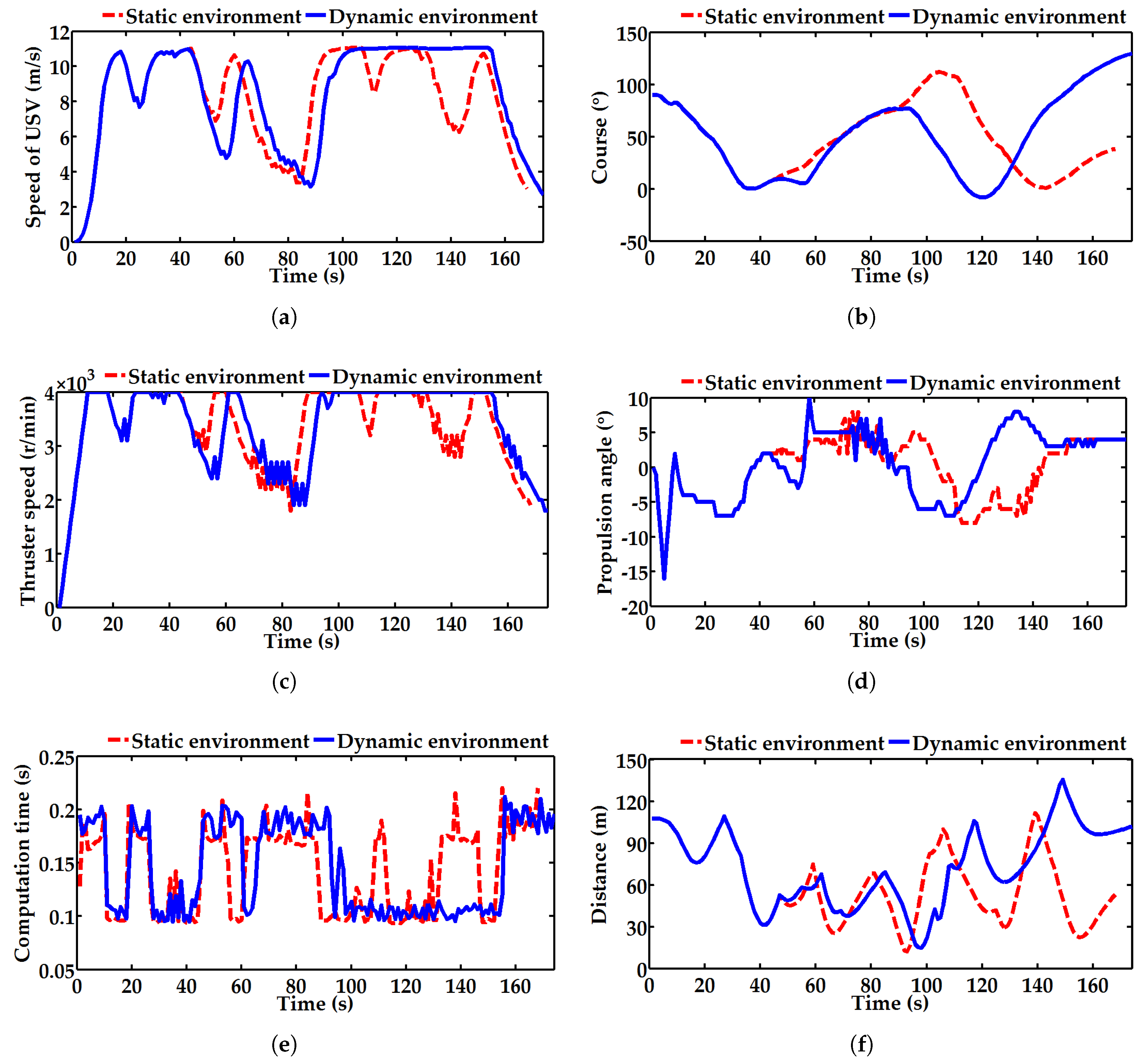
| Environment | Index | Speed of USV (m/s) | Thruster Speed (r/min) | Propulsion Angle () | Computation Time (s) | Distance (m) |
|---|---|---|---|---|---|---|
| static | maximum | 11.1 | 4000 | 8.0 | 0.22 | 111.5 |
| minimum | 0.0 | 0 | −16.0 | 0.09 | 12.2 | |
| average | 8.3 | 3375 | −0.5 | 0.14 | 60.2 | |
| dynamic | maximum | 11.1 | 4000 | 10.0 | 0.21 | 135.5 |
| minimum | 0.0 | 0 | −16.0 | 0.09 | 14.9 | |
| average | 8.4 | 3389 | 0.4 | 0.14 | 72.8 |
| Start Point (m) | Start Time (s) | Velocity (m/s) | Speed (kn) | |
|---|---|---|---|---|
| Dynamic Obstacle 1 | (600, 100) | 20 | (−10, 0) | 19.4 |
| Dynamic Obstacle 2 | (550, 250) | 40 | (−5, −5) | 13.7 |
| Dynamic Obstacle 3 | (1000, 50) | 50 | (−3, −10) | 20.3 |
| Dynamic Obstacle 4 | (1150, 700) | 100 | (−1, 3) | 6.1 |
| Dynamic Obstacle 5 | (1050, 1100) | 130 | (5, −5) | 13.7 |
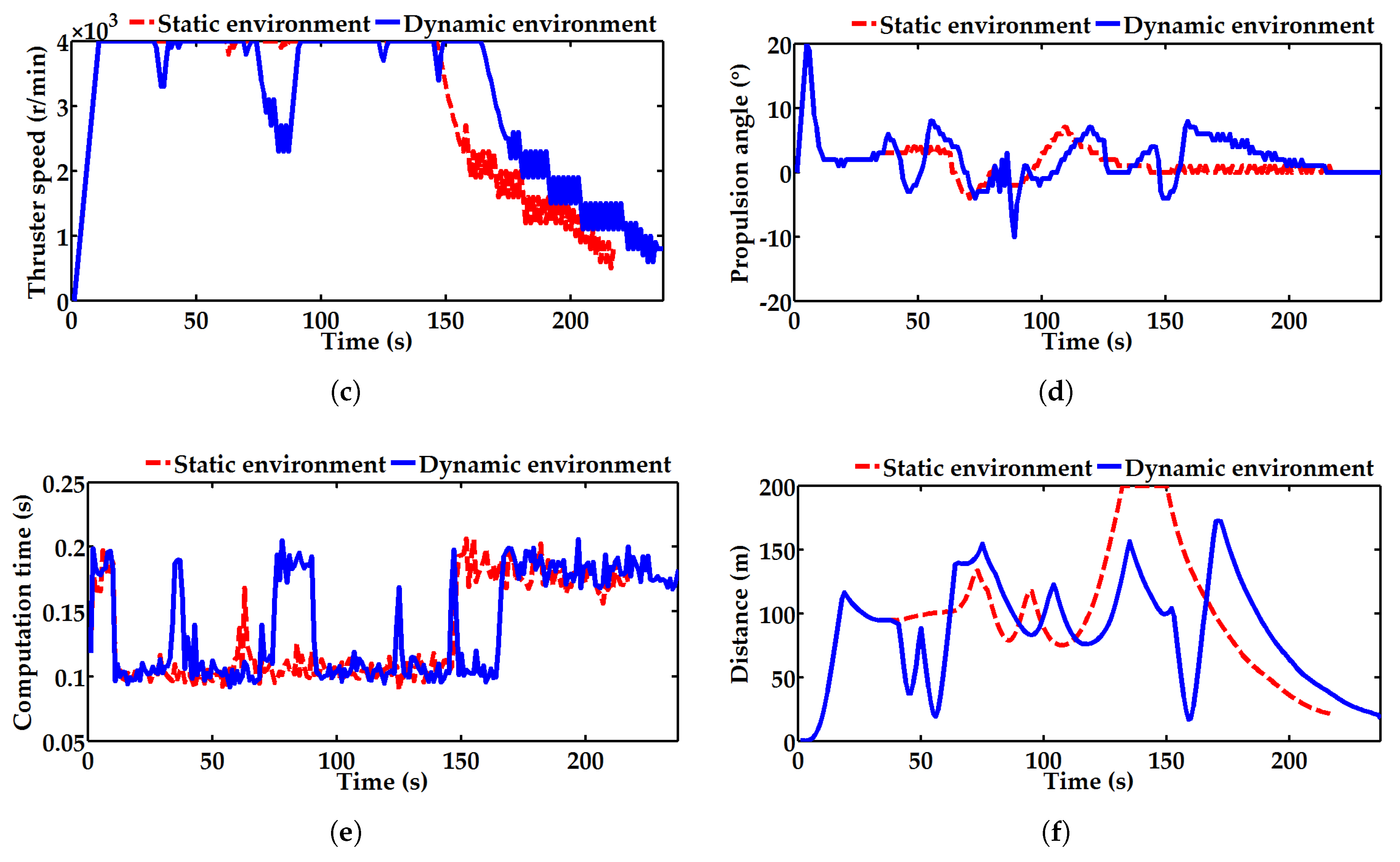
| Environment | Index | Speed of USV (m/s) | Thruster Speed (r/min) | Propulsion Angle () | Computation Time (s) | Distance (m) |
|---|---|---|---|---|---|---|
| static | maximum | 11.1 | 4000 | 20.0 | 0.21 | 200.0 |
| minimum | 0.0 | 0 | −4.0 | 0.09 | 75.1 | |
| average | 7.9 | 3153 | 1.7 | 0.13 | 116.3 | |
| dynamic | maximum | 11.1 | 4000 | 20.0 | 0.21 | 172.4 |
| minimum | 0.0 | 0 | −10.0 | 0.09 | 16.7 | |
| average | 7.7 | 3117 | 2.1 | 0.14 | 97.6 |
© 2018 by the authors. Licensee MDPI, Basel, Switzerland. This article is an open access article distributed under the terms and conditions of the Creative Commons Attribution (CC BY) license (http://creativecommons.org/licenses/by/4.0/).
Share and Cite
Sun, X.; Wang, G.; Fan, Y.; Mu, D.; Qiu, B. Collision Avoidance Using Finite Control Set Model Predictive Control for Unmanned Surface Vehicle. Appl. Sci. 2018, 8, 926. https://doi.org/10.3390/app8060926
Sun X, Wang G, Fan Y, Mu D, Qiu B. Collision Avoidance Using Finite Control Set Model Predictive Control for Unmanned Surface Vehicle. Applied Sciences. 2018; 8(6):926. https://doi.org/10.3390/app8060926
Chicago/Turabian StyleSun, Xiaojie, Guofeng Wang, Yunsheng Fan, Dongdong Mu, and Bingbing Qiu. 2018. "Collision Avoidance Using Finite Control Set Model Predictive Control for Unmanned Surface Vehicle" Applied Sciences 8, no. 6: 926. https://doi.org/10.3390/app8060926
APA StyleSun, X., Wang, G., Fan, Y., Mu, D., & Qiu, B. (2018). Collision Avoidance Using Finite Control Set Model Predictive Control for Unmanned Surface Vehicle. Applied Sciences, 8(6), 926. https://doi.org/10.3390/app8060926