An Intelligent Fault Diagnosis Approach Considering the Elimination of the Weight Matrix Multi-Correlation

Abstract

Faults in bearings and gearboxes, which are widely used in rotating machines, can lead to heavy investment and productivity loss. Accordingly, a fault diagnosis system is necessary to ensure a high-performance transmission. However, as mechanical fault diagnosis enters the era of big data, it can be difficult to apply traditional fault diagnosis methods because of the massive computation cost and excessive reliance on human labor. Meanwhile, unsupervised learning has been shown to have excellent performance in processing machanical big data. In this paper, an unsupervised learning method known as sparse filtering is applied, the multi-correlation of a weight matrix is investigated, and a method that is more suitable for the feature extraction of signals is proposed. The main contribution of our work is the modification of original method. First, to understand the non-monotonicity testing accuracies of the original method, the physical interpretation of input dimensions is studied. Second, using the physical interpretation, an overfitting phenomenon is discovered and examined. Third, to reduce the overfitting phenomenon, a method which eliminates the multi-correlation of the weight matrix is proposed. Finally, bearing and gear datasets are employed to verify the effectiveness of the proposed method; experimental results show that the proposed method can achieve a superior performance in comparison to the original sparse filtering model.

1. Introduction

With the arrival of modern manufacturing systems, machines have become more automatic and efficient, which has led to increased demands on their reliability, quality, and availability [1,2]. As a result, machinery fault diagnosis systems, which focus on the detection of health conditions after the occurrence of certain faults, have attracted considerable attention [3,4]. Additionally, with recent developments in both industry and the Internet, data acquisition has exponentially increased. Thus, fault diagnosis has entered the era of Big Data [5,6,7]. Because mechanical big data is typically characterized as large-volume, diverse, and of high-velocity [8], methods of extracting features rapidly and accurately from mechanical big data has become an urgent subject of research [9,10]. Existing fault diagnosis methods can be divided into two major categories [11]: physics-based models and data-driven ones [12,13]. Physics-based models overly rely on high-quality domain knowledge and necessitate massive computation costs, which reduces the overall efficiency of fault diagnosis. Thus, it is unsuitable for big data [14,15,16]. The data-driven models [15], such as Artificial Neural Networks (ANN) [17,18], Autoencoders [5], Restricted Boltzmann Machine (RBM) [19], Convolutional Neural Networks (CNN) [20,21], and k-Nearest Neighbor [22], depend less on human knowledge and can effectively diagnose faults in mechanical big data. However, these intelligent fault diagnosis methods pose specific challenges, e.g., a difficulty in adjusting various hyperparameters, and good diagnosis accuracy can be obtained only when the hyperparameters are set properly. For example, Autoencoder has four hyperparameters to tune while RBM has six.

Ngiam [23] proposed a sparse filtering method: an unsupervised two-layer network which optimizes the sparsity distribution of the features calculated by the collected data instead of modeling the distribution of the data. It also scales well with the dimension of the input [24]. Only the number of features needs to set; as a result, it is extremely simple to tune and easy to implement. Thanks to this strong performance, sparse filtering has been successfully adopted in several image recognition cases [25,26,27]. Recently, sparse filtering also has been introduced into the field of rotary machinery fault diagnosis, delivering excellent performance in feature extraction from complex fault signals. As is well known, Lei et al. [28] first made a constructive attempt to apply sparse filtering to fault diagnosis by a two-stage learning method. As a result, sparse filtering was proved to be an excellent tool for feature extraction. Subsequently, a physical interpretation to sparse filtering was achieved, in which trained weight vectors could be compared directly to the Gabor filters. Zhao et al. [29] used sparse filtering to extract multi-domain sparse features and adopted it for fault identification in a planetary gearbox. Jiang et al. [30] proposed a multiscale representation learning (MSRL) framework, which was based on sparse filtering, to learn useful features from a direct interpretation of raw vibration signals; the aim was to capture rich and complementary fault pattern information at different scales. Yang et al. [31] combined sparse filtering with a Support Vector Machine optimized by a Improved Particle Swarm to simplify the hyperparameters.

However, as shown in Lei et al. [28], when the important parameter of input dimension increased, an initial increase in testing accuracies was followed by a marked decrease (in this paper, the rule is called non-monotonicity). This indicates considerable time is required to optimize the input dimension to increase diagnosis accuracy. To avoid this unnecessary work, the motivation behind non-monotonicity should be clearly explained. Therefore, the interpretation of input dimensions should be studied first. Next, the nature of non-monotonicity will be explained and, finally, a method to improve the performance of sparse filtering for fault diagnosis will be proposed.

To solve these problems, this paper is organized as follows. Section 2 introduces the algorithm of sparse filtering. Section 3 studies the interpretation of input dimension and explains the nature of the non-monotonicity phenomenon. Section 4 details the proposed method, which is based on the elimination of the multi-correlation of weight matrix. In Section 5, the diagnosis cases of bearing and gear datasets are adopted to validate the effectiveness of the proposed method. Finally, conclusions are drawn in Section 6.

2. Sparse Filtering

Sparse filtering is an unsupervised feature learning method that attempts to ensure learning features satisfy three principles: population sparsity, lifetime sparsity, and high dispersal [23]. To realize these properties, sparse filtering trains a weight matrix through the optimization of a cost function.

As shown in Figure 1, the collected raw vibration signal is used as input data. Firstly, the vibration signal is separated into M samples to compose the training set ${\left\{{\mathit{x}}^i\right\}}_{i=1}^M$, where ${\mathit{x}}^i\in {\Re }^{N\times 1}$ is a training sample which contains N data points. Then, the training set is used to train the sparse filtering model to obtain a weight matrix $\mathit{W}\in {\Re }^{N\times L}$. Finally, each sample is mapped into a feature vector ${\mathit{f}}^i\in {\Re }^{L\times 1}$ by the weight matrix. For sparse filtering, an activation function is needed to calculate the nonlinear features.

We consider the situation that sparse filtering computes linear features for each sample:

$$f_j^i={\mathit{W}}_j^T{\mathit{x}}^i$$

(1)

where $f_j^i$ is the jth feature value.

The feature matrix comprises the features $f_j^i$. Firstly, each row is normalized to be equally activated by its $\ell 2$-norm:

$${\tilde{\mathit{f}}}_j={{\mathit{f}}_j/\Vert {\mathit{f}}_j\Vert }_2$$

(2)

Then, each column (or each sample) is normalized by its $\ell 2$-norm. As a result, each feature is constrained to lie on the unit $\ell 2$-ball:

$${\widehat{\mathit{f}}}^i={{\tilde{\mathit{f}}}^i/\Vert {\tilde{\mathit{f}}}^i\Vert }_2$$

(3)

Finally, the normalized features are optimized for sparseness using the $\ell 1$ penalty. For the training set ${\left\{{\mathit{x}}^i\right\}}_{i=1}^M$, the sparse filtering objective is shown as follows:

$$\mathrm{minimize}\mathrm{J}(\mathit{W})={\displaystyle \sum _{i=1}^M{\Vert {\widehat{\mathit{f}}}^i\Vert }_1}$$

(4)

Generally, the activation function $g(\cdot )=|\cdot |$ is recommended and can be rewritten as the inner product form:

$$f_l^i=g({\mathit{W}}_j^T{\mathit{x}}^i)=\left|{\mathit{W}}_j^T{\mathit{x}}^i\right|=\left|\langle {\mathit{W}}_j^T{\mathit{x}}^i\rangle \right|$$

(5)

This suggests sparse filtering can be interpreted as a measurement of the similarity between the input signals and a series of weight vectors, such as wavelet transform [32].

3. Nature of Input Dimension and Overfitting

In this section, the nature of non-monotonicity is studied. First, several fundamental laws are revealed using a series of harmonic signals. Then, the bearing fault signals are applied to further verify our interpretation. Finally, on the basis of the physical interpretation, the overfitting phenomenon is discovered and the nature of it is investigated.

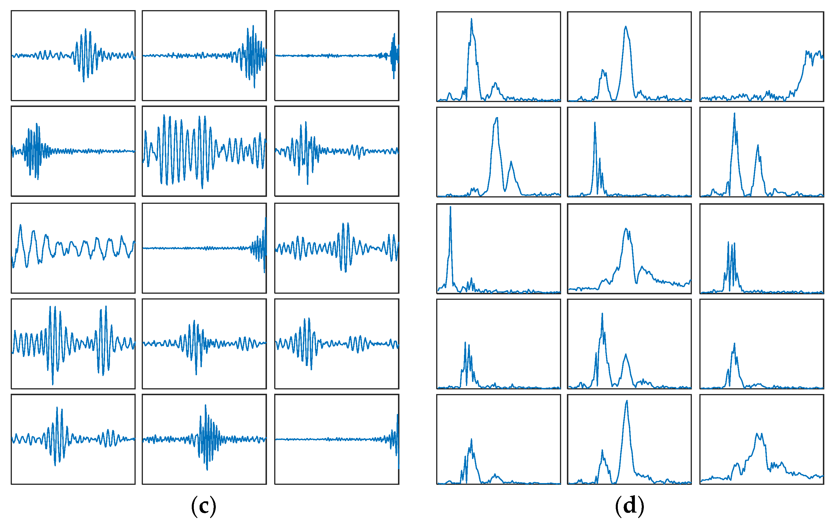
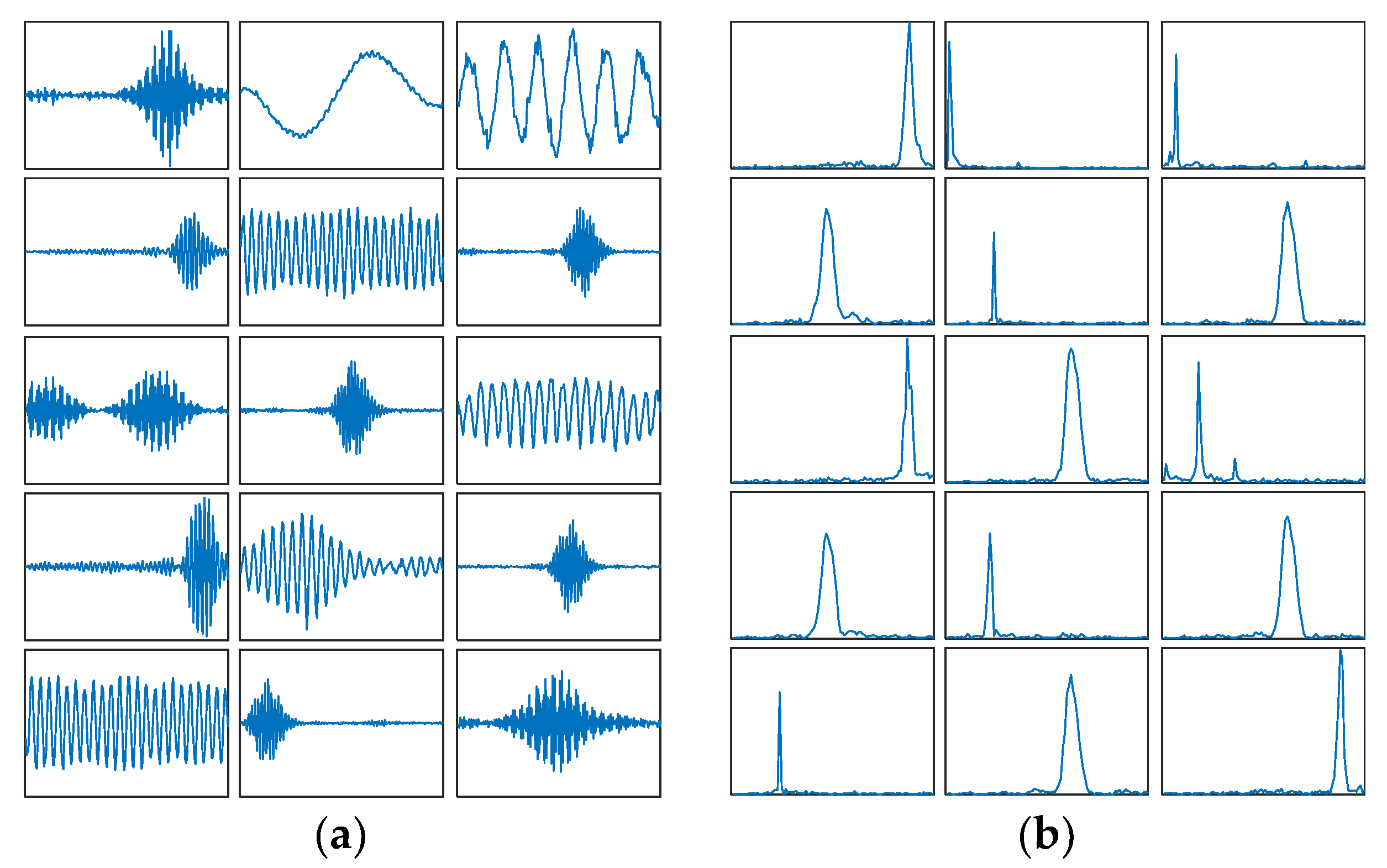
3.1. Characteristics of Harmonic Signals

A harmonic signal y(t) is defined as follows:

$$y(t)=A\sin (2\pi f_{r}t+\theta )$$

(6)

where A and θ are the amplitude and phase of y(t), respectively; f_r denotes the rotational frequency.

The sampling rate f_s of the signals is 10,000 Hz and sampling time t is 12 s. 30 trials were carried out for each experiment in this section to reduce the effect of randomness. In addition, 10% of samples were randomly selected for training and the output dimension was set to 1.

3.1.1. Consider Different Initial Phases

Two harmonic signal groups of frequency (100 Hz and 130 Hz) with different initial phases are exploited through sparse filtering, where A = 1; θ = 0°, 45°, 90°, 135°, 180°, 225°, 270°. The classification results of different input dimensions are displayed in Figure 2. It was determined that, when the input dimension N_in = 50, 100, 150, 200; f_r = 100 Hz, the testing accuracies reached 100%. However, the majority of the testing accuracies were quite low. It is possible that sparse filtering was unable to recognize the information of the initial phase.

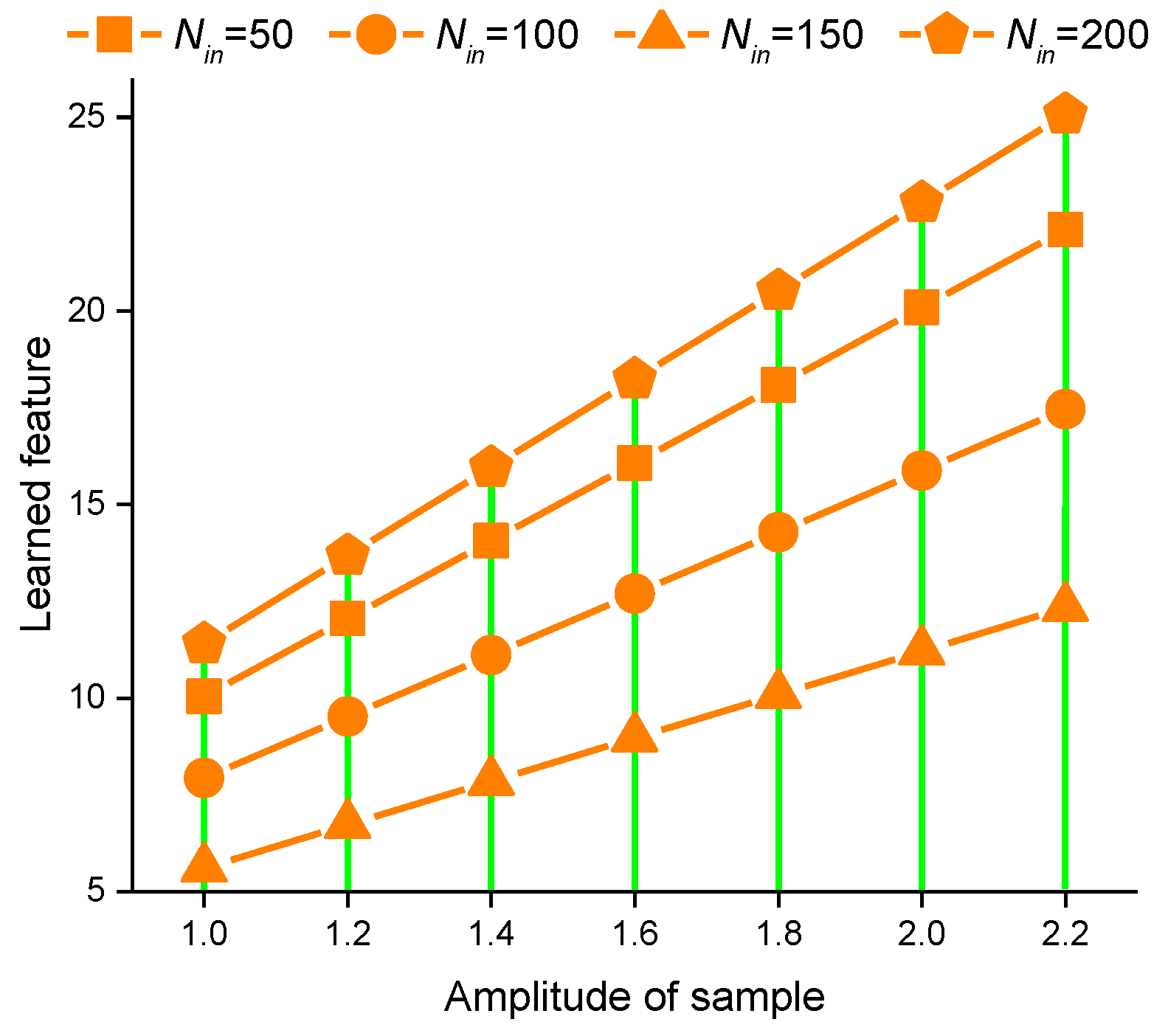
3.1.2. Consider Different Amplitudes

A batch of harmonic signals with different amplitudes were processed based on sparse filtering without loss of generality, where A = 1, 1.2, 1.4, 1.6, 1.8, 2, 2.2; θ = 0°; f_r = 100 Hz. 100% accuracies were obtained with different input dimensions. Figure 3, shows the relationship between the amplitudes of samples and the learned features with different input dimensions. It indicates that the learned features are proportional to the amplitudes of samples. The scales are irregular and do not depend on input dimension. It means that sparse filtering could classify different types by the amplitude information; however, the input dimension does not affect the learned features of sparse filtering. Thus, the amplitude was set at one in the follow-up study.

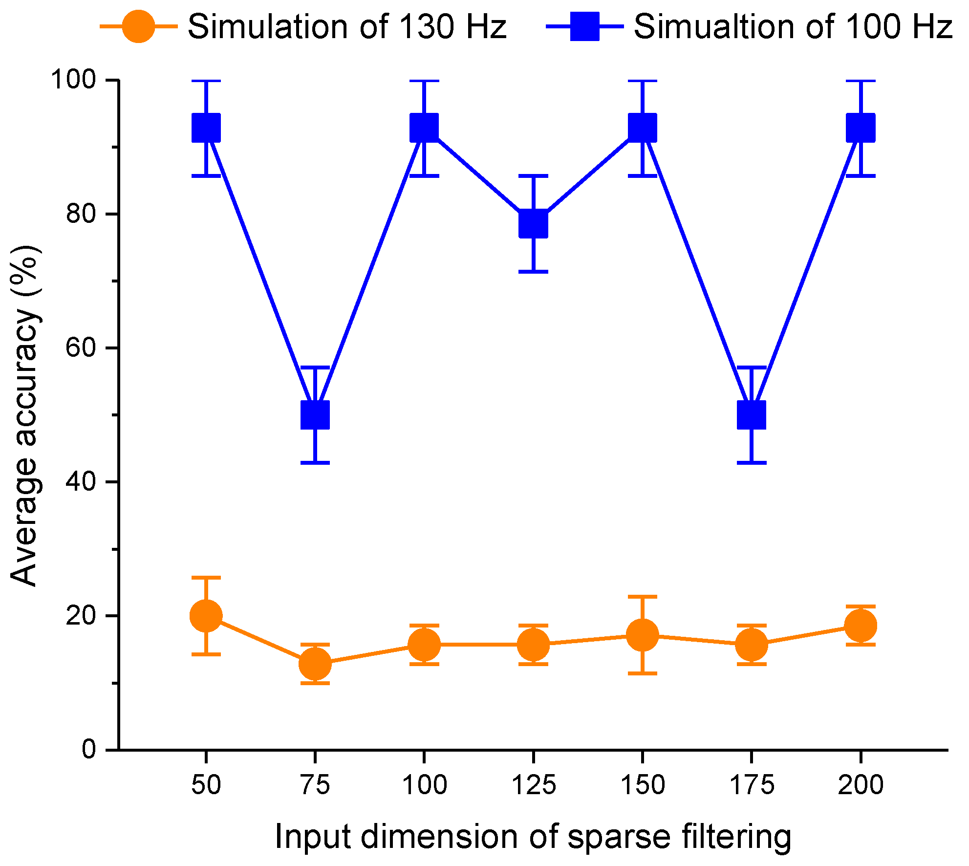
3.1.3. Consider Different Rotational Frequencies

A set of rotational speeds were used to describe the frequency distinguishing ability of sparse filtering, where A = 1; θ = 0°; f_r = 100, 150, 200, 250, 300, 350, 400 Hz. Figure 4 shows the diagnosis accuracies using various input dimensions. The testing accuracy of all input dimensions achieved 100%. This suggests that the learned features of sparse filtering could reflect the frequency information of vibration signals. However, when the input dimension increased, the averaged testing accuracy was higher.

To illustrate this phenomenon, we selected two different output dimensions of weight matrixes for comparison analysis, i.e., 100 and 200. The learned features and the spectra of weight matrixes are shown in Figure 5. It is seen in Figure 5a that the frequency interval in the spectra of weight matrixes was equal to that in the samples, and the amplitudes of spectra were proportional to the features with the corresponding frequency. This resulted in steady, clear, and different learned features within the various samples. However, the frequency interval of weight matrixes was equal to 100 Hz in Figure 5b, twice the size of the frequency interval of samples. The features of several samples, whose frequencies were 150, 250, 350 Hz, depended on the amplitudes of adjacent frequencies in the spectra of the weight matrix. This also resulted in unclear learned features, as in Figure 5b. Therefore, the frequency resolution of weight matrix depends on the input dimension.

From the inspection of the properties of a series of harmonic signals, several conclusions can be summarized:

(1)

Sparse filtering is unable to classify the initial phase information.

(2)

Sparse filtering can recognize the amplitude information, but the input dimension does not affect the learned features of sparse filtering.

(3)

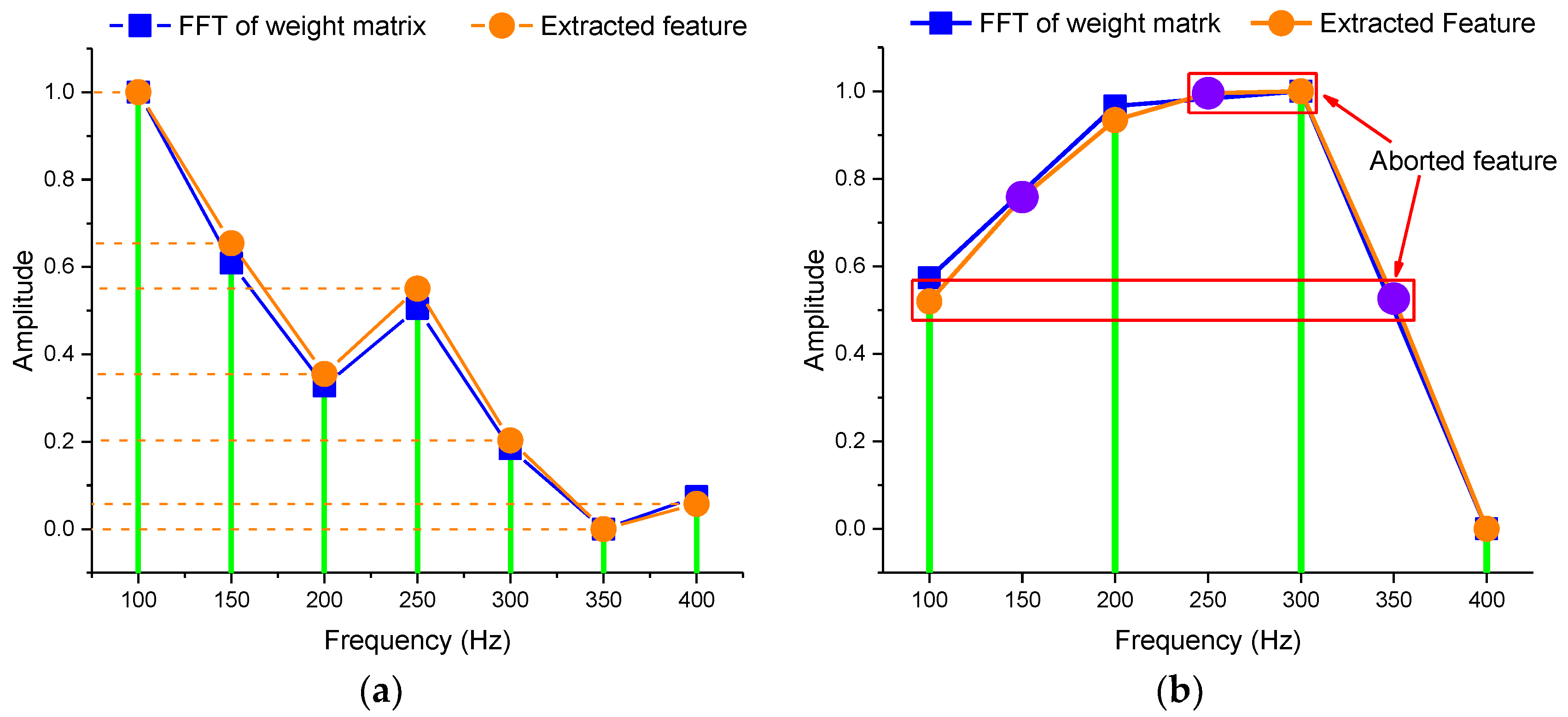
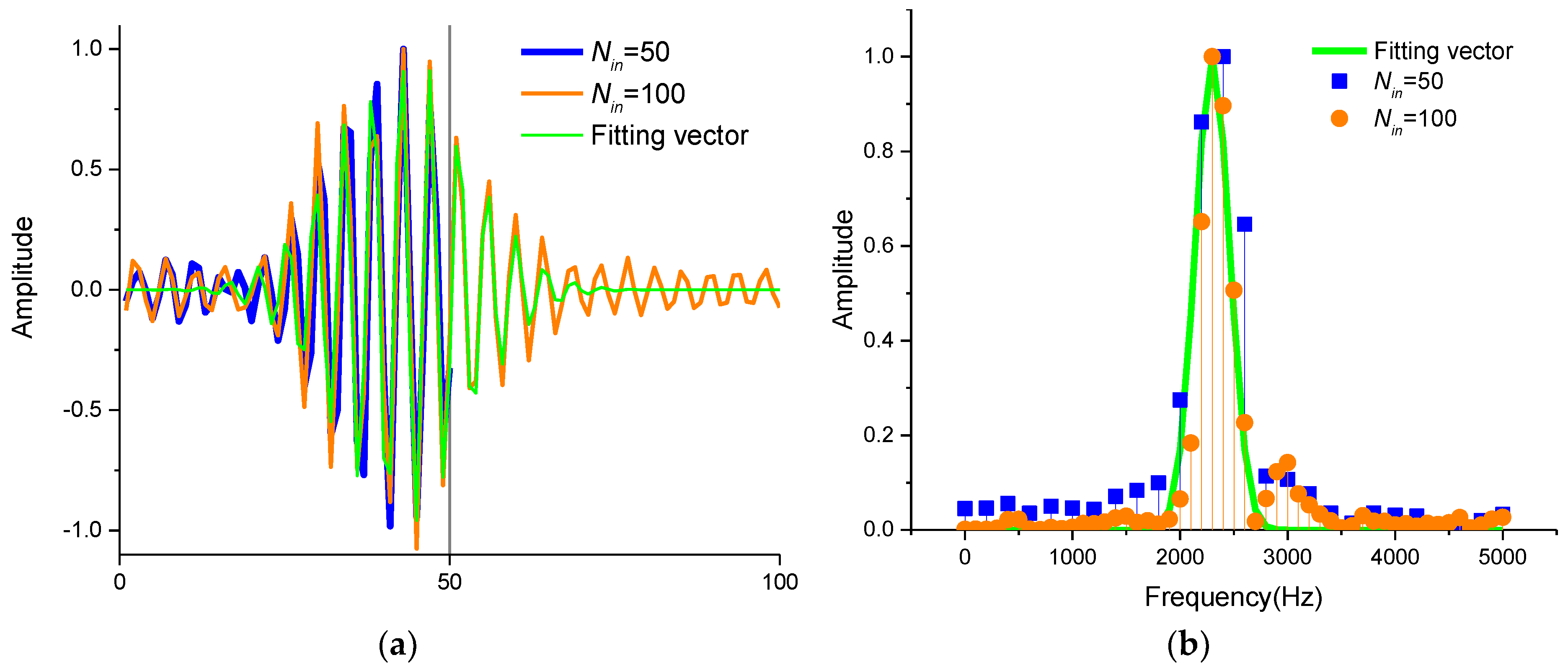
The learned features of sparse filtering can reflect the frequency information. Additionally, the frequency resolution of weight matrix depends on the input dimension. The features are unstable when the input dimension reduces in size.

3.2. Explanation for the Input Dimension Based on Vibration Signals

3.2.1. Data Description

In this section, the bearing dataset [33] provided by Case Western Reserve University were employed for analysis. The vibration signals were collected using accerometers from the drive end of a motor under four different operating conditions: normal condition (NC), inner race fault (IF), outer race fault (OF), and roller fault (RF). There were three different severity levels (0.18, 0.36, and 0.53 mm) for IF, OF, and RF cases, respectively. All the samples were collected under four different loads (0, 1, 2, and 3 hp) and the sampling frequency was 12 kHz. Therefore, the dataset included ten health states under four loads, and we treated the same health state under different loads as one class.

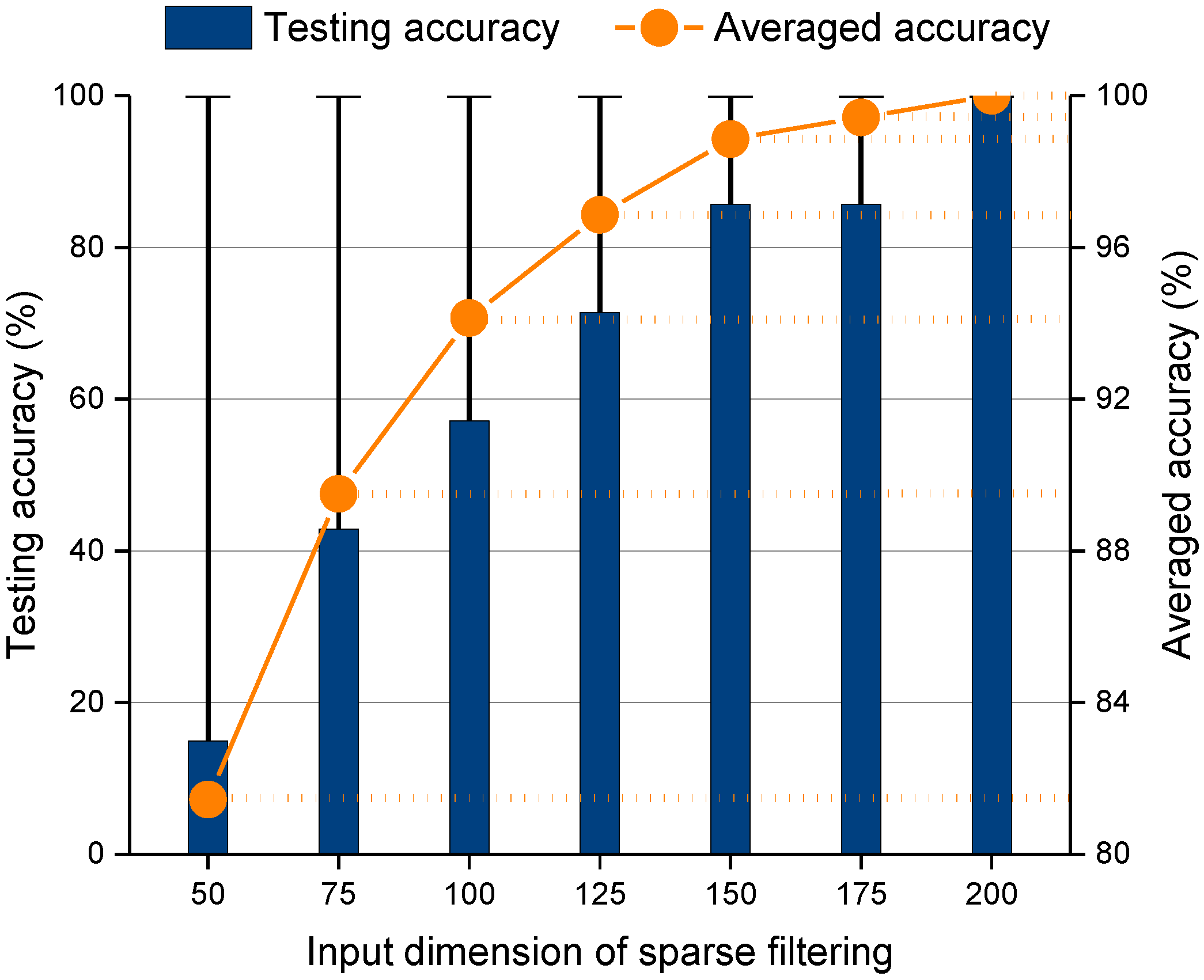
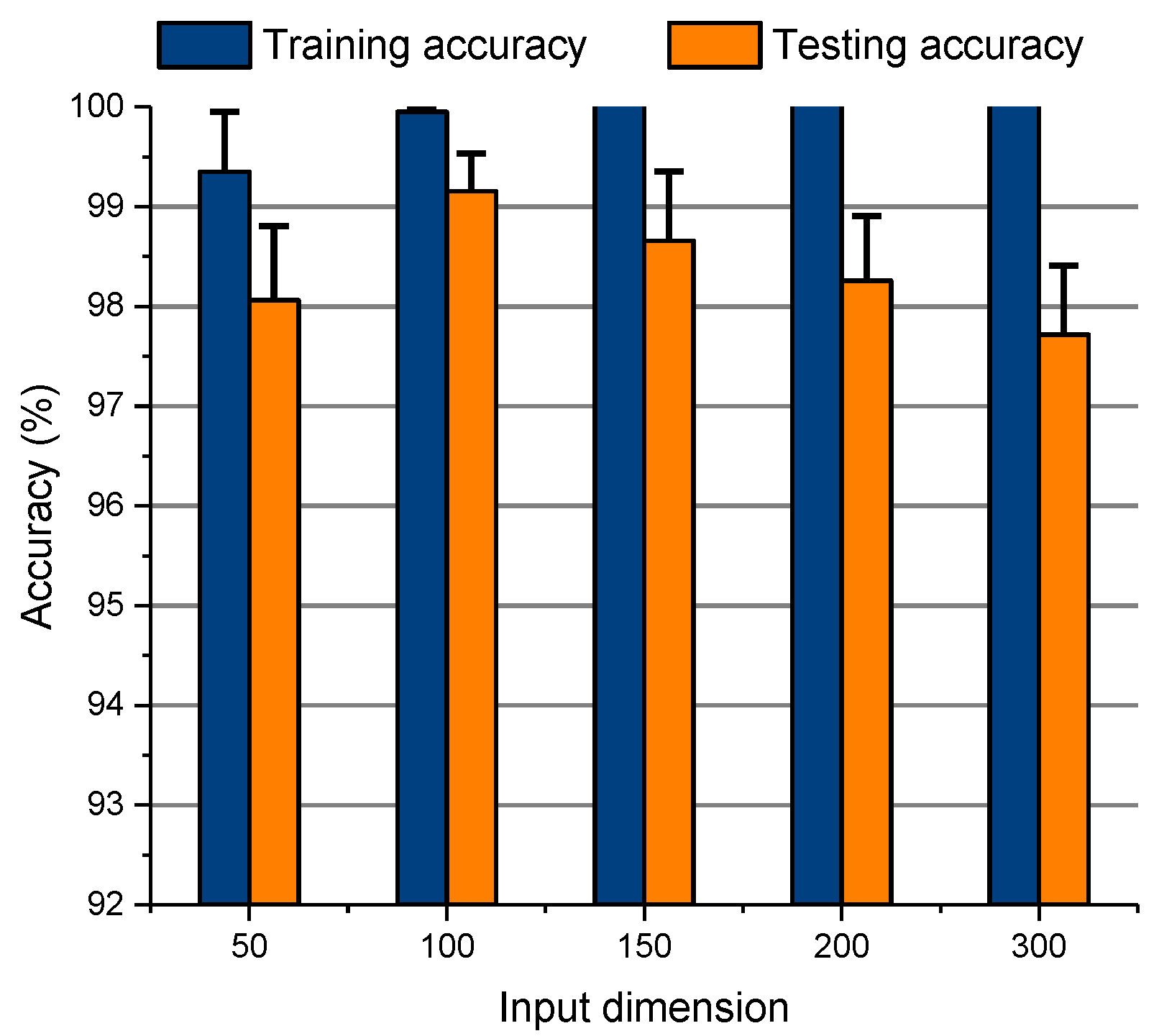
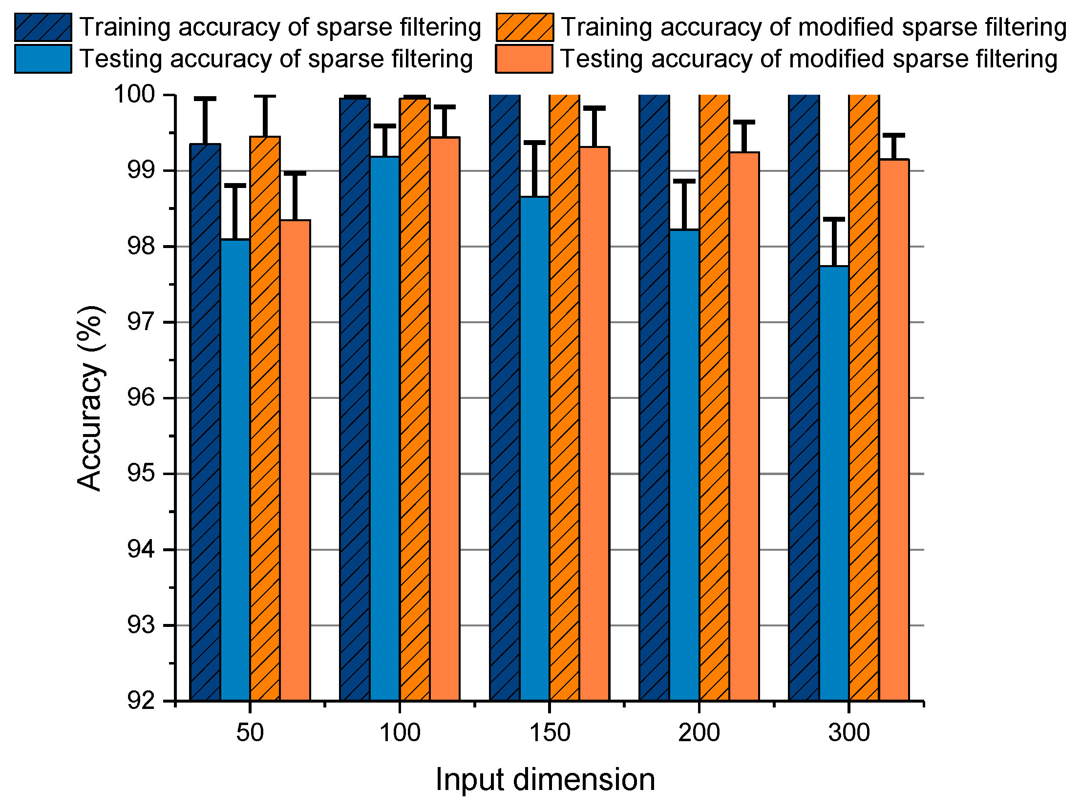
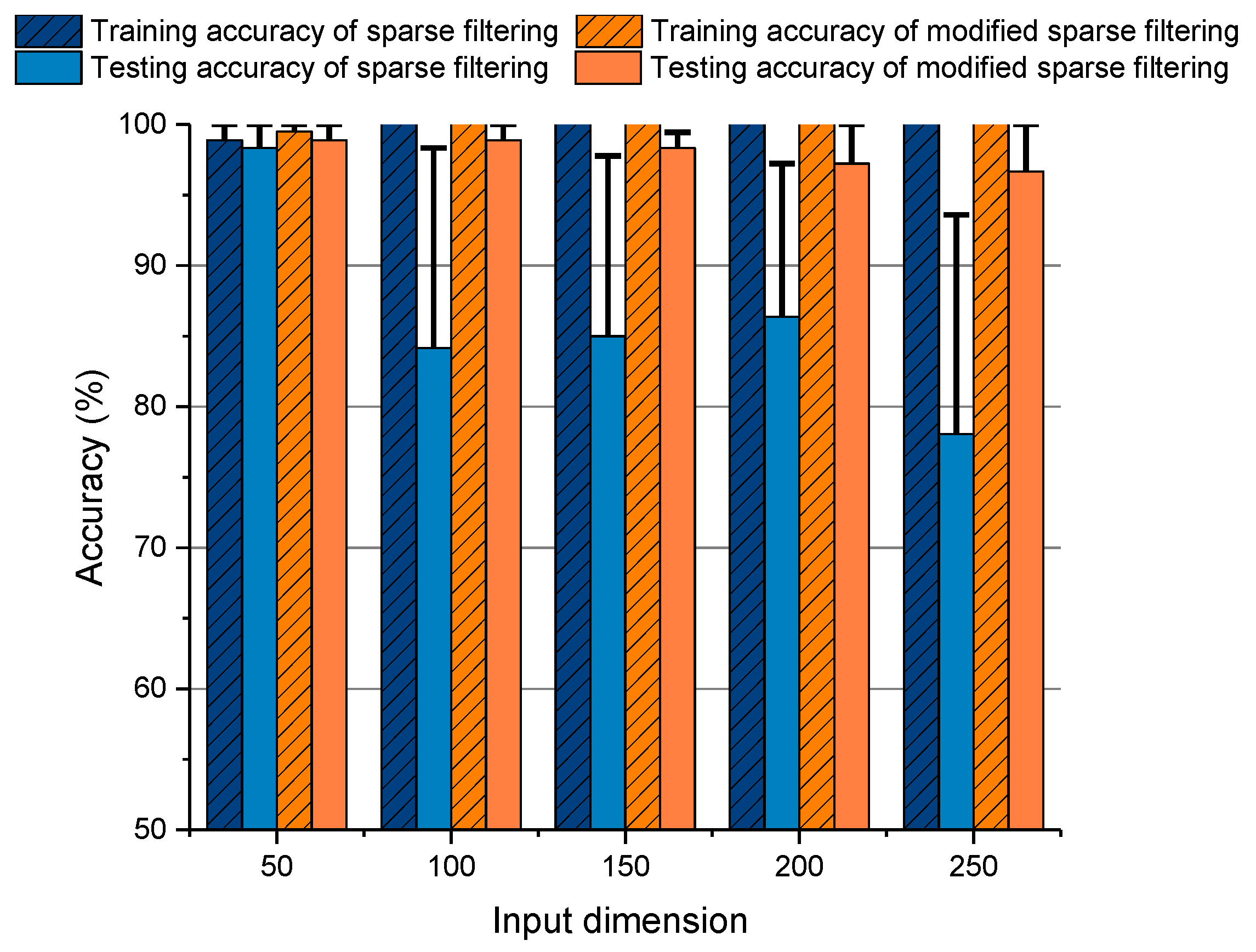
3.2.2. The influence of Input Dimension of Sparse Filtering

The method of Lei et al. [28] was adopted to engage with the experiment signals described above. The selection of input dimension N_in of sparse filtering was investigated. Softmax regression was adopted as a classifier and the diagnosis results are shown in Figure 6. It can be seen that the testing accuracy decreased after an initial increase with the input dimension. Therefore, excessive human labor was required to select the input dimension for the high testing accuracy. To overcome this deficiency, we decided to provide a clear explanation of the nature of the input dimension.

The bearing signals were employed to verify the above explanation of the input dimension on the basis of harmonic signals. As shown in Figure 7a, two weight vectors of N_in = 50 and 100 were selected respectively, and their spectra are shown in Figure 7b. It was determined that the weight vectors were striking similar to the one-dimensional Gabor filter which served as an excellent band-pass filter for signals. The Gabor function is shown as follows [34]:

$$f(d)=A\exp (-\frac{{(d-D)}^2}{2{\sigma }^2})\cos (2\pi \omega (d-D)+\phi )+B$$

(7)

where A, ω, and ϕ are the amplitude, spatial frequency, and phase of the cosine term, respectively, σ is the standard deviation of the Gaussian, D denotes a position offset, and B is an offset parameter. The two different weight vectors exert the same bandwidth, which means that the features extracted by them theoretically have the same frequency information. However, when the input dimension diminishes, the frequency interval of weight matrix also shrinks. As a result, the energy of frequency is dispersed, learning to unclear learned features, which results in lower testing accuracy.

3.3. The Nature of the Overfitting Phenomenon

As seen in the above discussion, the change of input dimension affects testing accuracy through its influence on the frequency resolution of the weight matrix. When the input dimension increased, the testing accuracy also should have increased. However, as seen in Figure 6, when the input dimension was larger than 100, testing accuracy was reduced. Training accuracy did not reduce when the input dimension was increased, suggesting that sparse filtering cannot extract discriminative features for a testing dataset, even though the weight matrix has perfect frequency resolution. This phenomenon is called overfitting.

To explain the nature of overfitting, we use WW^T to measure the similarity of the row vectors respectively when N_in = 100 and N_in = 200. The results can be seen in Figure 8a,b; when the input dimension is 100, the inner product of the same row vector of approaches 1, and the inner product between the two different vectors is close to 0. However, when the input dimension is 200, the inner product of vectors of the weight matrix indicates that they have similar patterns. This suggests that sparse filtering can encourage the learned weight matrix to display clear and distinct patterns when the input dimension is smaller. 15 row vectors of W, trained by sparse filtering with N_in = 100, were randomly selected and plotted in Figure 9a. The corresponding frequency spectra of these row vectors are displayed in Figure 9b. The row vectors show local striking in the time domain and they also dominate the narrow spectral bandwidth in the frequency domain. Accordingly, these row vectors exhibit time-frequency properties and show similarities to one-dimensional Gabor functions, which serve as good band-pass bases for mechanical signals. For comparison, we randomly plotted 15 row vectors of W trained by sparse filtering of N_in = 200 in Figure 9c,d. These vectors also exhibited some time-frequency properties and wide spectral bandwidth in the frequency domain. The results demonstrate that the clearer and more distinct the time-frequency properties of the trained weight matrix are, the better the diagnosis performance of the method. Therefore, sparse filtering encourages learned features to be discriminative to improve the testing accuracy.

4. Modified Sparse Filtering and Two-Stage Learning Method

In this section, a novel method known as modified sparse filtering is proposed, which aims to resolve the problem of overfitting. From the above discussion, the nature of the overfitting phenomenon is that different vectors of the weight matrix exhibit similar patterns. To suppress the similarity of the row vector, a constraint condition is applied to the cost function, which is shown as follows:

$$\mathrm{minimize}\mathrm{J}(\mathit{W})={\displaystyle \sum _{i=1}^M{\Vert {\widehat{\mathit{f}}}^i\Vert }_1}+\lambda {\displaystyle \sum _{i\ne j}\left|{\mathit{\omega }}_i{\mathit{\omega }}_j^T\right|}$$

(8)

where λ is the tuning parameter, ω_iω_j are the vectors of the weight matrix. The constraint condition represents the sum of the inner product among different row vectors.

A two-stage learning method is proposed for intelligent fault diagnosis of machines based on the modified sparse filtering. The illustration and flowchart of the method are shown in Figure 10. In the first learning stage, modified sparse filtering is used to extract local discriminative features from raw vibration signals and the learned features of the signals are obtained by averaging these local features. In the second stage, softmax regression is applied to classify mechanical health conditions using the learned features.

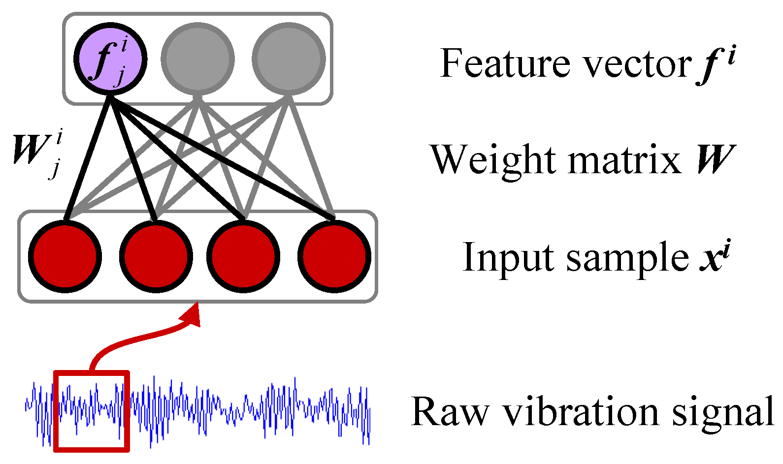
• Collect signals. The vibration signals of machines are obtained under different health conditions. These signals compose the training set ${\{{\mathit{x}}^i,{\mathit{y}}^i\}}_{i=1}^M$, where ${\mathit{x}}^i\in {\Re }^{N\times 1}$ is the ith sample containing M vibration data points and yⁱ is the health condition label. We collect N_s segments from each sample to compose the training set ${\left\{{\mathit{s}}^j\right\}}_{j=1}^{N_s}$ by an overlapped manner, where ${\mathit{s}}^j\in {\Re }^{N_{in}\times 1}$ is the jth segment containing N_in data points. The set ${\left\{{\mathit{s}}^j\right\}}_{j=1}^{N_s}$ is rewritten as a matrix form ${\mathit{S}}^j\in {\Re }^{N_{in}\times N_s}$.
• Whitening. It is necessary to pre-process S by whitening. Whitening uses the eigenvalue decomposition of the covariance matrix

  $$\mathrm{cov}({\mathit{S}}^T)=\mathit{E}\mathit{D}{\mathit{E}}^T$$

  (9)

  where E denotes the orthogonal matrix of eigenvectors of the covariance matrix cov(S^T), and D is the diagonal matrix of the eigenvalues. The whitened training set S_w can then be obtained as follows:

  $${\mathit{S}}_w=\mathit{E}{\mathit{D}}^{-1/2}{\mathit{E}}^T\mathit{S}$$

  (10)
• Train sparse filtering.S_w is employed to train the modified sparse filtering model; as a result, the weight matrix W is obtained by minimizing Equation (8).
• Calculate the local features. The training sample xⁱ is alternately divided into K segments, where K = N/N_in. These segments constitute a set ${\left\{{\mathit{x}}_i^k\right\}}_{k=1}^K$, where ${\mathit{x}}_i^k\in {\Re }^{N_{in}\times 1}$. The local features ${\mathit{f}}_k^i\in {\Re }^{1\times N_{in}}$ can be calculated from each training sample ${\mathit{x}}_i^k$ by the weight matrix W.
• Obtain the learned features. The local features ${\mathit{f}}_i^k$ are combined into a feature vector ${\mathit{f}}^i$ by averaging, and ${\mathit{f}}^i$ is the learned feature vector:

  $${\mathit{f}}^i={\left(\frac{1}{K}{\displaystyle \sum _{k=1}^K{\mathit{f}}_k^i}\right)}^T$$

  (11)
• Train softmax regression. Once the learned feature set ${\left\{{\mathit{f}}^i\right\}}_{i=1}^M$ is obtained, we combine it with the label set ${\left\{{\mathit{y}}^i\right\}}_{i=1}^M$ to train softmax regression.

5. Fault Diagnosis Using the Proposed Method

5.1. Case Study 1: Fault Diagnosis of Motor Bearing

The bearing dataset provided by Case Western Reserve University [25] is analyzed in this section. The dataset is detailed in Section 3.2.1. The dataset included ten health classes under four loads, and we treated the same health state under different loads as one class. Additionally, 15 trials were carried out for each experiment to reduce the randomness effect.

First, we investigated the selection of the input dimension N_in of modified sparse filtering. 10% of the samples were randomly selected to train the proposed model. The remaining samples were equally divided into testing (to adjust the parameters) and validation dataset. The weight decay term of softmax regression was equal to 1 × 10⁻⁵ and λ = 1. The output dimension N_out was half of the input dimension. The diagnosis results, in comparison to the original method with different N_in, are displayed in Figure 11. As seen in the figure, all testing accuracies of the proposed method were over 98.1%. Although the non-monotonicity phenomenon was still present, the testing accuracies of the proposed method were higher than the original method. This suggests that the deficiency of parameter selection was improved.

The overfitting phenomenon always arises when the training dataset is small. Therefore, we investigated the selection of proper percentages in training samples. The diagnosis accuracies are shown in Figure 12. The testing accuracies of the proposed method are higher than the original method in each condition. Furthermore, the proposed method obtained 95.3% accuracy, with a small standard deviation of 1.03% using only 1% of samples for training. Such results indicate that the proposed method performs well and can overcome the overfitting problem.

We selected the parameters of N_in = 100, N_out = 100, and λ = 1; softmax regression was equal to 1 × 10⁻⁵. The average accuracy of validation dataset was 99.85%, higher than the 99.66% obtained by the original method. To compare features, t-SNE [35] is used. This technique enabled us to embed these 100-D vectors in a 3D image in such a way that the vectors which were in close proximity to each other in the 100-D space were also in close proximity in the 3D plot [36]. The results of validation dataset processed by t-SNE are shown in Figure 13. The mapped features of the different types are demonstrably separated, and the features of the same type are gathered together; the distance between each type is large enough to distinguish different health conditions.

As shown in Section 3, the nature of overfitting produces unclear and similar patterns for different vectors of the weight matrix. Figure 14 shows the inner product result of the weight matrix of the proposed method when the input dimension is equal to 200. 15 row vectors of W were randomly selected and plotted in Figure 15a. The corresponding frequency spectra of them are displayed in Figure 15b; notably, most of the row vectors are approximately orthogonal. Additionally, the bandwidths of the row vectors are narrow in the frequency domain, as shown in Figure 15b. This suggests that the modified sparse filtering can extract more discriminative features with less redundancy. As a result, the accuracies obtained by the proposed method are higher because the learned features are constrained to be more meaningful and dissimilar.

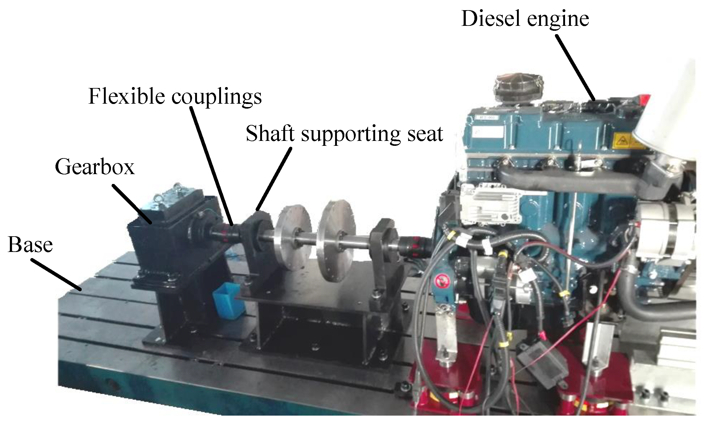
5.2. Case Study 2: Fault Diagnosis of Gearbox

The common faults of gears include local faults (pitting and teeth broken), distribution faults of worn types, and multiple coupled faults. Accurate fault identification is necessary for the safety of a mechanical system. In this section, a gearbox experimental dataset under different speeds was employed to validate the robustness of the proposed method. The test data were gathered on the gearbox platform shown in Figure 16, which consisted of a gearbox, a diesel engine, a bearing seat, a flexible coupling, a base, etc. The speed of the test system was controlled by electrical machinery. The gearbox contained two gears (pinion and wheel gear); their parameters are shown in

Table 1. Gear parameters of the test gearbox.

Gear Name	Teeth Number	Gear Modulus (mm)	Gear Pressure Angle (°)	Gear Material
Pinion gear	55	2	20	S45C
Wheel gear	75	2	20	S45C

. When the diesel engine ran, the Signal-Noise-Ratio was small. Therefore, the dataset validated the robustness to the noise of the proposed algorithm.

The gear dataset contained four kinds of faults: a coupled fault of wheel pit and pinion worn, a single pit of wheel, coupled fault of wheel broken and pinion worn, and a single worn of pinion. For convenience, the above four types of gear faults are named Type-2, Type-3, Type-4 and Type-5, respectively. In addition, the normal state of the gear is referred to as Type-1. Each fault type was tested under three different speeds. Note that the speed fluctuations also existed among different faults and the values of speeds are shown in

Table 2. Speeds of different fault types.

Speed	Type-1	Type-2	Type-3	Type-4	Type-5
Speed1 (rpm)	800	825	834	812	822
Speed2 (rpm)	820	849	850	842	845
Speed3 (rpm)	852	864	866	860	861

. The dataset of gearbox was averagely divided into two non-overlapping parts which were used as the training set and testing set.

The proposed method achieved excellent performance in its application to the gearbox fault diagnosis. The diagnosis results, compared with the original method by using different N_in, are displayed in Figure 17; notably, the paramater setting is the same as the bearing case. As seen in the figure, testing accuracies improved greatly. In addition, the non-montonicity phenomenon was significantly weak. The diagnosis accuracies with different percentages of training samples are shown in Figure 18. The experimental results show that the proposed method can effectively identify the gear health conditions with different fault types and severities, exhibiting a better performance than the original method.

To demonstrate the diagnosis information, the confusion matrix of the proposed method is displayed in Figure 19. Notably, the proposed method misclassifies 0.01% of testing samples of Type-2 as Type-1 and 0.02% of testing samples of Type-5 as Type-4. It is possible that the concurrent types were similar, making it more difficult to classify the two faults than other types.

6. Conclusions

This paper proposed a modified sparse filtering for machinery intelligent fault diagnosis by studying the nature of input dimension and overfitting. As illustrated in the experiments, the proposed method can effectively extract useful features from different fault types and achieve a higher diagnosis accuracy than the original method. The following major conclusions can be drawn.

• The interpretation of input dimension is studied based on the harmonic signal groups and bearing vibration signals. It can be concluded that the frequency resolution of weight matrix depends on input dimension.
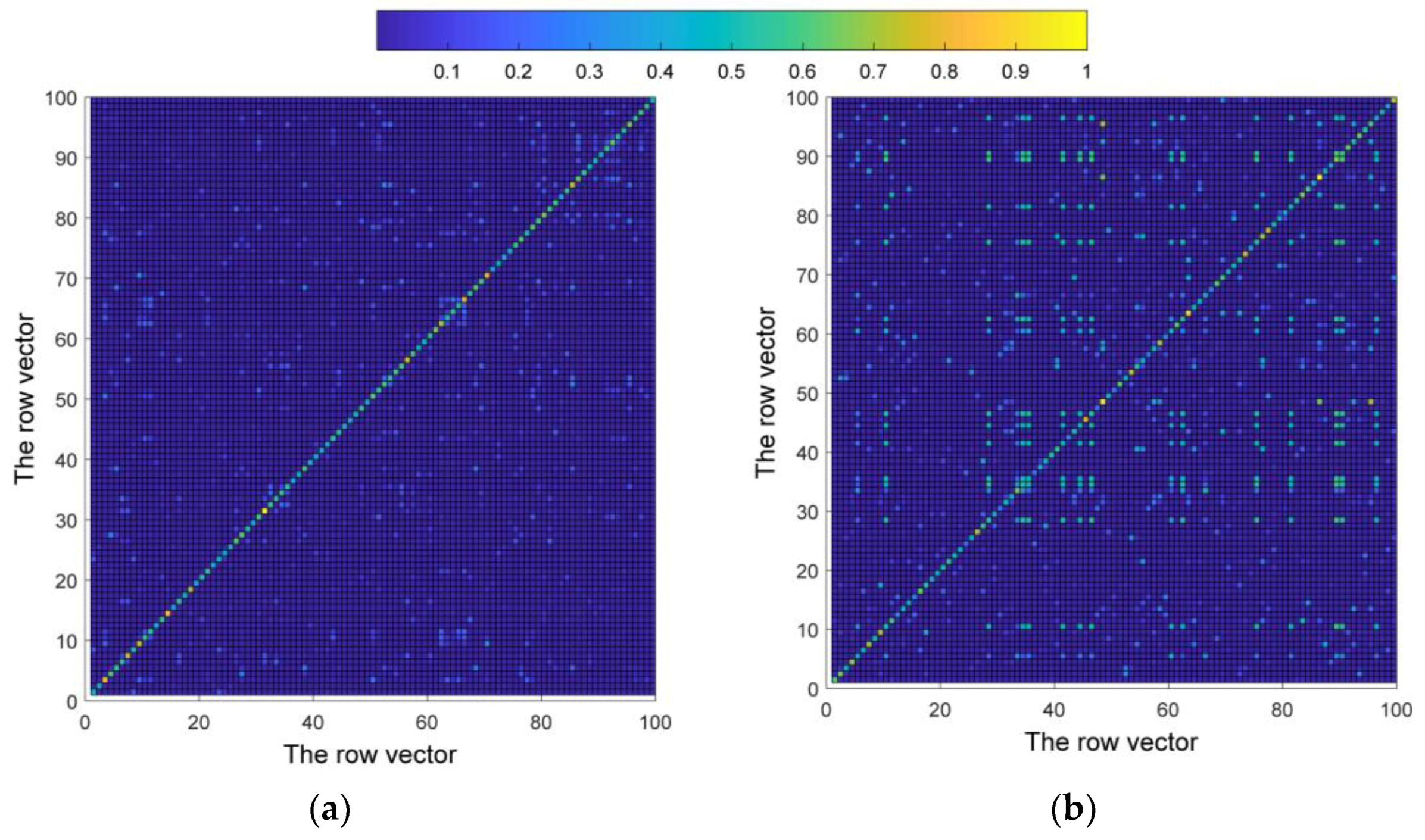
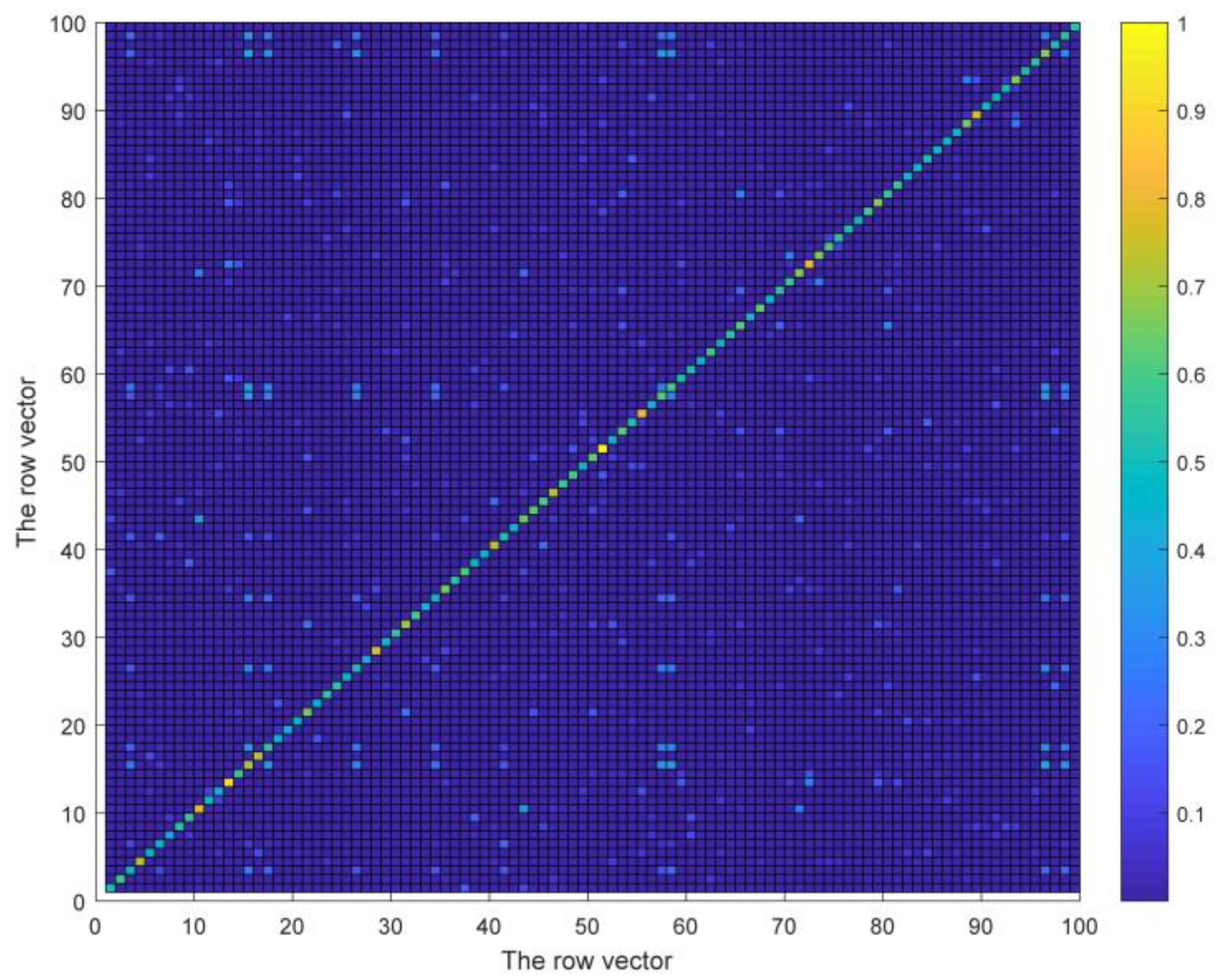
• The phenomenon known as non-monotonicity in this paper is explained as overfitting, which results from row vectors of weight matrix which are not orthogonal.
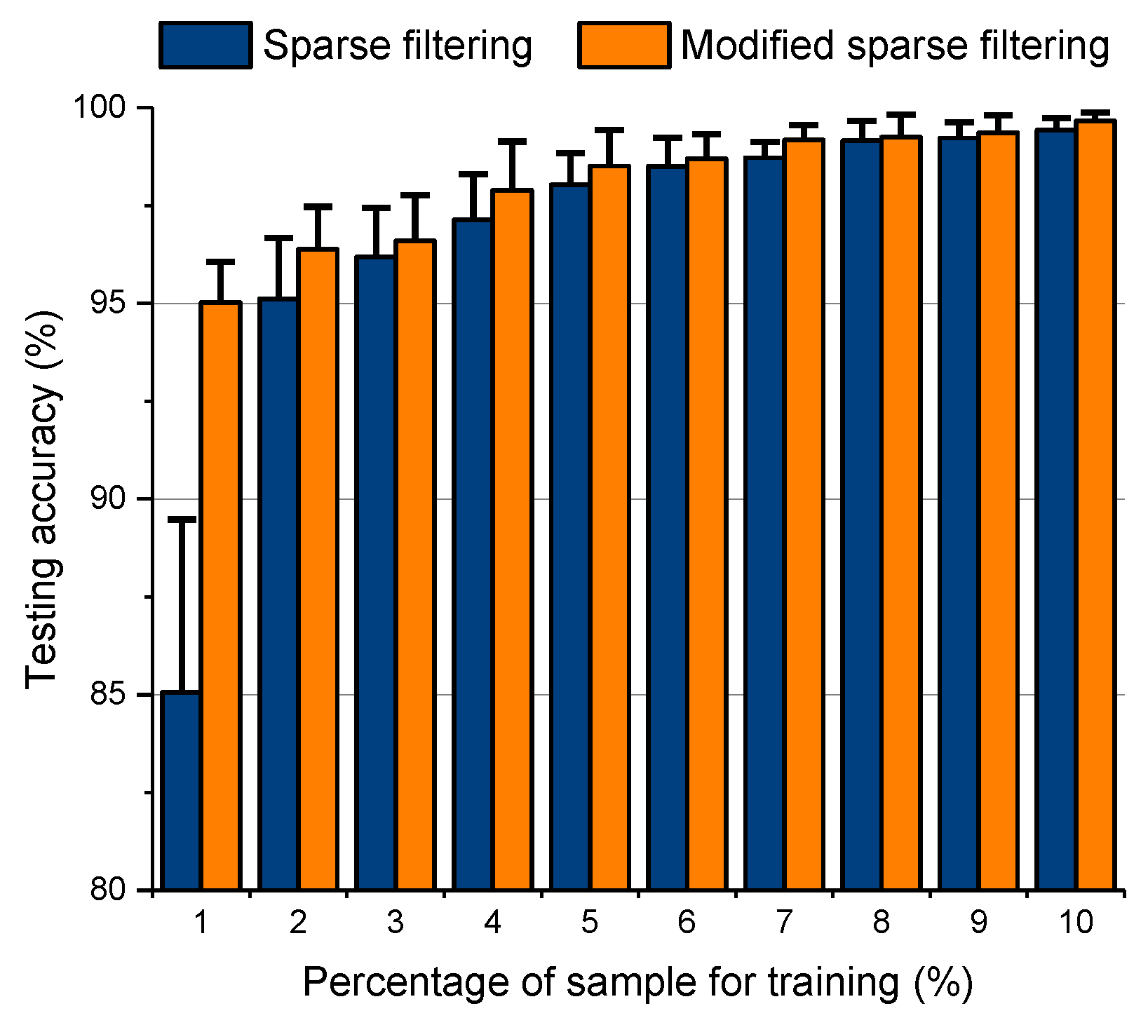
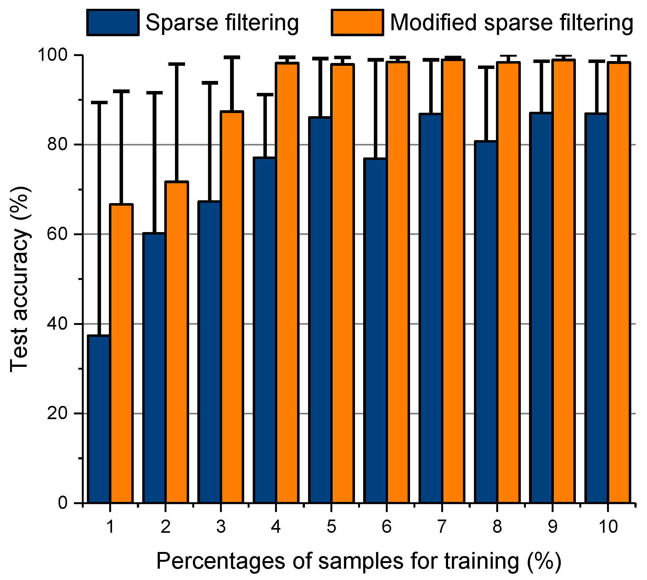
• The modified sparse filtering with a constraint term in the cost function can effectively handle the overfitting problem and eliminate the multi-correlation of the weight matrix.

References

1. Lu, S.; He, Q.; Dai, D.; Kong, F. Periodic fault signal enhancement in rotating machine vibrations via stochastic resonance. J. Vib. Control 2016, 22, 4227–4246. [Google Scholar] [CrossRef]
2. Yin, S.; Li, X.; Gao, H.; Kaynak, O. Data-based techniques focused on modern industry: An overview. IEEE Trans. Ind. Electron. 2015, 62, 657–667. [Google Scholar] [CrossRef]
3. Raj, A.S.; Murali, N. A novel application of lucy–richardson deconvolution: Bearing fault diagnosis. J. Vib. Control 2013, 21, 1055–1067. [Google Scholar] [CrossRef]
4. He, Q.; Ding, X. Sparse representation based on local time–frequency template matching for bearing transient fault feature extraction. J. Sound Vib. 2016, 370, 424–443. [Google Scholar] [CrossRef]
5. Jia, F.; Lei, Y.; Lin, J.; Zhou, X.; Lu, N. Deep neural networks: A promising tool for fault characteristic mining and intelligent diagnosis of rotating machinery with massive data. Mech. Syst. Signal Process. 2016, 72–73, 303–315. [Google Scholar] [CrossRef]
6. Guo, L.; Gao, H.; Huang, H.; He, X.; Li, S. Multifeatures fusion and nonlinear dimension reduction for intelligent bearing condition monitoring. Shock Vib. 2016, 2016, 4632562. [Google Scholar] [CrossRef]
7. Liu, H.; Li, L.; Ma, J. Rolling bearing fault diagnosis based on stft-deep learning and sound signals. Shock Vib. 2016, 2016, 6127479. [Google Scholar] [CrossRef]
8. Lu, S.; He, Q.; Zhao, J. Bearing fault diagnosis of a permanent magnet synchronous motor via a fast and online order analysis method in an embedded system. Mech. Syst. Signal Process. 2017. [Google Scholar] [CrossRef]
9. Sun, W.; An Yang, G.; Chen, Q.; Palazoglu, A.; Feng, K. Fault diagnosis of rolling bearing based on wavelet transform and envelope spectrum correlation. J. Vib. Control 2012, 19, 924–941. [Google Scholar] [CrossRef]
10. Sinha, J.K.; Elbhbah, K. A future possibility of vibration based condition monitoring of rotating machines. Mech. Syst. Signal Process. 2013, 34, 231–240. [Google Scholar] [CrossRef]
11. Ciabattoni, L.; Ferracuti, F.; Freddi, A.; Monteriu, A. Statistical spectral analysis for fault diagnosis of rotating machines. IEEE Trans. Ind. Electron. 2018, 65, 4301–4310. [Google Scholar] [CrossRef]
12. Cong, F.; Chen, J.; Dong, G.; Pecht, M. Vibration model of rolling element bearings in a rotor-bearing system for fault diagnosis. J. Sound Vib. 2013, 332, 2081–2097. [Google Scholar] [CrossRef]
13. Lu, W.; Liang, B.; Cheng, Y.; Meng, D.; Yang, J.; Zhang, T. Deep model based domain adaptation for fault diagnosis. IEEE Trans. Ind. Electron. 2017, 64, 2296–2305. [Google Scholar] [CrossRef]
14. Zhao, R.; Yan, R.; Wang, J.; Mao, K. Learning to monitor machine health with convolutional bi-directional lstm networks. Sensors 2017, 17, 273. [Google Scholar] [CrossRef] [PubMed]
15. Li, Y.; Kurfess, T.R.; Liang, S.Y. Stochastic prognostics for rolling element bearings. Mech. Syst. Signal Process. 2000, 14, 747–762. [Google Scholar] [CrossRef]
16. Liu, R.; Yang, B.; Zio, E.; Chen, X. Artificial intelligence for fault diagnosis of rotating machinery: A review. Mech. Syst. Signal Process. 2018, 108, 33–47. [Google Scholar] [CrossRef]
17. Paya, B.A.; Esat, I.; Badi, M. Artificial neural networks based fault diagnosis of rotating machinery using wavelet transforms as a preprocessor. Mech. Syst. Signal Process. 1997, 11, 751–765. [Google Scholar] [CrossRef]
18. Rafiee, J.; Arvani, F.; Harifi, A.; Sadeghi, M.H. Intelligent condition monitoring of a gearbox using artificial neural network. Mech. Syst. Signal Process. 2007, 21, 1746–1754. [Google Scholar] [CrossRef]
19. Liao, L.; Jin, W.; Pavel, R. Enhanced restricted boltzmann machine with prognosability regularization for prognostics and health assessment. IEEE Trans. Ind. Electron. 2016, 63, 7076–7083. [Google Scholar] [CrossRef]
20. Guo, X.; Chen, L.; Shen, C. Hierarchical adaptive deep convolution neural network and its application to bearing fault diagnosis. Measurement 2016, 93, 490–502. [Google Scholar] [CrossRef]
21. Janssens, O.; Slavkovikj, V.; Vervisch, B.; Stockman, K.; Loccufier, M.; Verstockt, S.; Van de Walle, R.; Van Hoecke, S. Convolutional neural network based fault detection for rotating machinery. J. Sound Vib. 2016, 377, 331–345. [Google Scholar] [CrossRef]
22. Lei, Y.; Zuo, M.J. Gear crack level identification based on weighted k nearest neighbor classification algorithm. Mech. Syst. Signal Process. 2009, 23, 1535–1547. [Google Scholar] [CrossRef]
23. Ngiam, J.; Koh, P.; Chen, Z.; Bhaskar, S.; Ng, A.Y. Sparse filtering. In Proceedings of the International Conference on Neural Information Processing Systems, Shanghai, China, 13–17 November 2011; pp. 1125–1133. [Google Scholar]
24. Zennaro, F.M.; Chen, K. Towards understanding sparse filtering: A theoretical perspective. Neural Netw. 2018, 98, 154–177. [Google Scholar] [CrossRef] [PubMed] [Green Version]
25. Yang, Z.; Jin, L.; Tao, D.; Zhang, S.; Zhang, X. Single-layer unsupervised feature learning with l2 regularized sparse filtering. In Proceedings of the IEEE China Summit & International Conference on Signal & Information Processing, Xi’an, China, 9–13 July 2014; IEEE: Piscataway, NJ, USA, 2014; pp. 475–479. [Google Scholar]
26. Dong, Z.; Pei, M.; He, Y.; Liu, T.; Dong, Y.; Jia, Y. Vehicle type classification using unsupervised convolutional neural network. In Proceedings of the 2014 22nd International Conference on Pattern Recognition, Stockholm, Sweden, 24–28 August 2014; IEEE: Piscataway, NJ, USA, 2014; pp. 172–177. [Google Scholar]
27. Wang, J.; Li, S.; Jiang, X.; Cheng, C. An automatic feature extraction method and its application in fault diagnosis. J. Vibroeng. 2017, 19, 2521–2533. [Google Scholar]
28. Lei, Y.; Jia, F.; Lin, J.; Xing, S.; Ding, S.X. An intelligent fault diagnosis method using unsupervised feature learning towards mechanical big data. IEEE Trans. Ind. Electron. 2016, 63, 3137–3147. [Google Scholar] [CrossRef]
29. Zhao, C.; Feng, Z. Application of multi-domain sparse features for fault identification of planetary gearbox. Measurement 2017, 104, 169–179. [Google Scholar] [CrossRef]
30. Jiang, G.-Q.; Xie, P.; Wang, X.; Chen, M.; He, Q. Intelligent fault diagnosis of rotary machinery based on unsupervised multiscale representation learning. Chin. J. Mech. Eng. 2017, 30, 1314–1324. [Google Scholar] [CrossRef]
31. Yang, Y.; Xiao, P.; Cheng, Y.; Zhang, X. Sparse filtering based intelligent fault diagnosis using ipso-svm. In Proceedings of the 36th Chinese Control Conference, Dalian, China, 26–28 July 2017; IEEE: Piscataway, NJ, USA, 2017; pp. 7388–7393. [Google Scholar]
32. Smith, E.C.; Lewicki, M.S. Efficient auditory coding. Nature 2006, 439, 978–982. [Google Scholar] [CrossRef] [PubMed]
33. Loparo, K. Case Western Reserve University Bearing Data Center. Available online: http://csegroups.case.edu/bearingdatacenter/pages/12k-drive-end-bearing-fault-data (accessed on 15 July 2013).
34. Masson, G.; Busettini, C.; Miles, F. Vergence eye movements in response to binocular disparity without depth perception. Nature 1997, 389, 283–286. [Google Scholar] [CrossRef] [PubMed]
35. Maaten, L.V.D.; Hinton, G. Visualizing data using t-sne. J. Mach. Learn. Res. 2008, 9, 2579–2605. [Google Scholar]
36. Zhang, W.; Li, C.; Peng, G.; Chen, Y.; Zhang, Z. A deep convolutional neural network with new training methods for bearing fault diagnosis under noisy environment and different working load. Mech. Syst. Signal Process. 2018, 100, 439–453. [Google Scholar] [CrossRef]
Figure 1. Architecture of sparse filtering.
Applsci 08 00906 g001
Figure 2. Diagnosis results of different input dimensions of the two harmonic signals groups.
Applsci 08 00906 g002
Figure 3. Relationship between the amplitudes of samples and the learned features.
Applsci 08 00906 g003
Figure 4. Diagnosis results using various input dimension of harmonic signals group of different frequencies.
Applsci 08 00906 g004
Figure 5. Relationship between the frequencies of samples and the learned features: (a) Nin = 200; (b) Nin = 100.
Applsci 08 00906 g005
Figure 6. Classification results of sparse filtering of various input dimensions.
Applsci 08 00906 g006
Figure 7. Selected weight vectors for the motor bearing dataset and the fitting vector by Gabor function: (a) Vectors in the time domain; (b) Fourier transforms.
Applsci 08 00906 g007
Figure 8. Results of WWT: (a) Nin = 100; (b) Nin = 200.
Applsci 08 00906 g008
Figure 9. Row vectors of W: (a) Vectors of Nin = 100 in the time domain; (b) Vectors of Nin = 100 in the frequency domain; (c) Vectors of Nin = 200 in the time domain; (d) Vectors of Nin = 200 in the frequency domain.
Applsci 08 00906 g009aApplsci 08 00906 g009b
Figure 10. Illustration of the proposed two-stage learning method.
Applsci 08 00906 g010
Figure 11. Diagnosis results using various input dimensions of modified and original sparse filtering.
Applsci 08 00906 g011
Figure 12. Diagnosis results obtained by different percentages of samples using modified and original sparse filtering.
Applsci 08 00906 g012
Figure 13. Visualization of features of validation dataset processed by t-SNE.
Applsci 08 00906 g013
Figure 14. Results of WWT of Nin = 200 using the proposed method.
Applsci 08 00906 g014
Figure 15. Row vectors of W: (a) Vectors of Nin = 200 in the time domain; (b) Vectors of Nin = 200 in the frequency domain.
Applsci 08 00906 g015
Figure 16. Platform of multi-fault gearbox.
Applsci 08 00906 g016
Figure 17. Diagnosis result using various input dimensions of modified and original sparse filtering.
Applsci 08 00906 g017
Figure 18. Diagnosis result trained by different percentages of samples using modified and original sparse filtering.
Applsci 08 00906 g018
Figure 19. Confusion matrix of the gear dataset.
Applsci 08 00906 g019