Dynamic Stiffness Effect of Mechanical Components on Gear Mesh Misalignment

Abstract

In this work, we propose a method that considers the dynamic elastic stiffness of mechanical components in a quasi-static condition, and we investigate this parameter’s effect on gear mesh misalignment. Unlike conventional approaches, which consider static stiffness only, the proposed method allows compensation of the dynamic response of the gearbox components under the quasi-static assumption, enabling more precise and practical gear design. A two-stage parallel gearbox is presented, designed, and numerically analyzed. The results demonstrate that the dynamic stiffness has a significant effect on gear misalignment and should, therefore, be carefully considered in the gear design process.

1. Introduction

The gear train is the most widely-used power transmission system, providing torque from rotary motion to other devices. The gear train’s most common use is in motor vehicles, such as automobiles, aeronautic vehicles, heavy equipment, and agricultural machines. The first step in the gearbox design process is to determine the macro-geometry of the gears, including the normal module, number of gear teeth, pressure angle, helix angle, face width, and center distance. 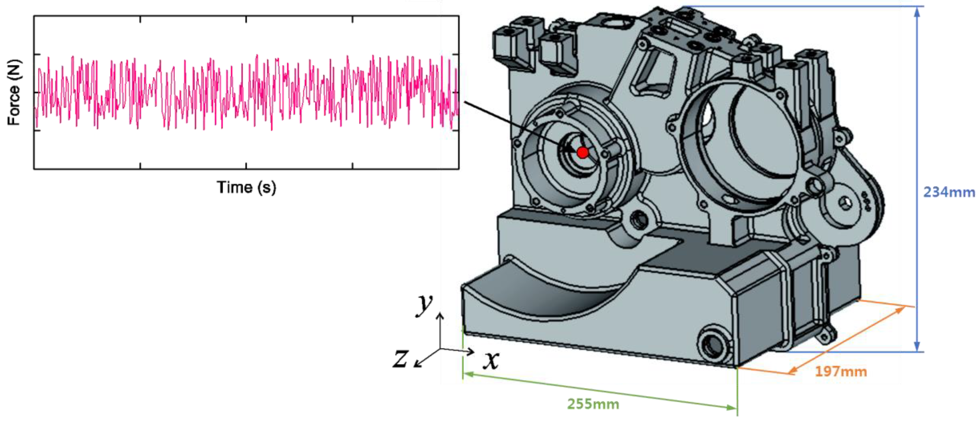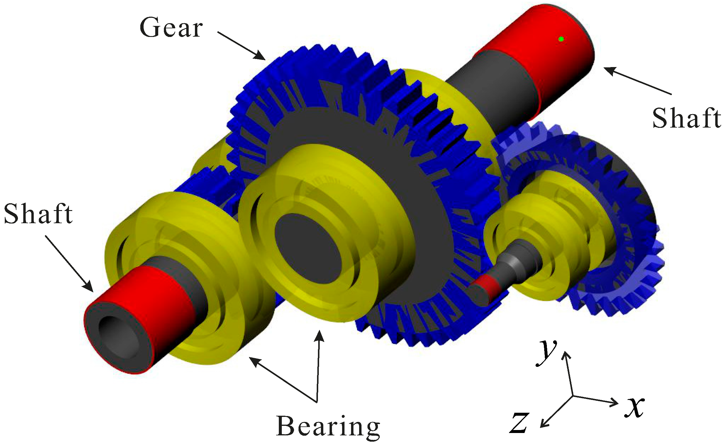The next step is to predict the gear mesh misalignment by considering the elastic stiffness of the shaft, bearing, and housing under a quasi-static condition [1,2]. However, the gear train is fundamentally a rotating machine, and, therefore, gears in the general operating condition cause dynamic loadings that are transmitted from the bearings to the housing structure. This causes time-varying interactions among the gearbox components, as can be seen in Figure 1. Therefore, the dynamic response of a geared rotor-bearing system should be considered for precise gear train design and analysis. Such designs have been studied extensively [3,4,5,6,7,8].

Recently, considering the housing stiffness has become recognized as important for controlling the gear train’s noise and vibration due to the use of lightweight gearbox housings in various vehicle industries for improved fuel efficiency. In such cases, various design codes encourage dynamic analysis to support the gearbox design procedure; however, such analyses incur heavy computational costs. Therefore, the initial steps, such as determining the macro- and micro-geometries of the gears and computing the gear mesh misalignment, generally continue to be performed under the static condition [9,10,11,12,13,14,15,16,17].

As a potential solution to this problem, we propose introducing a dynamic stiffness component that considers the relevant elastic and kinetic energies. This enables compensation of the dynamic features of the mechanical components in the quasi-static analysis. Under harmonic excitation, we can simply separate spatial and temporal variables in the dynamic equations of motion and compute the dynamic stiffness of the gearbox components as a quasi-static analysis. We can then compute the dynamic gear mesh misalignment and transmission error following the standard gear design procedure by simply replacing the static stiffness with the dynamic stiffness. Numerical investigations demonstrate that this simple modification of the typical gear design procedure can produce relevant differences in the gear mesh misalignment. We emphasize that the aim of this work is not a noise, vibration, and harshness (NVH) analysis, but rather a consideration of the dynamic stiffness effect in the conventional gear design process under a quasi-static condition.

Among the mechanical components, modeling the housing structure with the finite element (FE) method generally requires several numerical treatments. First, the degrees of freedom (DOFs) of the housing mesh surfaces where the bearings are located must be connected to the center of gravity of the bearing using rigid body elements (RBEs), which are also known as multi-point constraints [18,19,20,21]. In addition, simplifying the dynamic model of the FE housing, which has a tremendous number of DOFs, requires the use of reduced-order modeling (ROM) techniques [22,23,24,25,26,27,28,29,30,31,32,33]. Component mode synthesis (CMS) is currently the most popular ROM technique for dynamic systems [26,27,28,29,30,31]. The typical CMS method uses a small number of important and constraint modes to construct a reduced model that mathematically projects the displacement fields of the gearbox components onto modal coordinates. Thus, the accuracy level of the reduced system can be adjusted by adding (or eliminating) the desired number of modes. However, such modal projections require additional numerical treatments for application to the typical gear design process. To address this problem most efficiently, we use a Guyan reduction. This is a representative direct nodal condensation technique [23] that allows that the reduced matrices are only condensed into the physical coordinates, which means that the reduced matrices of Guyan reduction only have degrees of freedom (DOFs) related with the bearing center in the gearbox model.

In the following sections, we first introduce the gear design process and the formulations of the dynamic stiffness, including the reduced-order modeling. We then propose a numerical process of integrated gear design that considers the dynamic stiffness, and we investigate the effect of dynamic stiffness on gear mesh misalignment using a two-stage parallel gearbox example.

2. Summary of the Gearbox Design Process

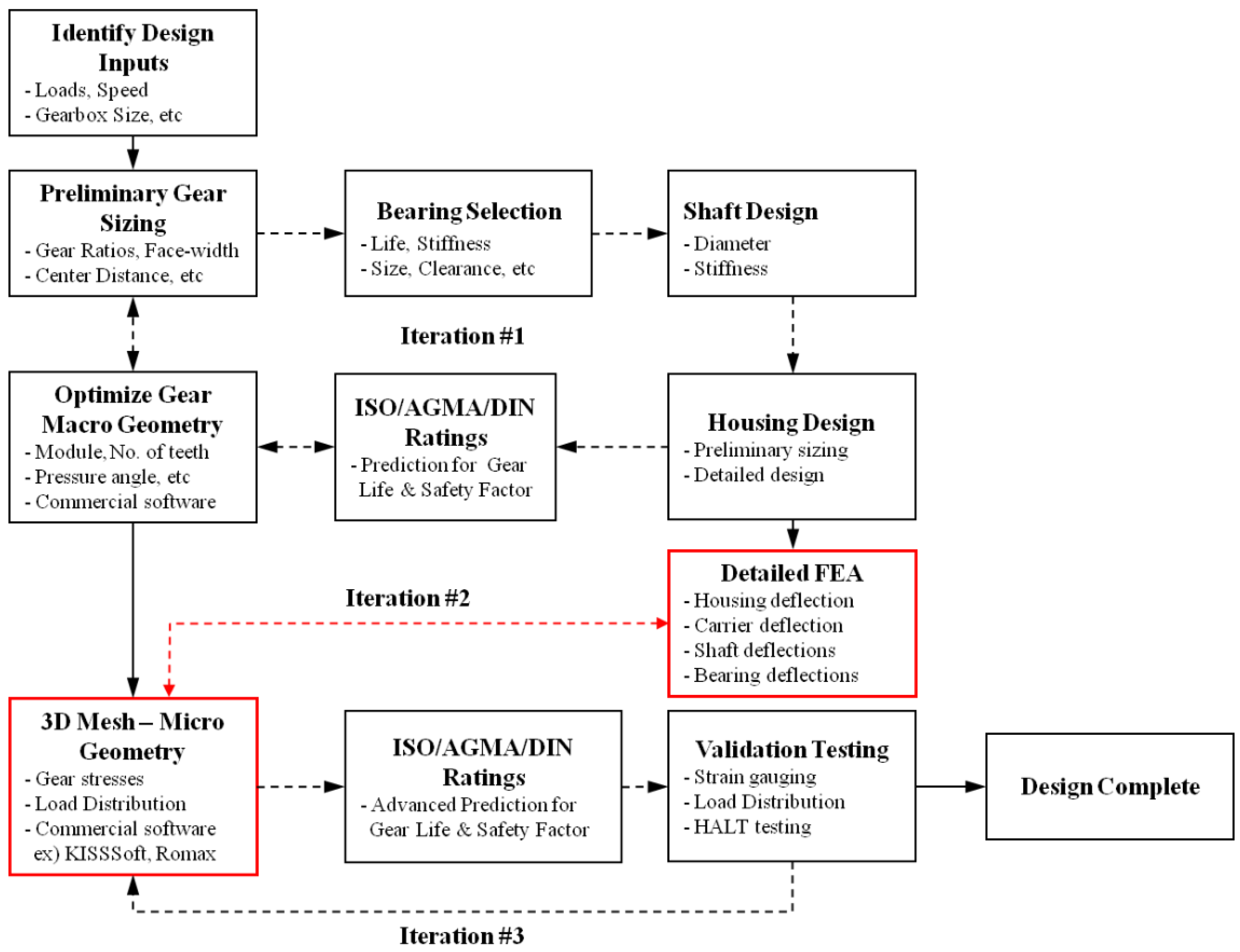
An optimal gearbox design process requires various advanced methods and iteration procedures, as can be seen in Figure 2. In the first step, a preliminary gear sizing is performed to meet the specified design requirements for the gearbox. Design parameters relevant to the size of the gearbox, such as the gear ratio, center distance, and gear face width, can be determined in this step.

In the second step, the gear macro-geometry is determined, including the normal module, number of gear teeth, pressure angle, helix angle, and profile shift coefficient, all of which are based on gear rating standards [10,11,12,13,14]. Bearings that can support the required gear loads are then selected, and shaft and housing are designed based on the gear macro-geometry.

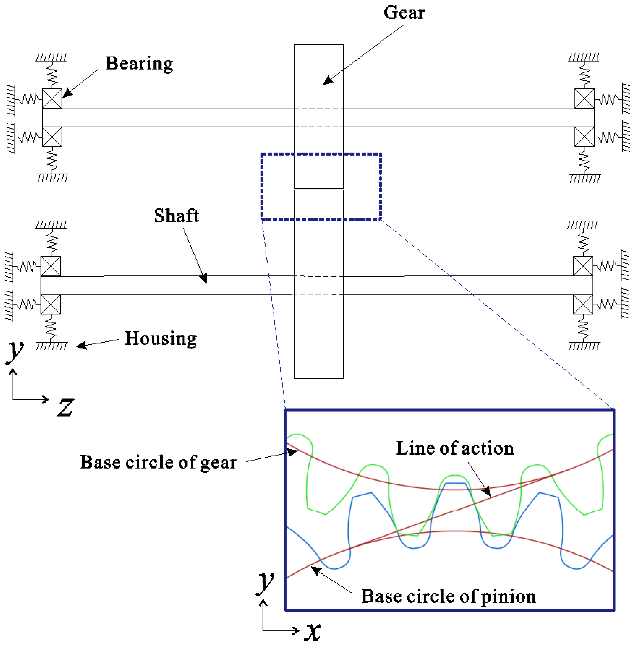
In the third step, the gear micro-geometry is determined, including the tip and root relief, lead slope, and crowning; these are based on the load distribution and transmission error analysis. Gear mesh misalignment between the meshed gears is a leading factor in the gear strength analysis, and the misalignment is iteratively computed using the shaft deflection and bearing deformation. The misalignment is then converted to displacement along the line of action on the gear mesh, as shown in Figure 3. A smaller mesh misalignment represents a more uniform load distribution on the gear mesh. The gear mesh misalignment in the line of action direction (Figure 3) is defined as:

$$F_{\beta X}=b \tan \phi , \phi ={\theta }_{skew}\cos {\alpha }_{wt}+{\theta }_{slope}$$

(1)

in which $F_{\beta X}$ is the gear mesh misalignment; $b$ is the face width; $\phi$ is the angle of gear mesh misalignment; ${\alpha }_{wt}$ is the working transverse pressure angle; and ${\theta }_{skew}$ and ${\theta }_{slope}$ are the angles of gear skew and slope, respectively.

From this gear mesh misalignment, we can compute the face load factor for contact stress which accounts for the effect of the load distribution over the face width on the gear contact stress. The definition of the face load factor is:

$$K_{H\beta }=\frac{\mathrm{Maximum} \mathrm{load} \mathrm{per} \mathrm{unit} \mathrm{face} \mathrm{width}}{\mathrm{Average} \mathrm{load} \mathrm{per} \mathrm{unit} \mathrm{face} \mathrm{width}}=\frac{\max \left(F/b\right)}{F_m/b}$$

(2)

where $K_{H\beta }$ is the face load factor, and $F$ and $F_m$ are the load at an arbitrary position of the tooth flank and the mean (average) load at the reference circle, respectively [10]. In engineering practice, the face load factor is computed as:

$$K_{H\beta }=\{\begin{array}{c}\sqrt{\frac{2F_{\beta Y}{c}_{\gamma \beta }}{F_m/b}},\mathrm{if}\frac{F_{\beta Y}{c}_{\gamma \beta }}{2F_m/b}\ge 1,\\ 1+\frac{F_{\beta Y}{c}_{\gamma \beta }}{2F_m/b},\mathrm{if} \mathrm{else},\end{array}$$

(3)

and then the effective gear mesh misalignment, denoted as $F_{\beta Y}$, is defined as:

$$F_{\beta Y}=F_{\beta X}-y_{\beta }$$

(4)

where $c_{\gamma \beta }$ is the mean value of the mesh stiffness per unit face width, and $y_{\beta }$ is the running-in allowance for a gear pair.

The gear mesh misalignment causes non-uniform load distribution along the face width in the plane of action, possibly resulting from gear elastic deflection, housing flexibility, and bearing deformation. As the most important factor in the gear strength rating, the face load factor must be equal to or greater than 1.0. A value of 1.0 is assumed to indicate that loads acting on gear tooth flanks are evenly distributed. As the value increases above 1.0, the load distribution on the gear tooth flanks becomes increasingly uneven [1,2]. This iteration procedure corresponds to Iteration #2 in the overall gear design process shown in Figure 2.

3. Gear Train Modeling Process with Dynamic Stiffness

This section presents the reduced-order modeling procedure for the gear train structure and introduces the definition of dynamic stiffness. Among the gear train components, the gears and bearings have been simply modeled using analytical and empirical techniques. However, the shaft and housing structural components are modeled using the finite element (FE) method. In particular, the FE method is the most popular approach to modeling housing structures with arbitrary and complicated geometries, and the approach is applied here via RomaxDESIGNER (R17) and KISSsoft (2017). This is the most popular gearbox design and analysis software used to consider the elastic behavior of the gearbox components in the design process [5,18,19].

Before modeling the FE housing, the initial positions of bearing center are first determined within the rigid body assumption (Figure 3) as:

$$q_0={\left[{(q_0^1)}^T{(q_0^2)}^T\cdots {(q_0^j)}^T\cdots {(q_0^{N_B})}^T\right]}^T, q_0^j=\left(\begin{array}{c}{x}_0^j\\ y_0^j\\ z_0^j\end{array}\right)$$

(5)

where $q_0$ is the initial position vector of the bearings, $q_0^j$ is the initial position of the $j$th bearing, and $N_B$ denotes the number of bearings (variables associated with bearings are denoted by the subscript $B$). The bearing center plays an important role in connecting the gearbox components, including the shaft, bearings, gears, and housing.

Using the initial position $q_0$ within the quasi-static condition, the following initial reaction forces of the bearings are computed as:

$$f_0={\left[{(f_0^1)}^T{(f_0^2)}^T\cdots {(f_0^j)}^T\cdots {(f_0^{N_B})}^T\right]}^T, f_0^j={(f_{x_0}^j f_{y_0}^j f_{z_0}^j T_{x_0}^j T_{y_0}^j T_{z_0}^j)}^T$$

(6)

where $f_0$ is the initial reaction force vector of the bearings; $f_0^j$ is the initial reaction force of the $j$th bearing; and $f$ and $T$ are the force and torque (moment) components, respectively. The initial reaction force, $f_0$, is then loaded into the gear train model at the initial bearing center, $q_0$, and the gear train deformation can be computed in the quasi-static condition. The bearing center is then updated according to the gear train deformation, which means that the bearing reaction force also changes. Therefore, the reaction force and bearing center location should be iteratively computed until these updated values are the same as the previous values of $q_{i+i}=q_i$ and $f_{i+i}=f_i$. This information is required to more accurately predict and compute gear mesh misalignment.

The linear equations of motion for the housing structure are then defined as:

$$M\ddot{U}(x,t)+C\dot{U}(x,t)+KU(x,t)=F(x,t)$$

(7)

where $M$, $C$, and $K$ are the mass, damping, and stiffness matrices of the FE housing structure, respectively; $\ddot{U}(x,t)$, $\dot{U}(x,t)$, $U(x,t)$, and $F(x,t)$ are the acceleration, velocity, displacement, and force vectors, respectively; and $x$ and $t$ are the space and time variables. Using the relations $U(x_i,t)=u{e}^{\pm jwt}$ and $F(x_i,t)=f{e}^{\pm jwt}$ with $j^2=-1$, Equation (7) is rewritten as:

$$K_{DS}\left(\omega \right) u=f,K_{DS}\left(\omega \right)=K-{\omega }^{2}M\pm j\omega C$$

(8)

where $\omega$ indicates the angular frequency (rad/s), and the dynamic stiffness, which contains the potential and kinetic energies, denoted as $K_{DS}\left(\omega \right)$ to distinguish it from the static stiffness $K$. The angular frequency component, $\omega$, of the dynamic stiffness is an unknown variable, and depends on the critical speed of the gear drivetrain under the operation conditions.

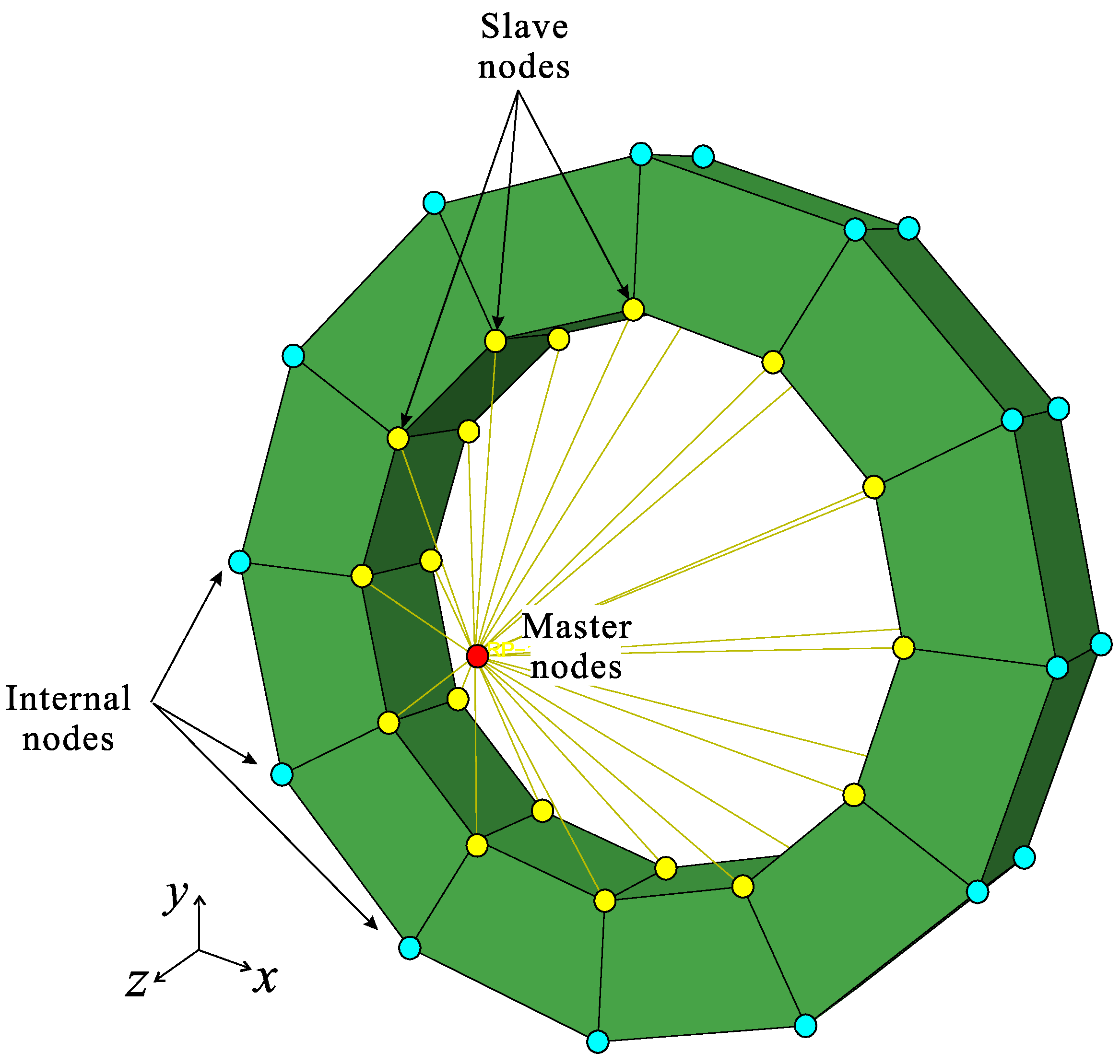
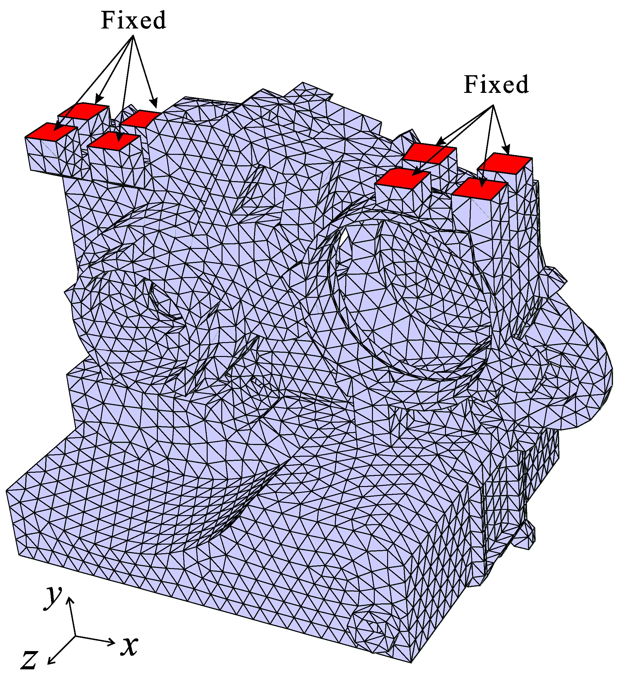
The housing structure is typically connected to the bearing center using a rigid body element (RBE), which is also known as a multipoint constraint [18,19,20,21]. Here, we use a conventional RBE formulation with the displacement constraints between master and slave DOFs determined by the master-slave, Lagrange multiplier, and penalty methods. In the master-slave method, DOFs are separated among internal, slave, and master nodes, as shown in Figure 4. In this case, the DOFs at the bearing centers are defined as masters, the DOFs constrained to the master DOF are slaves, and the other DOFs are internal. The components of Equation (8), except for the damping matrix, can then be rewritten as

$$M=\left[\begin{array}{ccc}{M}_{II}& M_{IS}& M_{IF}\\ M_{SI}& M_{SS}& M_{SF}\\ M_{FI}& M_{FS}& M_{FF}\end{array}\right],K=\left[\begin{array}{ccc}{K}_{II}& K_{IS}& K_{IF}\\ K_{SI}& K_{SS}& K_{SF}\\ K_{FI}& K_{FS}& K_{FF}\end{array}\right],u=\left(\begin{array}{c}{u}_I\\ u_S\\ u_F\end{array}\right),f=\left(\begin{array}{c}{f}_I\\ f_S\\ f_F\end{array}\right)$$

(9)

in which the internal, slave, and master DOFs are denoted by the subscripts $I$, $S$, and $F$, respectively. Here, we define a certain transformation matrix $A_{ij}^T$ as $A_{ji}$ ($A_{ij}^T=A_{ji}$). When we define the number of DOFs of the model as $N$, the numbers of the internal, slave, and master DOFs can be denoted as $N_I$, $N_S$, and $N_F$, respectively, and these typically have the following relation: $N_I>>N_S>N_F$ and $N=N_I+N_S+N_F$.

The master DOFs are typically independent, and the slave DOFs are physically dependent on the master DOFs. Considering these constraints, the slave DOFs can be presented using the Boolean matrix $B$ as:

$$u_S=B{u}_F$$

(10)

The Boolean matrix, $B$, is a $N_S$ by $N_F$ rectangular matrix. Using Equation (10), the displacement vector, $u$, is then transformed into the modified vector, $\widehat{u}$, by eliminating the slave DOFs:

$$u=T_S\widehat{u},T_S=\left[\begin{array}{cc}I& 0\\ 0& B\\ 0& I\end{array}\right],\widehat{u}=\left(\begin{array}{c}{u}_I\\ u_F\end{array}\right)$$

(11)

where $T_S$ is a transformation matrix, and $I$ is an identity matrix. Using Equations (9) and (11) in Equation (8), we obtain the following modified matrices:

$$\begin{array}{c}\widehat{M}=T_S^{T}M{T}_S=\left[\begin{array}{cc}{M}_{II}& {\widehat{M}}_{IF}\\ {\widehat{M}}_{FI}& {\widehat{M}}_{FF}\end{array}\right], \widehat{K}=T_S^{T}K{T}_S=\left[\begin{array}{cc}{K}_{II}& {\widehat{K}}_{IF}\\ {\widehat{K}}_{FI}& {\widehat{K}}_{FF}\end{array}\right], \\ \widehat{f}=T_S^{T}f=\left(\begin{array}{c}{f}_I\\ f_F+B^T{f}_S\end{array}\right)\end{array}$$

(12)

and these component matrices are then defined as:

$${\widehat{M}}_{IF}=M_{IS}B+M_{IF}, {\widehat{M}}_{IF}^T={\widehat{M}}_{FI}, {\widehat{M}}_{FF}=M_{FF}+M_{FS}B+B^T{M}_{SF}+B^T{M}_{SS}B$$

(13)

$${\widehat{K}}_{IF}=K_{IS}B+K_{IF}, {\widehat{K}}_{IF}^T={\widehat{K}}_{FI}, {\widehat{K}}_{FF}=K_{FF}+K_{FS}B+B^T{K}_{SF}+B^T{K}_{SS}B$$

(14)

This is a typical modeling result for an FE housing with RBEs.

Projecting the internal DOFs into the master DOFs at the bearing centers is the next step towards considering the housing effect in the gearbox design process. Using Equations (12) to (14), the linear static equations, which include $\widehat{K}\widehat{u}=\widehat{f}$, can be specifically presented as:

$$\left[\begin{array}{cc}{K}_{II}& {\widehat{K}}_{IF}\\ {\widehat{K}}_{FI}& {\widehat{K}}_{FF}\end{array}\right]\left(\begin{array}{c}{u}_I\\ u_F\end{array}\right)=\left(\begin{array}{c}{f}_I\\ f_F+B^T{f}_S\end{array}\right)$$

(15)

With the assumption of $f_I=0$, the well-known static constraint modes can be derived as:

$$u_I=\Psi u_F,\Psi =-K_{II}^{-1} {\widehat{K}}_{IF}$$

(16)

where $\Psi$ is a matrix of the static constraint modes that connects the internal DOFs ($u_I$) and the master DOFs ($u_F$) [22,23]. This connection is valid only for $f_F$, which implies that the external forces at the bearing center are dominant.

Using Equation (16), the modified displacement vector, $\widehat{u}$, can be presented simply by the master DOFs as:

$$\widehat{u}=T_I\overline{u},T_I=\left[\begin{array}{c}\Psi \\ I\end{array}\right],\overline{u}=u_F$$

(17)

Therefore, the mass and stiffness matrices in Equation (12) can be projected using $T_I$, as:

$$\overline{M}=T_I^T\widehat{M}{T}_I,\overline{K}=T_I^T\widehat{K}{T}_I,\overline{f}=T_I^T\widehat{f}$$

(18)

and can be detailed as:

$$\overline{M}={\widehat{M}}_{FF}+{\widehat{K}}_{FI}\Psi +{\Psi }^T {\widehat{K}}_{IF}+{\widehat{K}}_{FI}{K}_{II}^{-1}{M}_{II}{K}_{II}^{-1} {\widehat{K}}_{IF}, \overline{K}={\widehat{K}}_{FF}-{\widehat{K}}_{FI}{K}_{II}^{-1} {\widehat{K}}_{IF}$$

(19)

The condensed matrices, $\overline{M}$ and $\overline{K}$, are $N_F$ by $N_F$ matrices. The master DOFs, $u_F$, represent the bearing DOFs, which generally consist of six DOFs with three translations ($u_x,u_y,u_z$) and three rotations (${\theta }_x,{\theta }_y,{\theta }_z$). Therefore, $N_F$ is defined as $6N_B$ ($N_f=6N_B$).

The reduced matrices in Equation (19) are then represented as:

$$\overline{M}=\left[\begin{array}{cccc}{\overline{M}}_{B_1{B}_1}& & {\overline{M}}_{B_1{B}_j}& \\ & & & \\ {\overline{M}}_{B_i{B}_1}& & {\overline{M}}_{B_i{B}_j}& \\ & & & \end{array}\right], \overline{K}=\left[\begin{array}{cccc}{\overline{K}}_{B_1{B}_1}& & {\overline{K}}_{B_1{B}_j}& \\ & & & \\ {\overline{K}}_{B_i{B}_1}& & {\overline{K}}_{B_i{B}_j}& \\ & & & \end{array}\right] \mathrm{for} i \mathrm{and} j=1,2,\dots ,N_B$$

(20)

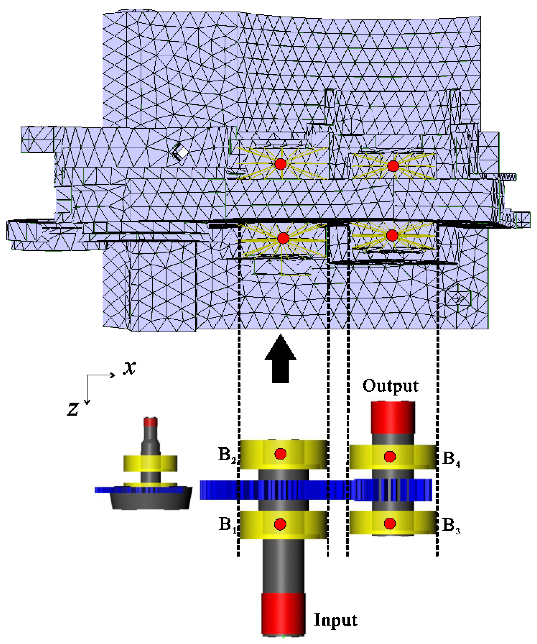
As an example, when the gearbox housing has four bearings ($N_B=4$), the size of the reduced matrices in Equation (20) are 24 by 24, and then the block diagonal matrices, ${\overline{M}}_{B_1{B}_1}$ and ${\overline{K}}_{B_1{B}_1}$, which are the mass and stiffness matrices of the $B_1$ bearing, are 6 by 6 matrices. Thus, the condensed matrices, $\overline{M}$ and $\overline{K}$, may be much smaller than the mass and stiffness matrices, $\widehat{M}$ and $\widehat{K}$. Using the reduced matrices, the dynamic stiffness in Equation (8) can be approximated as:

$${\overline{K}}_{DS}\left(\omega \right)\overline{u}=\overline{f},{\overline{K}}_{DS}\left(\omega \right)=\overline{K}-{\omega }^2\overline{M}\pm j\omega \overline{C}$$

(21)

In this work, we present the reduced-order FE modeling process with the dynamic stiffness for only the housing. However, the same process can be applied to other gear train components, such as the shafts and bearings. Hence, the general form of the dynamic stiffness can be defined as:

$${\overline{K}}_{DS}={\left[{\overline{K}}_{DS}\right]}_H+{\left[{\overline{K}}_{DS}\right]}_{Sh}+{\left[{\overline{K}}_{DS}\right]}_B$$

(22)

where the subscripts $H$ and $Sh$ represent terms associated with the housing and shaft, respectively.

In the typical gear design process, only the static stiffness, $\overline{K}$, is considered to compute the gear mesh misalignment [5]. However, the gear train is a rotary machine, and its housing is under dynamic loading in the operating condition, which means that precise predictions of the gear train behaviors require consideration of the system’s kinetic energy along with its potential energy. 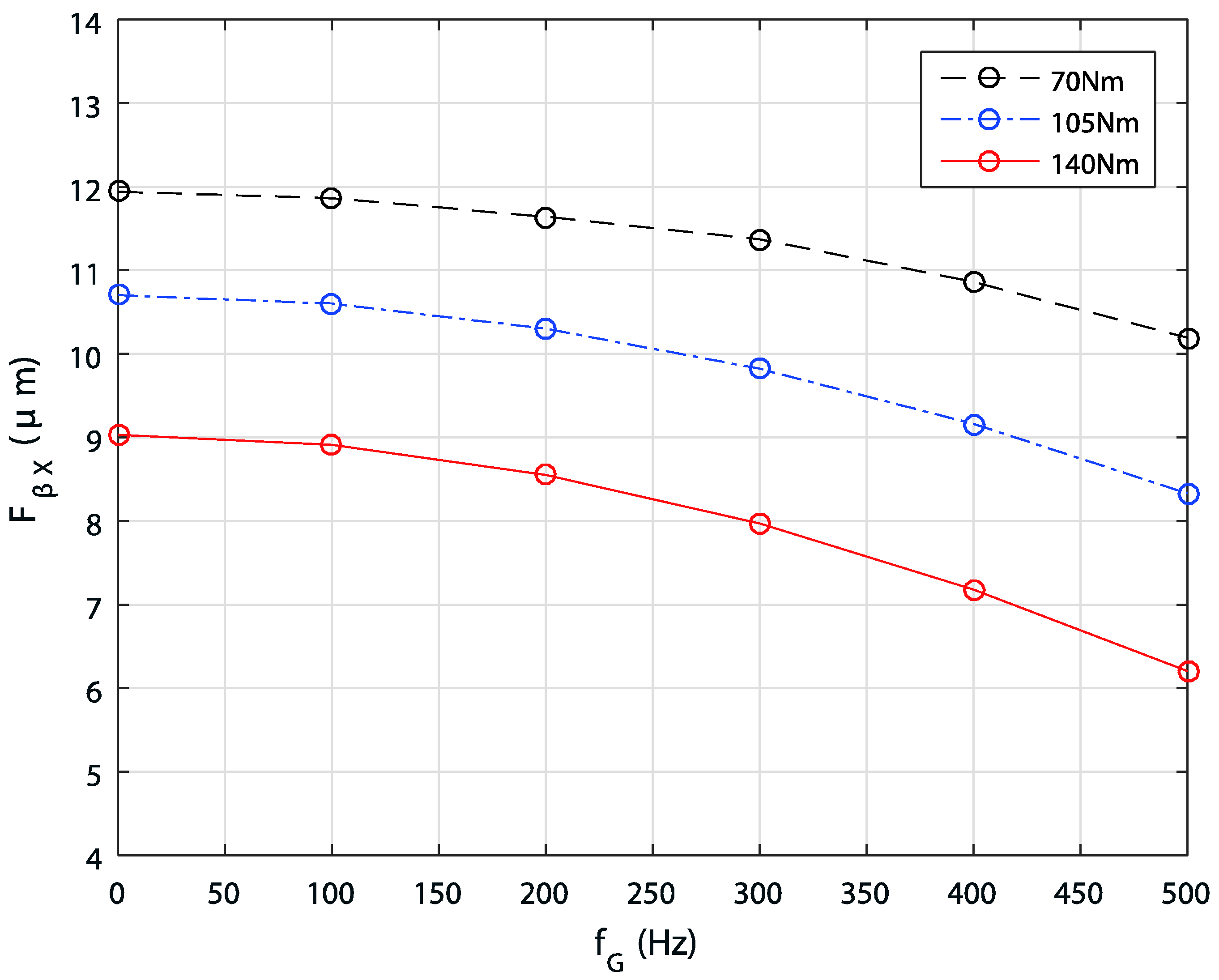Therefore, using the dynamic stiffness, ${\overline{K}}_{DS}\left(\omega \right)$, which contains both potential and kinetic energies, is a favorable approach for modeling the gearbox housing despite the imposed quasi-static condition. In particular, because the dynamic stiffness is a function of $\omega$, its effect becomes more significant in high-speed gear trains, such as those used in electric vehicles.

4. Gear Design Process Considering the Dynamic Stiffness

Here, we introduce a numerical gear design procedure for considering dynamic stiffness. In Step 1, using static analysis, the reaction force, $f_i$, at the bearing center is computed using the gear macro- and micro-geometries. In Step 2, $f_i$, is loaded onto the housing structure at the bearing center $q_i$. We can then compute the housing deformation using the dynamic stiffness in Equation (21). We should compute the angular frequency, $\omega$ (rad/s), first in Equation (21), which can be defined by the critical speed of the certain gearbox as:

$$\omega ={\omega }_G=2\pi f_G,f_G=N_G{f}_C$$

(23)

in which ${\omega }_G$ is the gear mesh angular frequency (rad/s), $f_G$ is the gear mesh frequency (Hz), $f_C$ is the gear rotating frequency (Hz), $N_G$ denotes the number of gear teeth, and the subscript $G$ indicates a term associated with the gear. The dynamic stiffness is then defined without the unknown variable as:

$${\overline{K}}_{DS}=\overline{K}-{\omega }_G^2\overline{M}\pm j{\omega }_G\overline{C}$$

(24)

Using the dynamic stiffness, except for the damping term in Equation (24), the displacement of the bearing center can be computed as:

$${\overline{u}}_{i+1}={\overline{K}}_{DS}^{-1}{\overline{f}}_i, {\overline{u}}_0=0, {\overline{f}}_0=f_0$$

(25)

and the bearing center is also updated as:

$$q_{i+1}=q_i+{\overline{u}}_{i+1}$$

(26)

Using the new bearing center, $q_{i+1}$, the updated reaction force, $f_{i+1}$, is computed again. This iteration procedure can stop when the following criteria are satisfied:

$$q_{i+1}-q_i=0, f_{i+1}-f_i=0$$

(27)

It implies that the bearing center and reaction force converge at certain values. Based on the results in Equation (27), the gear mesh misalignment, $F_{\beta X}$, in Equation (1) and the face load factor, $K_{H\beta }$, in Equation (3) can be computed and used in the gear design process.

A similar iteration process has been implemented in several commercialized software designs, including RomaxDesigner and KISSsoft [5,18,19]. However, these implementations apply only the static stiffness, $\overline{K}$, instead of the dynamic stiffness, ${\overline{K}}_{DS}$. This simple idea, using the dynamic stiffness,${\overline{K}}_{DS}$, can expose important differences in the gear mesh misalignment compared to the results obtained with static stiffness, as discussed in the next section.

5. Numerical Study

5.1. Gearbox Model

Herein, we use a general, industrial, two-stage parallel gearbox, as shown in Figure 5, to examine the effect of the dynamic stiffness of the elastic housing on gear mesh misalignment. The apparatus consists of a two-stage parallel spur gear set: One stage is for power transmission, and the other lubricates the pump drive.

In the gearbox model, the spur gears are modeled as the contact stiffness, and described in terms of macro and micro geometric parameters. The gear contact analysis includes a consideration of the gear mesh misalignment calculated from the system analysis as well as nonlinear tooth stiffness. The predicted contact location on the tooth flank influences the gear mesh force. In this work, all gear mesh forces and load distribution are considered and analyzed [1,2].

The rolling element bearings include internal geometries, such as the radial and axial clearance, number of rolling elements, and curvature of the raceways. This enables the bearings to have nonlinear stiffness. The stiffness matrix of each bearing is calculated by linearizing the nonlinear property of the bearing under the operating condition [1,2].

The elastic housing is simply modeled using tetrahedral solid elements (24,639 DOFs), as shown in Figure 6. The housing structure supports the gearbox at the four bearing centers, and is numerically modeled using the RBEs, as shown in Figure 7. Therefore, the FE model of the housing is reduced to a 24 by 24 (static or dynamic) stiffness matrix, and it is then assembled into shaft and bearing components. This dynamic stiffness modeling is performed by MATLAB in a personal computer (Intel Core (TM) i7-4770, 3.40 GHz CPU, 16 GB RAM). In this work, we consider an aluminum housing, and its material properties are presented in

Table 1. Material properties of housing.

Material	Young’s Modulus ($\mathit{E}$)	Poisson’s Ratio ($\mathit{\upsilon }$)	Density ($\mathit{\rho }$)
Aluminum	68 GPa	0.36	2700 kg/m3

. We also use a standard alloy special steel (18CrMo4) for the gears and shafts. Details of the input and output gears are presented in

Table 2. Specifications of gear pair.

Parameters	Unit	Input Gear	Output Gear
Normal module	mm	3	3
Pressure angle	deg.	20	20
Center distance	mm	71	71
Number of teeth	-	50	21
Face width	mm	13	15
Profile shift coefficient	-	−0.0616	0.0616
Gear quality (ISO 1328)	-	4	4
Material type	-	18CrMo4	18CrMo4
Young’s modulus ($E$)	GPa	206	206
Density ($\rho$)	kg/m3	7830	7830
Poisson’s ratio ($\upsilon$)	-	0.3	0.3

.

5.2. Numerical Results and Discussion

In this numerical study, the applied torque and gear mesh frequency are considered as the main variables. To predict the characteristics of the gearbox according to the torque change, the applied torque was set at three different levels: 70, 105, and 140 Nm, which are defined as 50, 75, and 100% of the nominal torque of 140 Nm. In addition, the gear mesh frequency, which plays a main role in the dynamic stiffness in Equation (21), was investigated in six cases: 0, 100, 200, 300, 400, and 500 Hz. The maximum gear mesh frequency, 500 Hz, is computed from Equation (23) based on an input speed of 600 rpm, which is the maximum input speed of the gearbox. These parameters are summarized in

Table 3. Numerical cases.

Parameters	Cases
Applied torque (Nm)	70, 105, 140
Gear mesh frequency (Hz)	0 (static stiffness), 100, 200, 300, 400, 500

. The first case of the dynamic stiffness at 0 Hz implies a static stiffness, from Equation (21), unlike the other cases. We first compute the static deflections of the shafts, gears, and bearings, considering the housing flexibility. The gear mesh misalignment, face load factor, transmission error, and contact pattern on the gear mesh are also predicted. Figure 8 presents the changing gear mesh misalignment, $F_{\beta X}$, with respect to the applied torque and gear mesh frequency. The numerical results show that $F_{\beta X}$ decreases when the applied torque and the gear mesh frequency increase. In particular, we investigated the specific gear mesh misalignments, $F_{\beta X}$, of the components, and the results are summarized in

Table 4. Gear mesh misalignments, $F_{\beta X}$, of the components in relation to applied torque when using static stiffness ($f_G$= 0 Hz).

Applied Torque	Components	Input Gear (μm)	Output Gear (μm)
70 Nm	Shaft	−6.696 × 10−2	−4.311 × 10−2
	Bearing	1.180 × 101	−4.481 × 10−1
	Housing	2.191 × 100	−1.493 × 100
105 Nm	Shaft	−6.674 × 10−2	−3.801 × 10−2
	Bearing	1.023 × 101	−3.517 × 10−1
	Housing	2.455 × 100	−1.548 × 100
140 Nm	Shaft	−6.781 × 10−2	−3.062 × 10−2
	Bearing	8.181 × 100	−2.592 × 10−1
	Housing	2.830 × 100	−1.621 × 100

. The numerical results imply that $F_{\beta X}$ of the input gear is much larger than $F_{\beta X}$ of the output gear, and that $F_{\beta X}$ of the bearing accounts for approximately 80% of the total gear mesh misalignment. In addition, as the applied torque increased from 70 to 140 Nm, the total amount of $F_{\beta X}$ decreases because $F_{\beta X}$ of the bearing dramatically decreased. This result can be attributed to an increase in the reaction forces acting on the bearing with increasing torque. This leads directly to larger bearing deformation, and we can expect larger reaction moments between the rolling elements, such as the balls, rollers, and raceway. This situation can result in a relative reduction of the bearing misalignment.

This tendency is clearly apparent when comparing the contact pattern of the gear tooth flanks provided in Figure 9. Figure 9a,b has similar contact patterns, and the load can be seen to be distributed unevenly along the face width. However, the contact pattern of the dynamic stiffness with $f_g=500$ Hz is relatively more even than the contact pattern of the static stiffness with $f_g=0$ Hz. The maximum and average normal forces in the contact patterns are summarized in

Table 5. Maximum and average normal forces in contact patterns when torque is 140 Nm.

Normal Force	Units	Static Stiffness	Dynamic Stiffness
		0 Hz	300 Hz	500 Hz
Maximum	N/mm	340	330	320
Average	N/mm	283	280	281

. The face load factor, $K_{H\beta }$, that is defined in Equation (2) also decreases when the applied torque and the gear mesh frequency increase, as shown in Figure 10.

The differences in $F_{\beta X}$ and $K_{H\beta }$ caused by the dynamic stiffness effect may lead to changes in the peak-to-peak gear transmission error (PPTE), which is a main source of whine noise. Figure 11 compares the PPTE of the three different gear mesh frequencies when the applied torque is 140 Nm. Although the differences are not significant, the effect of the dynamic stiffness becomes much more important when we consider a high-speed gear train, such as what is used in electric vehicles.

6. Conclusions

This study demonstrated that considering the elastic stiffness of mechanical components, such as housings, bearings, and shafts, in the gear design process can lead to significant effects on gear mesh misalignment. In particular, unlike the conventional approach of considering the static stiffness only, we consider the dynamic stiffness along with the gear mesh frequency. This approach is appropriate because in normal operation conditions a gear train is fundamentally under dynamic loading. In this work, we proposed a simple design process to compute the gear mesh misalignment by considering the dynamic stiffness under a quasi-static condition and examined the impact of this consideration using a two-stage parallel gearbox. We found that employing the dynamic stiffness can lead to different design results in terms of misalignment, face load factor, contact pattern, and transmission error when compared to cases in which only the static stiffness was considered. In particular, differences in the gear mesh misalignment between cases using static or dynamic stiffness increase with higher gear mesh frequency, and also larger applied torque. This numerical study allows us to conclude that, for improved design results, the dynamic stiffness should be considered in the gear design process because it can directly lead to improved tooth modification and whine noise control. We emphasize again that the aim of this work was not an NVH analysis, but was rather a consideration of the dynamic stiffness effect in the gear design process under a quasi-static condition. In this work, we only focused on the numerical investigation of the dynamic stiffness effects, but those should be carefully validated with the experimental study in the near future, and the NVH issues should also be tackled using the proposed dynamic stiffness approaches.

References

1. Park, Y.J.; Lee, G.H.; Song, J.S.; Nam, Y.Y. Characteristic analysis of wind turbine gearbox considering non-torque loading. J. Mech. Des. 2013, 135, 044501. [Google Scholar] [CrossRef]
2. Park, Y.J.; Kim, J.G.; Lee, G.H.; Shim, S.B. Load sharing and distributed on the gear flank of wind turbine planetary gearbox. J. Mech. Sci. Technol. 2015, 29, 309–316. [Google Scholar] [CrossRef]
3. Özgüven, H.N.; Houser, D.R. Mathematical models used in gear dynamics—A review. J. Sound Vib. 1988, 121, 383–411. [Google Scholar] [CrossRef]
4. Seybert, A.F.; Wu, T.W.; Wu, X.F.; Oswald, F.B. Acoustical analysis of gear housing vibration. In Proceedings of the AHS and Royal Aeronautical Society, Technical Specialists’ Meeting on Rotorcraft Acoustics, Philadelphia, PA, USA, 1 January 1991. [Google Scholar]
5. Harris, O.J.; Douglas, M.; James, B.M.; Wooley, A.M.; Lack, L.W. Predicting the effects of transmission housing flexibility and bearing stiffness on gear mesh misalignment and transmission error. In Proceedings of the 2nd MSC Worldwide Automotive Conference, Dearborn, MI, USA, January 2000. [Google Scholar]
6. Abbes, M.S.; Fakhfakh, T.; Haddar, M.; Maalej, A. Effect of transmission error on the dynamic behaviour of gearbox housing. Int. J. Adv. Manuf. Technol. 2007, 34, 211. [Google Scholar] [CrossRef]
7. Pears, J.; Smith, A.; Platten, M.; Abe, T.; Wilson, B.; Cheng, Y.; Felice, M. Predicting variation in the NVH characteristics of an automatic transmission using a detailed parametric modelling approach. SAE Tech. Pap. 2007. [Google Scholar] [CrossRef]
8. James, B.M.; Hofmann, A. Simulating and reducing noise excited in an EV powertrain by a switched reluctance machine. SAE Tech. Pap. 2014. [Google Scholar] [CrossRef]
9. Radzevich, S.P. Dudley’s Handbook of Practical Gear Design and Manufacture; CRC Press: Boca Raton, FL, USA, 2016. [Google Scholar]
10. International Organization for Standardization. Calculation of Load Capacity of Spur and Helical Gears; ISO 6336:2007; ISO: Geneva, Switzerland, 2006. [Google Scholar]
11. International Organization for Standardization. Calculation of Load Capacity of Bevel Gears; ISO 10300:2001; ISO: Geneva, Switzerland, 2001. [Google Scholar]
12. International Organization for Standardization. Calculation of Load Capacity of Worm Gears; ISO/TS 14521:2010; ISO: Geneva, Switzerland, 2010. [Google Scholar]
13. American Gear Manufacturers Association. Fundamental Rating Factors and Calculation Methods for Involute Spur and Helical Gear Teeth; American Gear Manufacturers Association: Alexandria, VA, USA, 1994. [Google Scholar]
14. Deutsches Institut fuer Normung EV. 3990—Calculation of Load Capacity of Cylindrical Gears; DIN: Berlin, Germany, 1987. [Google Scholar]
15. Pedrero, J.I.; Pleguezuelos, M.; Artés, M.; Antona, J.A. Load distribution model along the line of contact for involute external gears. Mech. Mach. Theory 2010, 45, 780–794. [Google Scholar] [CrossRef]
16. Li, S. Effects of misalignment error, tooth modifications and transmitted torque on tooth engagements of a pair of spur gears. Mech. Mach. Theory 2015, 83, 125–136. [Google Scholar] [CrossRef]
17. Roda-Casanova, V.; Sanchez-Marin, F.T.; Gonzalez-Perez, I.; Iserte, J.L.; Fuentes, A. Determination of the ISO face load factor in spur gear drives by the finite element modeling of gears and shafts. Mech. Mach. Theory 2013, 65, 1–3. [Google Scholar] [CrossRef]
18. Montgomery, J. Methods for modeling bolts in the bolted joint. In Proceedings of the ANSYS User’s Conference, Canonsburg, PA, USA, 22–24 April 2002. [Google Scholar]
19. Romax Technology Ltd. Manual RU; Romax Technology Ltd.: Nottingham, UK, 2003. [Google Scholar]
20. Hibbitt, Karlsson, Sorensen. ABAQUS/Explicit: User’s Manual; Hibbitt, Karlsson and Sorenson Incorporated: Providence, RI, USA, 2001. [Google Scholar]
21. MSC Nastran. Basic Dynamic Analysis User’s Guide; MSC Software Corporation: Santa Ana, CA, USA, 2004. [Google Scholar]
22. Turner, M.J. Stiffness and deflection analysis of complex structures. J. Aero. Sci. 1956, 23, 805–823. [Google Scholar] [CrossRef]
23. Guyan, R.J. Reduction of stiffness and mass matrices. AIAA J. 1965, 3, 380. [Google Scholar] [CrossRef]
24. O’Callahan, J.C. A procedure for an improved reduced system (IRS) model. In Proceedings of the 7th International Modal Analysis Conference, Las Vegas, NV, USA, 30 January–2 February 1989; pp. 17–21. [Google Scholar]
25. Friswell, M.I.; Garvey, S.D.; Penny, J.E. Model reduction using dynamic and iterated IRS techniques. J. Sound Vib. 1995, 186, 311–323. [Google Scholar] [CrossRef]
26. Hurty, W.C. Dynamic analysis of structural systems using component modes. AIAA J. 1965, 3, 678–685. [Google Scholar] [CrossRef]
27. Craig, R.; Bampton, M. Coupling of substructures for dynamic analyses. AIAA J. 1968, 6, 1313–1319. [Google Scholar]
28. MacNeal, R.H. A hybrid method of component mode synthesis. Comput. Struct. 1971, 1, 581–601. [Google Scholar] [CrossRef]
29. Park, K.C.; Park, Y.H. Partitioned component mode synthesis via a flexibility approach. AIAA J. 2004, 42, 1236–1245. [Google Scholar] [CrossRef]
30. Kim, J.G.; Lee, P.S. An enhanced Craig–Bampton method. Int. J. Numer. Meth. Eng. 2015, 103, 79–93. [Google Scholar] [CrossRef]
31. Kim, J.G.; Boo, S.H.; Lee, P.S. An enhanced AMLS method and its performance. Comput. Methods Appl. Mech. Eng. 2015, 287, 90–111. [Google Scholar] [CrossRef]
32. Kim, J.G.; Markovic, D. High-fidelity flexibility-based component mode synthesis method with interface degrees of freedom reduction. AIAA J. 2016, 54, 3619–3631. [Google Scholar] [CrossRef]
33. Kim, J.G.; Park, Y.J.; Lee, G.H.; Kim, D.N. A general model reduction with primal assembly in structural dynamics. Comput. Methods Appl. Mech. Eng. 2017, 324, 1–28. [Google Scholar] [CrossRef]
Figure 1. Example of gearbox housing under gear-induced dynamic loading at a bearing center.
Applsci 08 00844 g001
Figure 2. Typical gearbox design procedure (Radzevich, 1951).
Applsci 08 00844 g002
Figure 3. Schematic of gearbox with transverse line of action between the meshed gears.
Applsci 08 00844 g003
Figure 4. One rigid body element (RBE), where the red dot represents a master node, yellow dots represent slave nodes, and blue dots represent internal nodes.
Applsci 08 00844 g004
Figure 5. A two-stage parallel gear.
Applsci 08 00844 g005
Figure 6. FE housing model.
Applsci 08 00844 g006
Figure 7. Placement of gear assembly in FE housing.
Applsci 08 00844 g007
Figure 8. Gear mesh misalignment, F β X , in relation to torque and gear mesh frequency.
Applsci 08 00844 g008
Figure 9. Comparison of contact patterns when torque is 140 Nm. (a) f G = 0 Hz (static stiffness) and (b) f g = 500 Hz (dynamic stiffness).
Applsci 08 00844 g009
Figure 10. Face load factor, K H β , in relation to torque and gear mesh frequency.
Applsci 08 00844 g010
Figure 11. Transmission error depending on gear mesh frequency when torque is 140 Nm.
Applsci 08 00844 g011