Neural Prediction of Tunnels’ Support Pressure in Elasto-Plastic, Strain-Softening Rock Mass


Abstract
:Featured Application
Abstract
1. Introduction
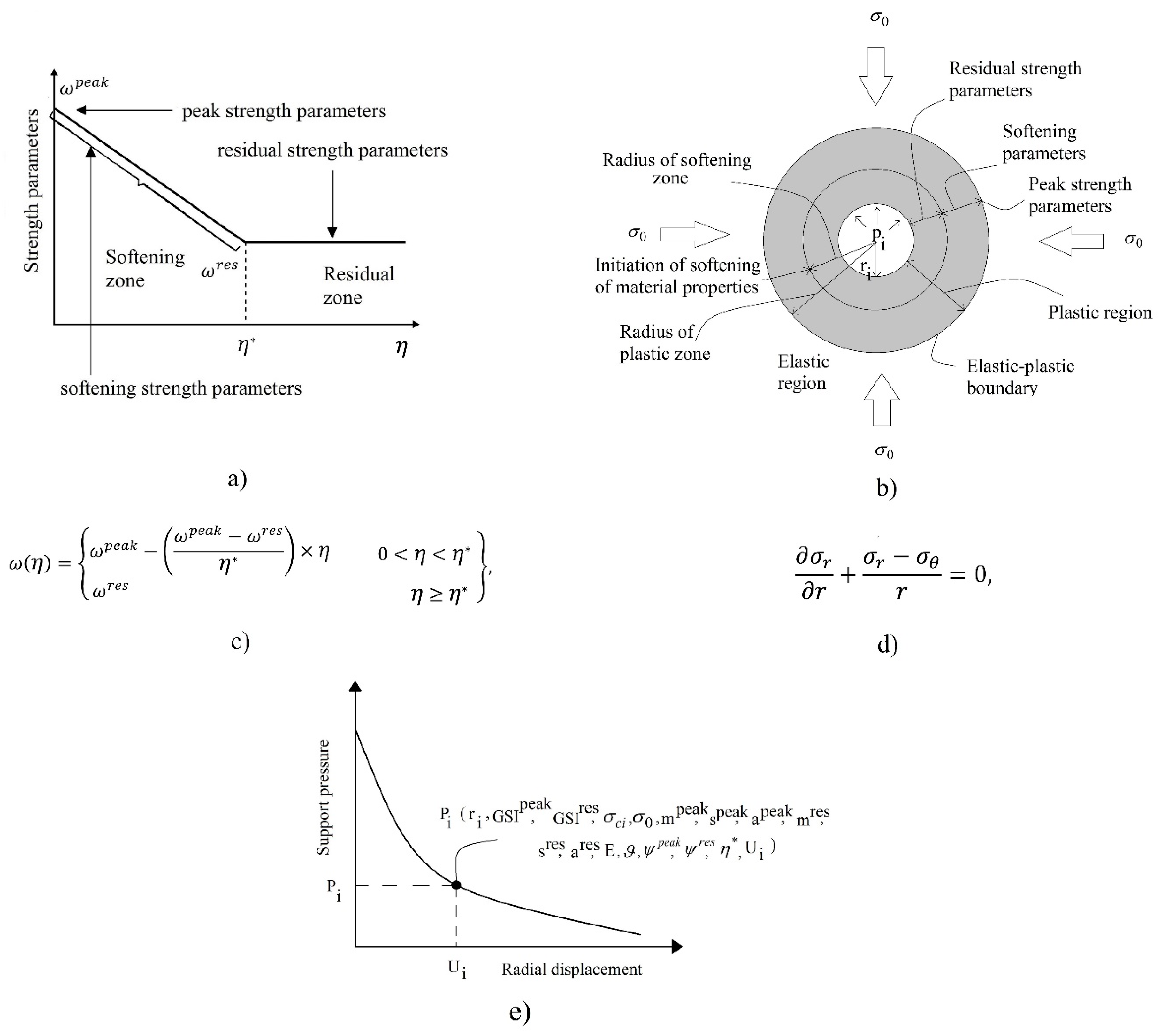
2. Methodology
Data Acquisition
3. Performance Evaluation
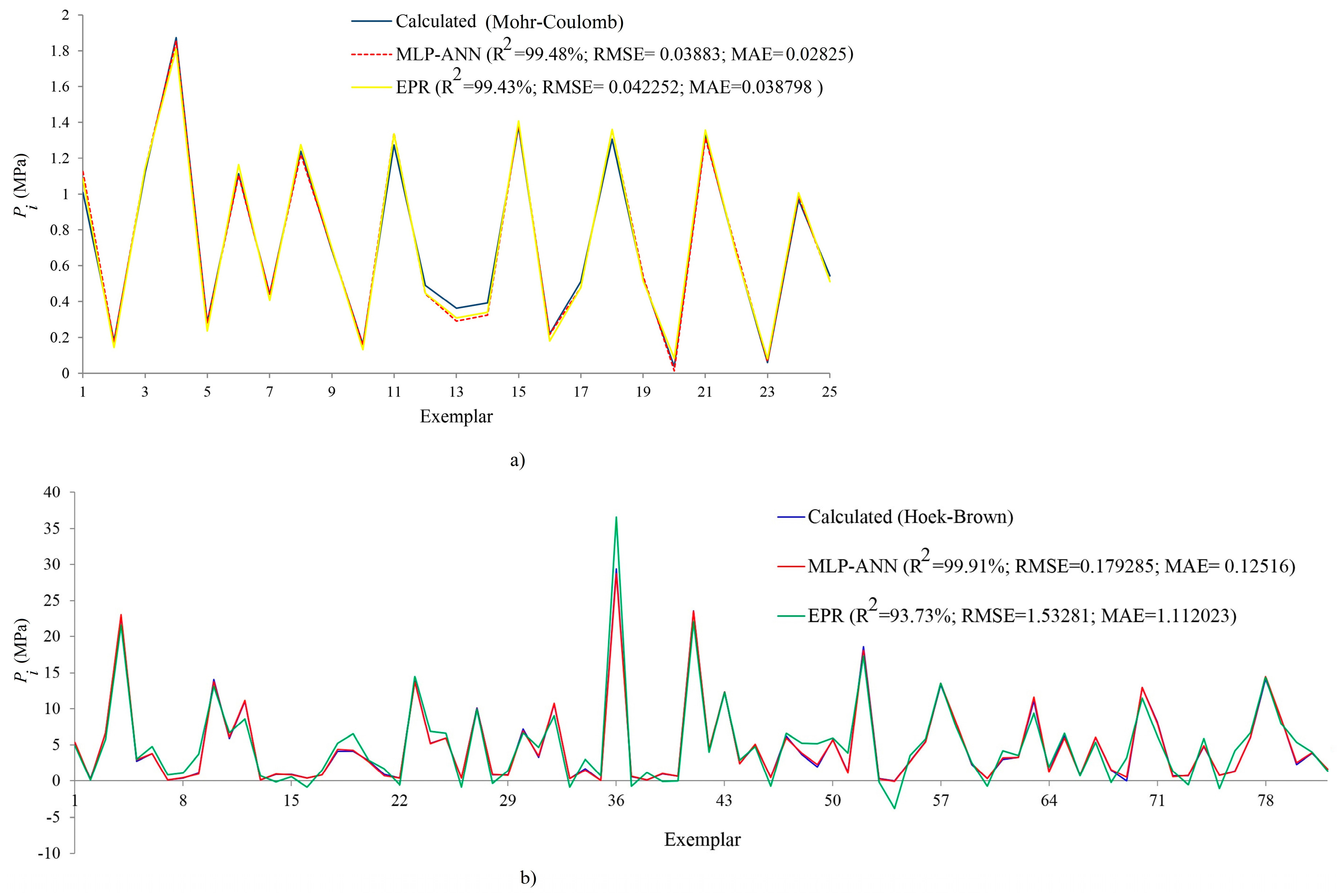
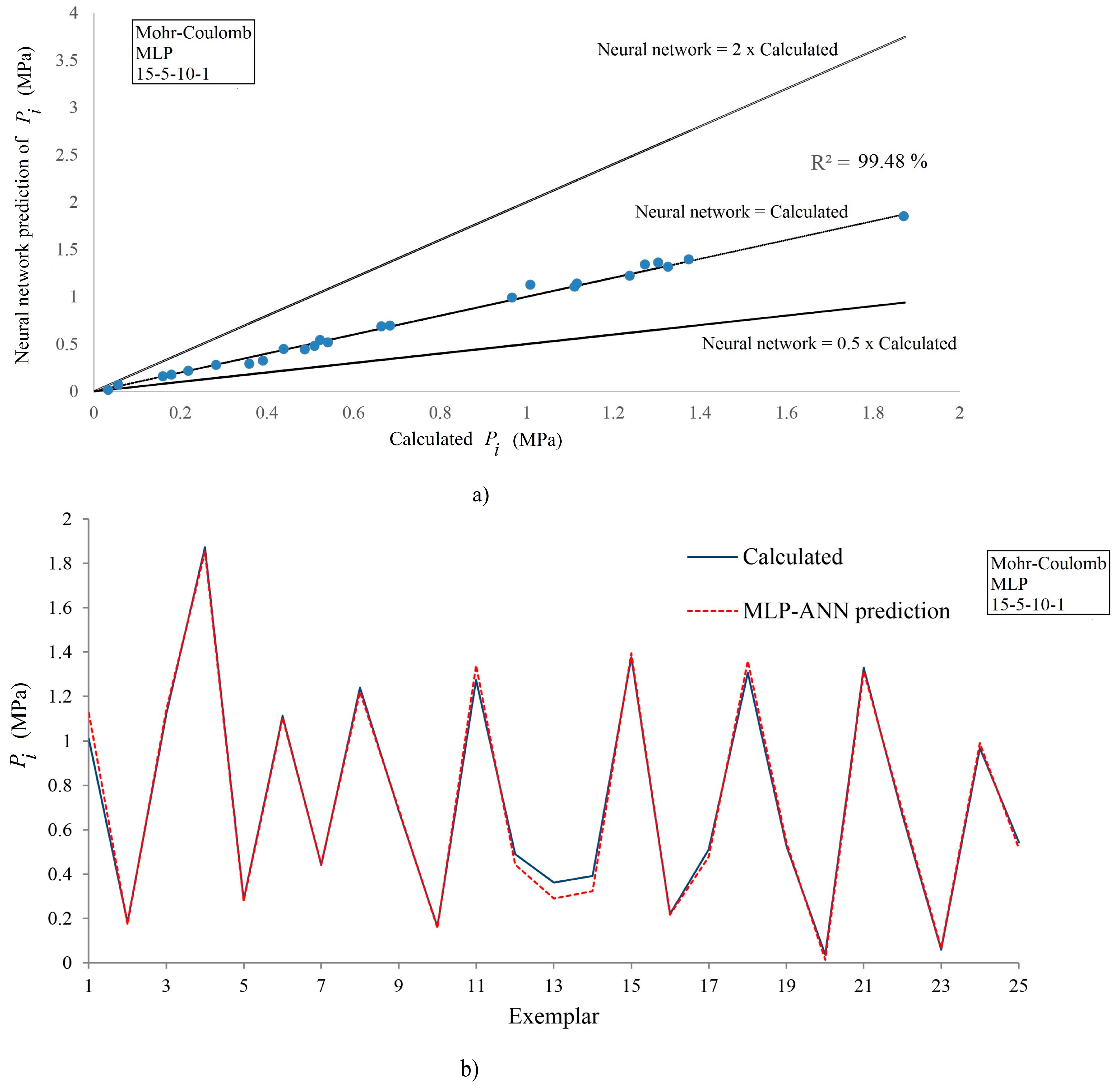
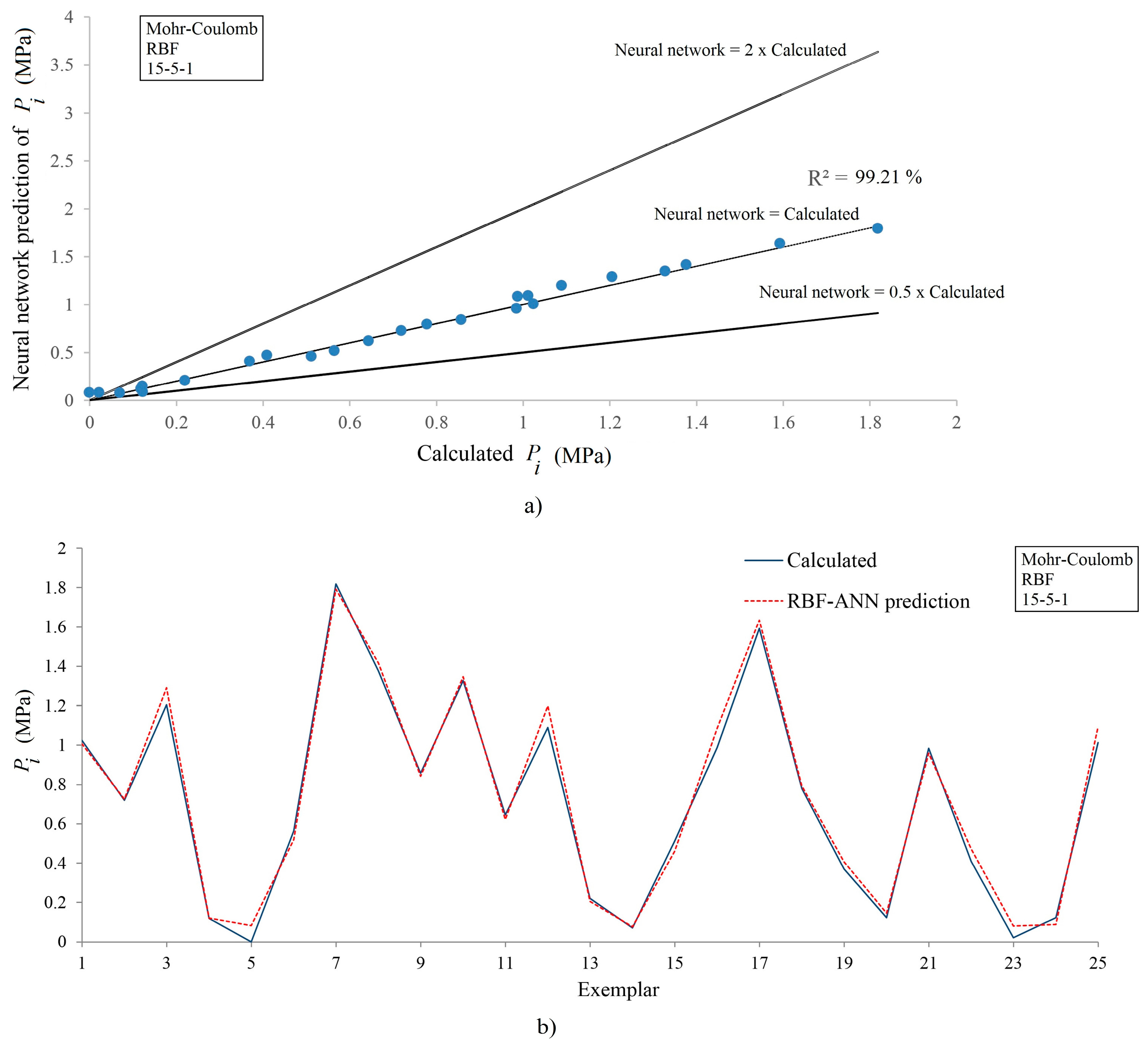
3.1. The Mohr–Coulomb Criterion
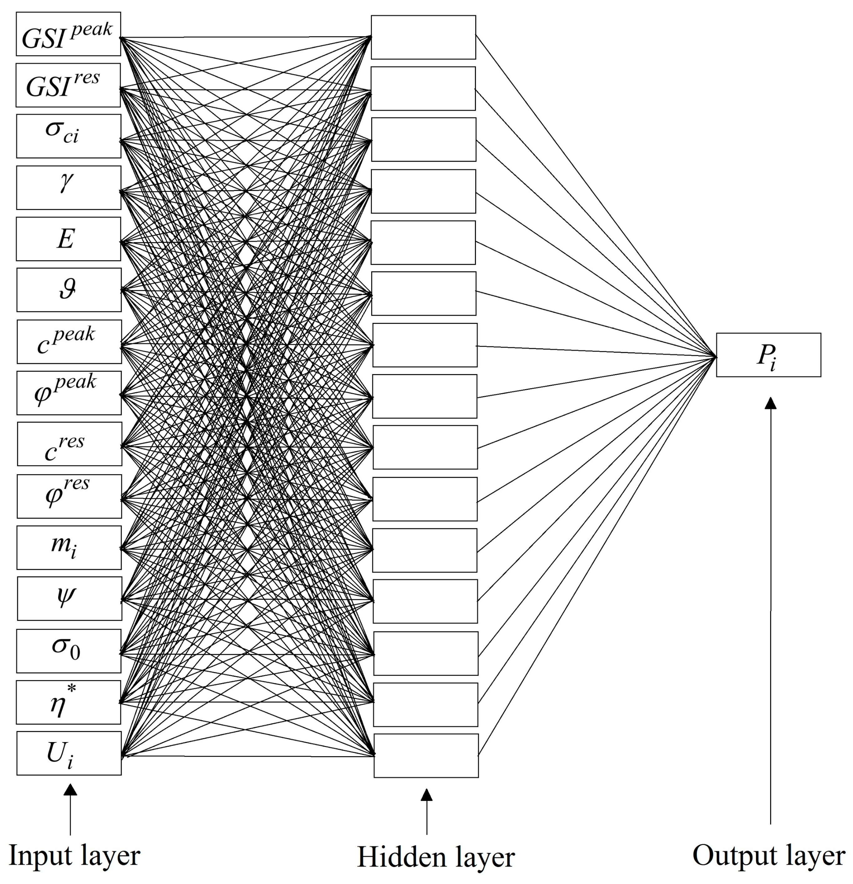
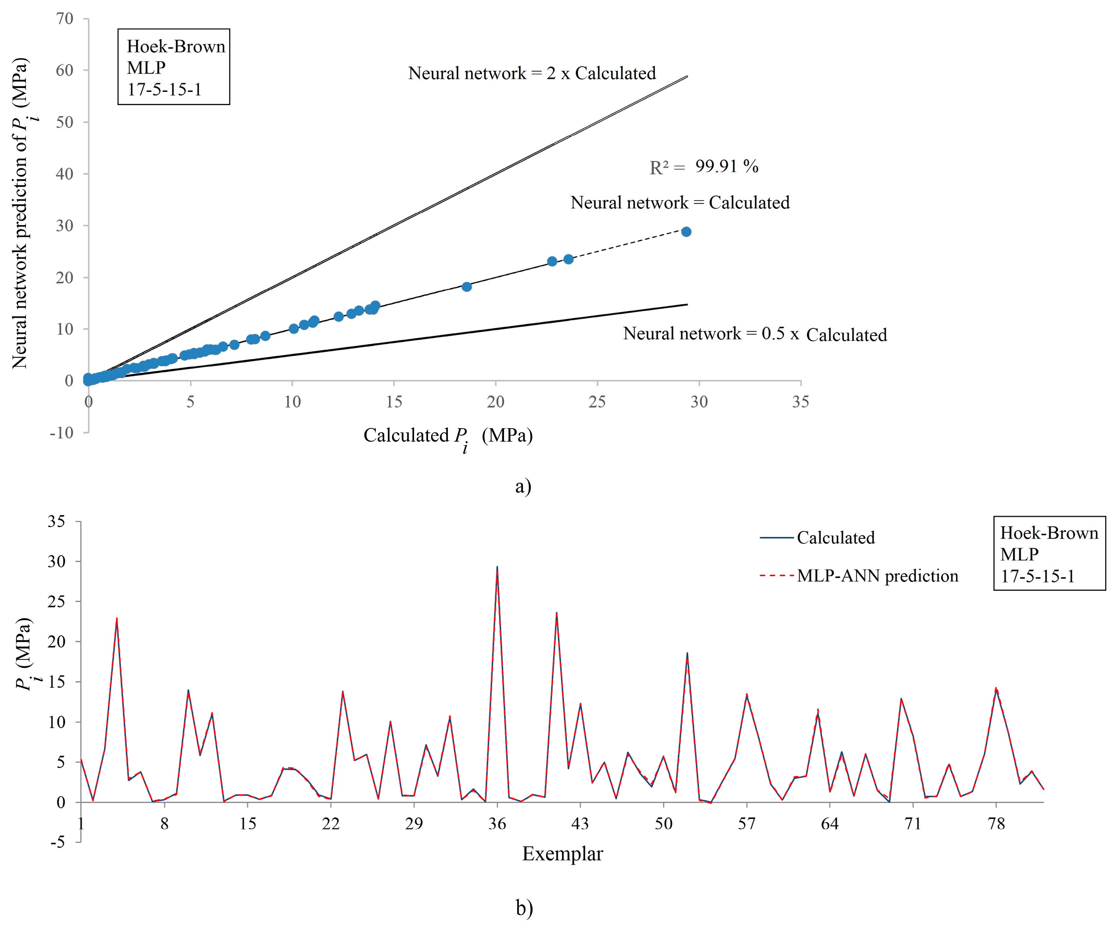
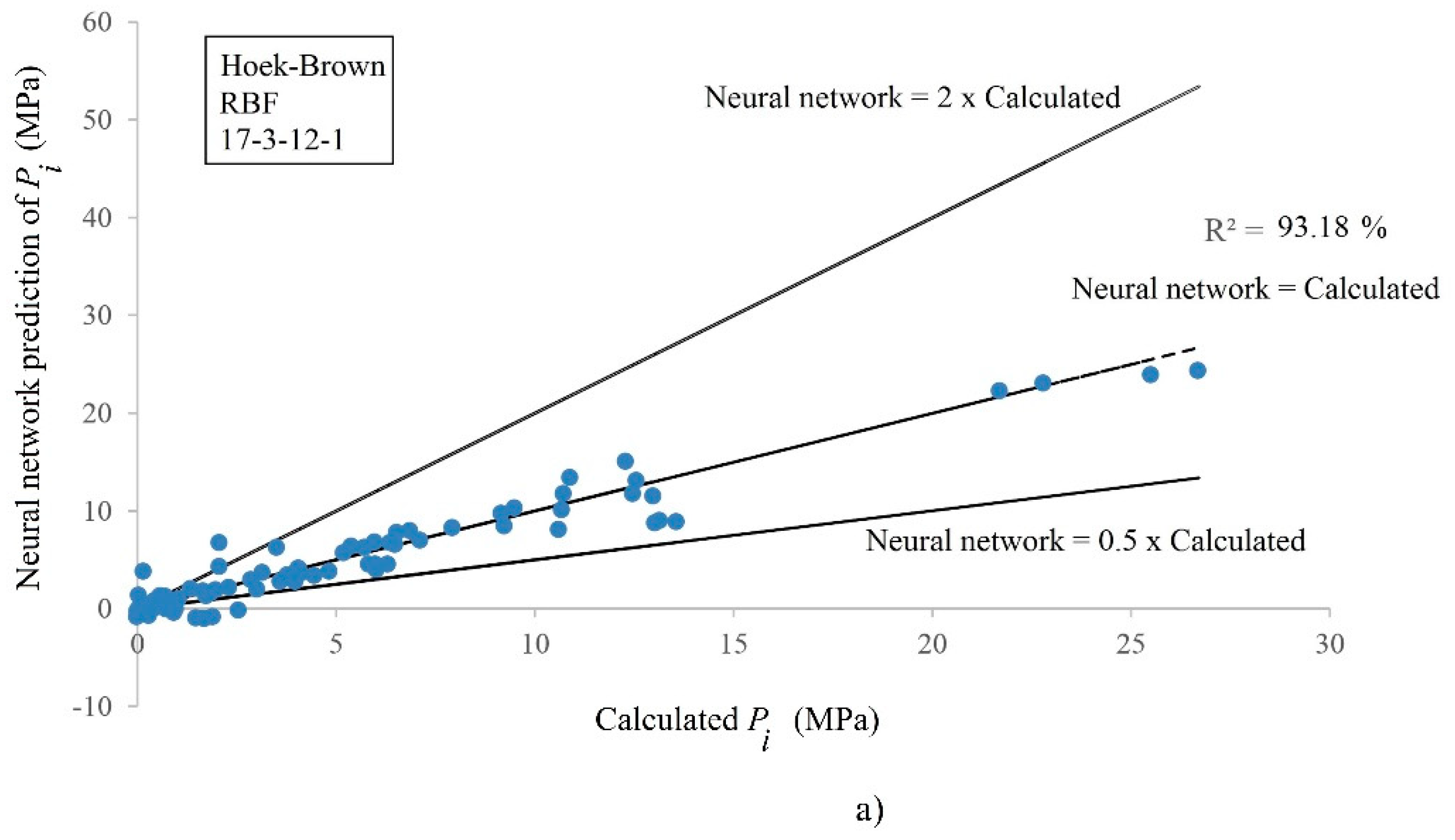
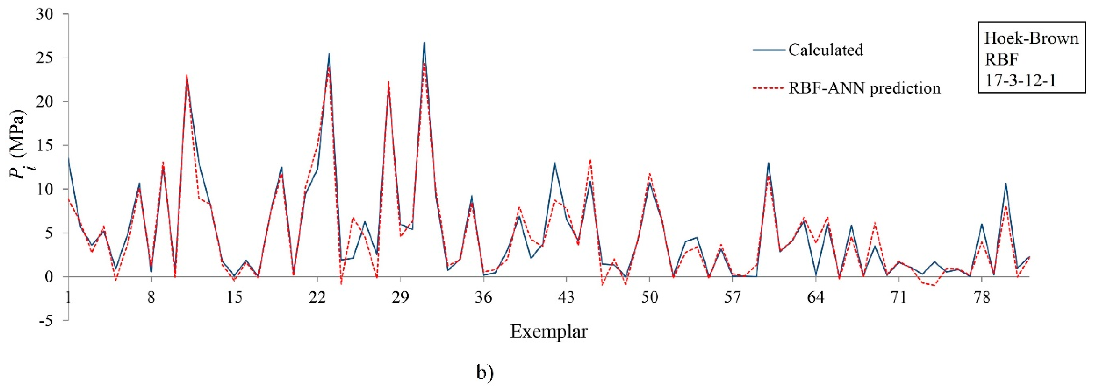
3.2. The Hoek–Brown Criterion
3.3. Comparison with Previously Obtained Models
4. Conclusions and Perspectives
- The ANN-based method appeared to be a highly performant method, applicable to the the development of GRC and the estimation of the Pi of circular tunnels;
- The 15-5-10-1 (, , and ) and 15-15-1 (, , and MPa) networks were reported as the best MLP and RBF networks for the Mohr–Coulomb case, respectively;
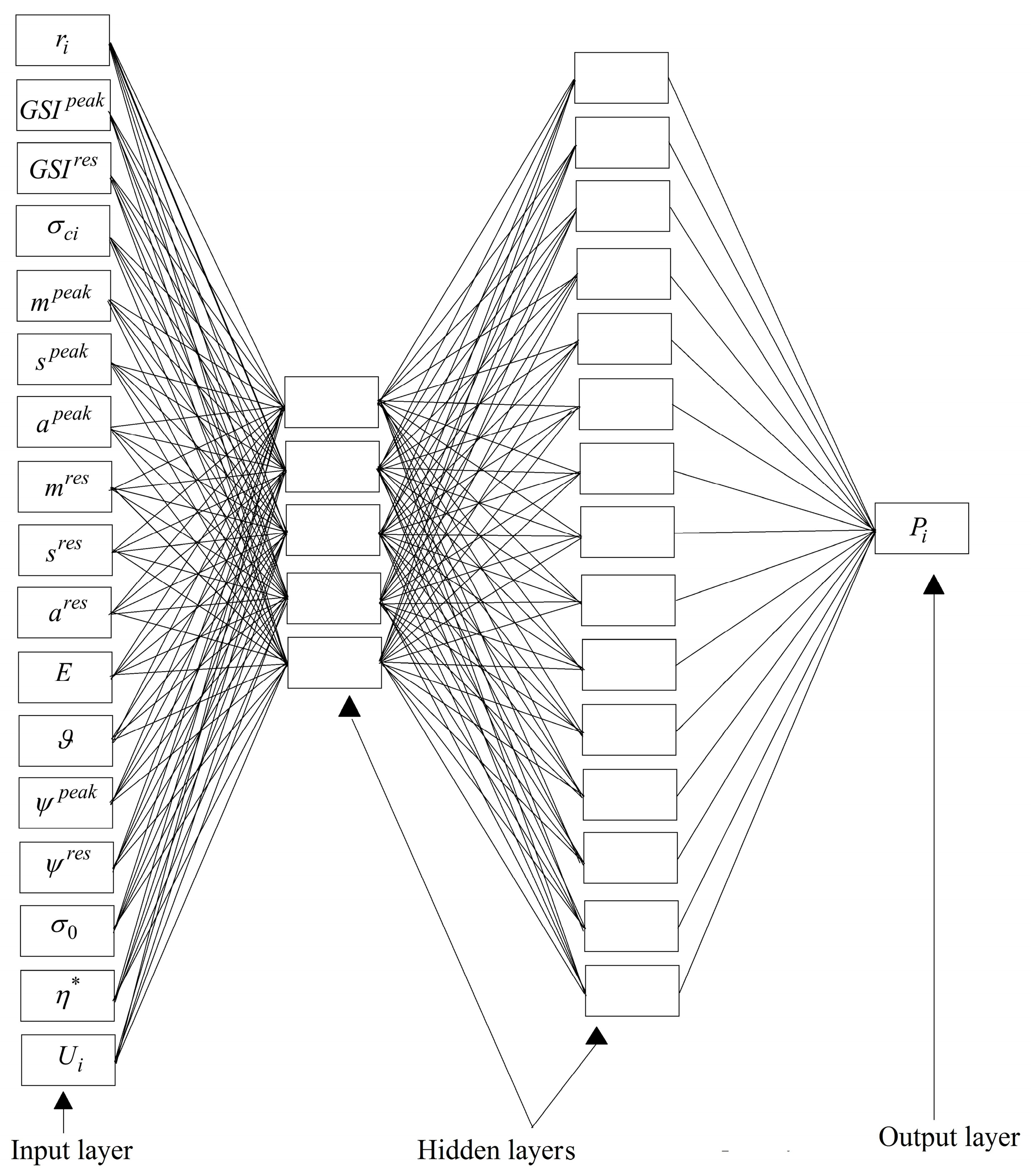
- For the Hoek–Brown case, the 17-5-15-1 MLP (, , and ) and the 17-3-12-1 RBF (, , and ) architectures were the most accurate proposed neural networks;
- It was shown that the overall performance of MLP networks was better than that of the RBF networks for both Mohr–Coulomb and Hoek–Brown cases;
- The results obtained from the comparison between neural network and EPR models proved the superiority of ANN to the EPR in the prediction of Pi;
- The proposed networks can be effectively applied by design engineers and practitioners to accurately, time-effectively, and economically obtain the GRC using a new set of data is available;
- The proposed networks can be successfully applied in conjunction with the support characteristic curve to calculate the proper time of the installation of the tunnels’ supports;
- Regarding the successful application of ANNs to the problem and as suggestion for future works, the applicability of other soft computing techniques (e.g., genetic programming, ant or bee colony, etc.) can be investigated;
- As another perspective of the current research, stress–strain and time-dependent behavior of rock masses can be studied on the basis of the implementation of viscose constitutive models;
- The formation of damaged zones around the tunnel’s surface (which is the subject of new work by the authors) and new EPR and ANN methods for the prediction of pressures are other interesting perspectives suggested by the present paper.
Author Contributions
Conflicts of Interest
Nomenclature
| Symbol | Description | Unit | Symbol | Description | Unit |
| Residual a constant | [-] | Weight between neurons | [-] | ||
| Peak a constant | [-] | Input | [-] | ||
| Calculated value | [-] | Gaussian basis function | [-] | ||
| Peak cohesion | MPa | Unit weight | kN/m3 | ||
| Residual cohesion | MPa | Softening parameter | [-] | ||
| Weighted sum of the inputs | [-] | Critical softening parameter | [-] | ||
| Young’s modulus | GPa | Poisson’s ratio | [-] | ||
| Peak geological strength index | [-] | Center of the Gaussian basis function | [-] | ||
| Residual geological strength index | [-] | In-situ stress | MPa | ||
| Mean absolute error | [-] | Uni-axial compressive strength | MPa | ||
| mi constant | [-] | Spread of the Gaussian basis function | [-] | ||
| Peak m constant | [-] | Radial stress | MPa | ||
| Residual m constant | [-] | Tangential stress | MPa | ||
| Number of datasets | [-] | Peak friction angle | ° | ||
| Predicted value | [-] | Residual friction angle | ° | ||
| Support pressure | MPa | Dilation angle | ° | ||
| Distance from the tunnel center | m | Peak dilation angle | ° | ||
| Coefficient of determination | [-] | Residual dilation angle | ° | ||
| Root-mean-square error | [-] | Peak strength parameters | [-] | ||
| Peak s constant | [-] | Residual strength parameters | [-] | ||
| Residual s constant | [-] | Radial displacement | m & mm | ||
| Tangent hyperbolic function | [-] |
References
- Brown, E.; Bray, J.; Ladanyi, B.; Hoek, E. Ground response curves for rock tunnels. J. Geotech. Eng. 1983, 109, 15–39. [Google Scholar] [CrossRef]
- Carranza-Torres, C.; Fairhurst, C. The elasto-plastic response of underground excavations in rock masses that satisfy the Hoek-Brown failure criterion. Int. J. Rock Mech. Min. Sci. 1999, 36, 777–809. [Google Scholar] [CrossRef]
- Carranza-Torres, C.; Fairhurst, C. Application of the convergence-confinement method of tunnel design to rock masses that satisfy the Hoek-Brown failure criterion. Tunn. Undergr. Space Technol. 2000, 15, 187–213. [Google Scholar] [CrossRef]
- Ghorbani, A.; Hasanzadehshooiili, H. A novel solution for ground reaction curve of tunnels in elastoplastic strain softening rock masses. J. Civ. Eng. Manag. 2017, 23, 773–786. [Google Scholar] [CrossRef]
- Lee, Y.; Pietruszczak, S. A new numerical procedure for elasto-plastic analysis of a circular opening excavated in a strain-softening rock mass. Tunn. Undergr. Space Technol. 2008, 23, 588–599. [Google Scholar] [CrossRef]
- Park, K.; Tontavanich, B.; Lee, J. A simple procedure for ground response of circular tunnel in elastic-strain softening rock masses. Tunn. Undergr. Space Technol. 2008, 23, 151–159. [Google Scholar] [CrossRef]
- Alonso, E.; Alejano, L.R.; Varas, F.; Fdez-Manin, G.; Carranza-Torres, C. Ground response curves for rock masses exhibiting strain-softening behavior. Int. J. Numer. Anal. Methods Geomech. 2003, 27, 1153–1185. [Google Scholar] [CrossRef]
- Alejano, L.R.; Rodriguez-Dono, A.; Alonso, E.; Fdez-Manin, G. Ground reaction curves for tunnels excavated in different quality rock masses showing several types of post-failure behavior. Tunn. Undergr. Space Technol. 2009, 24, 689–705. [Google Scholar] [CrossRef]
- Alejano, L.R.; Alonso, E.; Rodriguez-Dono, A.; Fdez-Manin, G. Application of the convergence-confinement method to tunnels in rock masses exhibiting Hoek-Brown strain-softening behavior. Int. J. Rock Mech. Min. Sci. 2010, 47, 150–160. [Google Scholar] [CrossRef]
- Zareifard, M.; Fahimifar, A. Analytical solutions for the stresses and deformations of deep tunnels in an elastic-brittle-plastic rock mass considering the damaged zone. Tunn. Undergr. Space Technol. 2016, 58, 186–196. [Google Scholar] [CrossRef]
- Zou, J.-F.; Li, C.; Wang, F. A new procedure for ground response curve (GRC) in strain-softening surrounding rock. Comput. Geotech. 2017, 89, 81–91. [Google Scholar] [CrossRef]
- Ghorbani, A.; Hasanzadehshooiili, H. A comprehensive solution for calculation of ground reaction curve of circular tunnels in elastic-plastic-EDZ rock mass considering strain softening. Tunn. Undergr. Space Technol. 2018. under revision. [Google Scholar]
- Ketabian, E.; Molladavoodi, H. Practical ground response curve considering post-peak rock mass behavior. Eur. J. Environ. Civ. Eng. 2017, 21, 1–23. [Google Scholar] [CrossRef]
- Hoek, E.; Brown, E.T. Practical estimates of rock mass strength. Int. J. Rock Mech. Min. Sci. 1997, 34, 1165–1186. [Google Scholar] [CrossRef]
- Santos, V.; da Silva, P.F.; Brito, M.G. Estimating RMR Values for Underground Excavations in a Rock Mass. Minerals 2018, 8, 78. [Google Scholar] [CrossRef]
- Sharan, S. Analytical solutions for stress & displacements around a circular opening in a generalized Hoek-Brown rock. Int. J. Rock Mech. Min. Sci. 2008, 45, 78–85. [Google Scholar]
- Wang, S.; Yin, X.; Tang, H.; Ge, X. A new approach for analyzing circular tunnel in strain-softening rock masses. Int. J. Rock Mech. Min. Sci. 2010, 47, 170–178. [Google Scholar] [CrossRef]
- Gonzalez-Cao, J.; Varas, F.; Bastante, F.; Alejano, L. Ground reaction curves for circular excavations in non-homogeneous, axisymmetric strain-softening rock masses. J. Rock Mech. Geotech. Eng. 2013, 5, 431–442. [Google Scholar] [CrossRef]
- Zareifard, M.; Fahimifar, A. Elastic-brittle-plastic analysis of circular deep underwater cavities in a Mohr-Coulomb rock mass considering seepage forces. Int. J. Geomech. 2015, 15. [Google Scholar] [CrossRef]
- Park, K. Large strain similarity solution for a spherical or circular opening excavated in elastic-perfectly plastic media. Int. J. Numer. Anal. Methods Geomech. 2015, 39, 724–737. [Google Scholar] [CrossRef]
- Pinheiro, M.; Emery, X.; Miranda, T.; Lamas, L.; Espada, M. Modelling Geotechnical Heterogeneities Using Geostatistical Simulation and Finite Differences Analysis. Minerals 2018, 8, 52. [Google Scholar] [CrossRef]
- Baziar, M.H.; Ghorbani, A. Evaluation of lateral spreading using artificial neural networks. Soil Dyn. Earthq. Eng. 2005, 25, 1–9. [Google Scholar] [CrossRef]
- Ghorbani, A.; Jafarian, Y.; Maghsoudi, M.S. Estimating shear wave velocity of soil deposits using polynomial neural networks: Application to liquefaction. Comput. Geosci. 2012, 44, 86–94. [Google Scholar] [CrossRef]
- Hasanzadehshooiili, H.; Lakirouhani, A.; Medzvieckas, J. Superiority of artificial neural networks over statistical methods in prediction of the optimal length of rock bolts. J. Civ. Eng. Manag. 2012, 18, 655–661. [Google Scholar] [CrossRef]
- Sadowski, Ł. Non-destructive evaluation of the pull-off adhesion of concrete floor layers using RBF neural network. J. Civ. Eng. Manag. 2013, 19, 550–560. [Google Scholar] [CrossRef]
- Sadowski, Ł. Non-destructive investigation of corrosion current density in steel reinforced concrete by artificial neural networks. Arch. Civ. Mech. Eng. 2013, 13, 104–111. [Google Scholar] [CrossRef]
- Hasanzadehshooiili, H.; Mahinroosta, R.; Lakirouhani, A.; Oshtaghi, V. Using artificial neural network (ANN) in prediction of collapse settlements of sandy gravels. Arabian J. Geosci. 2014, 7, 2303–2314. [Google Scholar] [CrossRef]
- Sadowski, Ł.; Hoła, J. ANN modeling of pull-off adhesion of concrete layers. Adv. Eng. Softw. 2015, 89, 17–27. [Google Scholar] [CrossRef]
- Ghorbani, A.; Hasanzadehshooiili, H. Prediction of UCS and CBR of microsilica-lime stabilized sulfate silty sand using ANN and EPR models; application to the deep soil mixing. Soils Found. 2018, 58, 34–49. [Google Scholar] [CrossRef]
- Asteris, P.G.; Roussis, P.C.; Douvika, M.G. Feed-Forward Neural Network Prediction of the Mechanical Properties of Sandcrete Materials. Sensors 2017, 17, 1344. [Google Scholar] [CrossRef] [PubMed]
- Asteris, P.G.; Plevris, V. Anisotropic masonry failure criterion using artificial neural networks. Neural Comput. Appl. 2017, 28, 2207–2229. [Google Scholar] [CrossRef]
- Asteris, P.G.; Nozhati, S.; Nikoo, M.; Cavaleri, L.; Nikoo, M. Krill herd algorithm-based neural network in structural seismic reliability evaluation. Mech. Adv. Mater. Struct. 2018, 1–8. [Google Scholar] [CrossRef]
- Asteris, P.G.; Kolovos, K.G.; Douvika, M.G.; Roinos, K. Prediction of self-compacting concrete strength using artificial neural networks. Eur. J. Environ. Civ. Eng. 2016, 20, s102–s122. [Google Scholar] [CrossRef]
- Asteris, P.G.; Kolovos, K.G. Self-compacting concrete strength prediction using surrogate models. Neural Comput. Appl. 2017, 1–16. [Google Scholar] [CrossRef]
- Funahashi, K.I. On the approximate realization of continuous mappings by neural networks. Neural Netw. 1989, 2, 183–192. [Google Scholar] [CrossRef]
- Zareifard, M.; Fahimifar, A. A new solution for shallow and deep tunnels by considering the gravitional loads. Acta Geotech. Slov. 2012, 2, 37–49. [Google Scholar]
- Cai, M.; Kaiser, P.K.; Tasakab, Y.; Minamic, M. Determination of residual strength parameters of jointed rock masses using the GSI system. Int. J. Rock Mech. Min. Sci. 2007, 44, 247–265. [Google Scholar] [CrossRef]
- Yasrebi, S.S.H.; Emami, M. Application of Artificial Neural Networks (ANNs) in prediction and interpretation of pressuremeter test results. In Proceedings of the 12th International Conference of International Association for Computer Methods and Advances in Geomechanics (IACMAG), Goa, India, 1–6 October 2008. [Google Scholar]
- Demuth, H.; Beal, M.; Hagan, M. Neural Network Toolbox 5 User’s Guide; The Math Work, Inc.: Natick, MA, USA, 1996; 852p. [Google Scholar]
- Girosi, F.; Poggio, T. Networks and the best approximation property. Biol. Cybern. 1990, 6, 169–176. [Google Scholar] [CrossRef]
- Tawadrous, A.S.; Katsabanis, P.D. Prediction of surface crown pillar stability using artificial neural networks. Int. J. Numer. Anal. Methods Geomech. 2007, 31, 917–931. [Google Scholar] [CrossRef]
- Heshmati, A.A.; Alavi, A.H.; Keramati, M.; Gandomi, A.H. A Radial Basis Function Neural Network Approach for Compressive Strength Prediction of Stabilized Soil. In Proceedings of the GeoHunan International Conference, Changsha, China, 3–6 August 2009. [Google Scholar]
- Lashgari, A.; Fouladgar, M.M.; Yazdani-Chamzini, A.; Skibniewski, M.J. Using an integrated model for shaft sinking method selection. J. Civ. Eng. Manag. 2011, 17, 569–580. [Google Scholar] [CrossRef]
- Sayadi, A.R.; Lashgari, A.; Paraszczak, J.J. Hard-rock LHD cost estimation using single and multiple regressions based on principal component analysis. Tunn. Undergr. Space Technol. 2012, 27, 133–141. [Google Scholar] [CrossRef]
- Plevris, V.; Asteris, P.G. Modeling of masonry failure surface under biaxial compressive stress using Neural Networks. Constr. Build. Mater. 2014, 55, 447–461. [Google Scholar] [CrossRef]
- Rafiei, M.H.; Khushefati, W.H.; Demirboga, R.; Adeli, H. Neural Network, Machine Learning, and Evolutionary Approaches for Concrete Material Characterization. ACI Mater. J. 2016, 113, 781–789. [Google Scholar] [CrossRef]
- Golafshani, E.M.; Behnood, A. Application of soft computing methods for predicting the elastic modulus of recycled aggregate concrete. J. Clean. Prod. 2018, 176, 1163–1176. [Google Scholar] [CrossRef]


| Parameter | Range of Variation | Standard Deviation | Coefficient of Variation (%) |
|---|---|---|---|
| 21.4–64.9 | 17.48 | 34.45 | |
| 15.1–33 | 6.91 | 26.20 | |
| 23–162 | 60.09 | 60.49 | |
| 26–26.7 | 0.33 | 1.27 | |
| 1.1–24 | 10.57 | 92.47 | |
| 0.25–0.3 | 0.02 | 8.27 | |
| 0.34–3.7 | 1.55 | 83.51 | |
| 24.81–57.8 | 14.26 | 33.24 | |
| 0.27–0.96 | 0.31 | 51.67 | |
| 15.69–51 | 15.42 | 42.51 | |
| 10–20 | 4.47 | 27.61 | |
| 0–14 | 6.14 | 90.30 | |
| 10.4–26 | 7.27 | 41.89 | |
| 0.0465–0.1394 | 0.037 | 43.43 | |
| 8.86–1263.69 | 307.86 | 147.24 | |
| 0–2 | 0.55 | 71.55 |
| Parameter | Range of Variation | Standard Deviation | Coefficient of Variation (%) |
|---|---|---|---|
| 3–5.35 | 0.95 | 26.78 | |
| 25–100 | 29.52 | 41.34 | |
| 10–100 | 35.89 | 67.07 | |
| 27.6–75 | 22.83 | 42.59 | |
| 1.38–36.51 | 9.03 | 112.80 | |
| 0.25 | 0 | 0 | |
| 0.5–4.09 | 0.94 | 57.06 | |
| 0.0002–0.0622 | 0.016 | 203.39 | |
| 0.5 | 0 | 0 | |
| 0.1–1.173 | 0.29 | 41.75 | |
| 0–0.002 | 0.00077 | 107.25 | |
| 0.5–0.6 | 0.03 | 5.99 | |
| 0–30 | 9.38 | 84.71 | |
| 0–20 | 5.50 | 94.45 | |
| 3.31–30 | 6.54 | 43.53 | |
| 0.004742–100 | 34.66 | 216.12 | |
| 0–0.282765 | 0.045 | 150.29 | |
| 0–29.4 | 5.63 | 107.80 |
| Architecture | ANN Type | |||||
|---|---|---|---|---|---|---|
| MLP-ANN | RBF-ANN | |||||
| R2 (%) | RMSE (MPa) | MAE (MPa) | R2 (%) | RMSE (MPa) | MAE (MPa) | |
| 15-3-12-1 | 94.47 | 0.126617 | 0.09375 | 79.42 | 0.22383 | 0.1494 |
| 15-3-15-1 | 93.61 | 0.136705 | 0.100808 | 96.51 | 0.09361 | 0.06803 |
| 15-5-1 | 92.17 | 0.163929 | 0.102924 | 65.12 | 0.346439 | 0.256144 |
| 15-5-10-1 | 99.48 | 0.03883 | 0.02825 | 77.20 | 0.3193 | 0.2607 |
| 15-5-15-1 | 91.98 | 0.185252 | 0.128403 | 69.26 | 0.320201 | 0.180665 |
| 15-10-1 | 92.31 | 0.153122 | 0.110948 | 88.89 | 0.177232 | 0.142425 |
| 15-10-5-1 | 98.63 | 0.066325 | 0.042416 | 93.37 | 0.17276 | 0.124671 |
| 15-12-3-1 | 95.99 | 0.118647 | 0.06867 | 63.24 | 0.427169 | 0.340091 |
| 15-15-1 | 98.22 | 0.075068 | 0.058276 | 99.21 | 0.050576 | 0.040918 |
| 15-15-3-1 | 93.72 | 0.164167 | 0.107004 | 87.43 | 0.182931 | 0.140225 |
| 15-15-5-1 | 99.41 | 0.0459213 | 0.028215 | 81.90 | 0.255812 | 0.190918 |
| Architecture | ANN Type | |||||
|---|---|---|---|---|---|---|
| MLP-ANN | RBF-ANN | |||||
| R2 (%) | RMSE (MPa) | MAE (MPa) | R2 (%) | RMSE (MPa) | MAE (MPa) | |
| 17-3-12-1 | 99.72 | 0.268343 | 0.204655 | 93.18 | 1.558064 | 1.078099 |
| 17-3-15-1 | 93.37 | 1.36379 | 0.965679 | 84.51 | 2.515467 | 1.703367 |
| 17-5-1 | 99.63 | 0.317273 | 0.233694 | 78.35 | 2.570293 | 1.65224 |
| 17-5-10-1 | 90.37 | 1.565927 | 1.24049 | 89.05 | 2.165716 | 1.561432 |
| 17-5-15-1 | 99.91 | 0.179285 | 0.12516 | 87.72 | 1.810275 | 1.213031 |
| 17-10-1 | 99.67 | 0.300537 | 0.225826 | 77.64 | 2.497819 | 1.639146 |
| 17-10-5-1 | 99.87 | 0.252432 | 0.164251 | 80.62 | 2.627902 | 1.729953 |
| 17-12-3-1 | 99.80 | 0.239714 | 0.167833 | 88.72 | 2.06676 | 1.310764 |
| 17-15-1 | 99.65 | 0.322873 | 0.233356 | 90.51 | 1.877567 | 1.26464 |
| 17-15-3-1 | 99.85 | 0.20853 | 0.125573 | 77.22 | 3.019557 | 2.056784 |
| 17-15-5-1 | 99.72 | 0.307093 | 0.162638 | 72.15 | 3.060725 | 2.036629 |
© 2018 by the authors. Licensee MDPI, Basel, Switzerland. This article is an open access article distributed under the terms and conditions of the Creative Commons Attribution (CC BY) license (http://creativecommons.org/licenses/by/4.0/).
Share and Cite
Ghorbani, A.; Hasanzadehshooiili, H.; Sadowski, Ł. Neural Prediction of Tunnels’ Support Pressure in Elasto-Plastic, Strain-Softening Rock Mass. Appl. Sci. 2018, 8, 841. https://doi.org/10.3390/app8050841
Ghorbani A, Hasanzadehshooiili H, Sadowski Ł. Neural Prediction of Tunnels’ Support Pressure in Elasto-Plastic, Strain-Softening Rock Mass. Applied Sciences. 2018; 8(5):841. https://doi.org/10.3390/app8050841
Chicago/Turabian StyleGhorbani, Ali, Hadi Hasanzadehshooiili, and Łukasz Sadowski. 2018. "Neural Prediction of Tunnels’ Support Pressure in Elasto-Plastic, Strain-Softening Rock Mass" Applied Sciences 8, no. 5: 841. https://doi.org/10.3390/app8050841
APA StyleGhorbani, A., Hasanzadehshooiili, H., & Sadowski, Ł. (2018). Neural Prediction of Tunnels’ Support Pressure in Elasto-Plastic, Strain-Softening Rock Mass. Applied Sciences, 8(5), 841. https://doi.org/10.3390/app8050841