Article

An Efficient Multiscale Scheme Using Local Zernike Moments for Face Recognition

1
Department of Computer Engineering, Istanbul Technical University, 34469 Istanbul, Turkey
2
Department of Computer Engineering, MEF University, 34396 Istanbul, Turkey
*
Author to whom correspondence should be addressed.
Appl. Sci. 2018, 8(5), 827; https://doi.org/10.3390/app8050827
Submission received: 3 April 2018 / Revised: 13 May 2018 / Accepted: 17 May 2018 / Published: 21 May 2018
(This article belongs to the Special Issue Advanced Intelligent Imaging Technology)

Abstract

:
In this study, we propose a face recognition scheme using local Zernike moments (LZM), which can be used for both identification and verification. In this scheme, local patches around the landmarks are extracted from the complex components obtained by LZM transformation. Then, phase magnitude histograms are constructed within these patches to create descriptors for face images. An image pyramid is utilized to extract features at multiple scales, and the descriptors are constructed for each image in this pyramid. We used three different public datasets to examine the performance of the proposed method:Face Recognition Technology (FERET), Labeled Faces in the Wild (LFW), and Surveillance Cameras Face (SCface). The results revealed that the proposed method is robust against variations such as illumination, facial expression, and pose. Aside from this, it can be used for low-resolution face images acquired in uncontrolled environments or in the infrared spectrum. Experimental results show that our method outperforms state-of-the-art methods on FERET and SCface datasets.

1. Introduction

Face recognition is actively used in many applications, such as entertainment, social media, security, and law enforcement. Despite the great deal of progress in the last two decades, face recognition systems have not fully met expectations [1]. In particular, for real-world security-related problems, powerful systems are needed that can work on images with different quality and resolutions recorded in different spectra and obtained from controlled and uncontrolled environments.
In previous studies, the face recognition problem has been tackled in different ways according to the type of data used. Among them, the number of studies on 2D still images in the visible spectrum is quite high [2]. The main reason for this is the need for methods that can be used on 2D still images for many real-world problems. On the other hand, since video recording is now performed in many environments with surveillance cameras, methods developed for use on 2D video data also have an important place in the field of face recognition [3]. In addition to illuminated environments, to also enable recognition in dark environments, heterogeneous methods are developed to compare the images in infrared and visible spectra [4]. Another example of heterogeneous face recognition is sketch-photo matching [4], which is often used to detect suspects in forensic cases. In addition to 2D data, with the easy access to sensors used to acquire 3D data in recent years, 3D face images have become widely used for facial recognition [5] and facial analysis [6] for different purposes. In this work, we propose a face recognition scheme for 2D still images in visible and infrared spectra.
The face recognition problem is generally addressed in two different ways; identification and verification. In the identification problem, the aim is to find the identity of a person from a face image. In the verification problem, it is desired to verify if two (or more) different facial images belong to the same person. The face recognition systems for both problems have two important parts: extraction of face descriptors and classification of these descriptors. The performance of these systems depends largely on the quality of the descriptors used. Therefore, there are many studies in the literature about how to construct descriptors that will maintain intra-class similarities and inter-class differences.
Face descriptors are generally divided into three parts: deep learning-based, learning-based, and hand-crafted descriptors. Significant achievements have been obtained with deep learning-based methods, especially in recent years [7,8,9]. Among these methods, convolutional neural networks (CNNs) are the most-studied method, and the highest face recognition performances are typically obtained with CNNs [10]. In the literature, many learning-based and hand-crafted representations have been proposed to construct descriptors from face images. Principal component analysis (PCA) [11], linear discriminant analysis (LDA) [12], and independent component analysis (ICA) [13] are well-known examples of the former group. In these methods, the descriptors are constructed by projecting the face images into a subspace. Because the construction of the descriptors using these methods is performed globally on the images, these descriptors are quite sensitive to variations in illumination and facial expression [14].
In most of the recent hand-crafted methods, descriptors are computed locally on face images. Local binary patterns (LBP) [15] is one of the best known local methods used in face recognition. Following its successful results, many other LBP-like methods with local encodings have been developed in the literature [16,17,18,19]. Tan et al. [20] use ternary codes (−1, 0 and 1) instead of binary codes. Zhang et al. [21] encode high-order local differences in different directions with local derivative patterns. Another recent study makes use of dual cross patterns [2]. In this method, the second-order pattern is encoded in four different directions (0, π / 2 , π , and 3 π / 4 ). Gabor wavelets [22] are another local method commonly used to construct local descriptors for face images. In the majority of studies, 40 complex images are obtained by applying 40 Gabor filters to face images in 8 different orientations and 5 different frequencies [14]. Apart from Gabor and LBP-like methods, histograms of oriented gradients (HOGs) [23], scale invariant feature transform (SIFT), [24], patterns of oriented edge magnitudes (POEM) [25] and local quantized patterns (LQP) [26] are also used to generate the descriptors.
In this study, the descriptors for face images are generated using Zernike moments (ZMs) [27]. In addition to face recognition, there are many other studies that use ZMs for different recognition problems—for instance, fingerprint [28], character [29], and iris [30]. Studies on face recognition can be summarized as follows: Foon et al. [31] introduced a face verification method which combines ZMs with wavelet transforms [32]. Ouanan et al. [33] use Gabor filters to extract texture features, and ZMs to compute facial shape features. In [34], a global feature descriptor is proposed using Gabor filters and ZMs. First, they generate multi-scale Gabor maps and then compute ZMs of these maps. In [35], the face images are divided into sub-regions and for each sub-region, and local and global features are calculated using LBP and ZMs, respectively. A similar approach is proposed by Singh et al. [36]. Along with the global ZMs, they use the local features obtained with SIFT keypoints. Huang et al. [37] modified the ZMs calculations and obtained the spatially-weighted ZMs to enhance the effect of distinctive regions on the face. In [38], the ZMs are calculated separately for the non-overlapping sub-regions of the face images, and the moments are weighted adaptively according to the regions.
It is known that powerful descriptors can be constructed with ZMs for images which have explicit shapes, such as fingerprint and optical characters [28,29]. However, for face recognition, local structures are more distinctive and prominent than global shape information. For this reason, as mentioned above, along with the local feature extraction operators, ZMs are used for general shape characteristics of face images in most of the previous studies. To expose local patterns from face images using ZMs in a robust way, in our previous work we developed a method called the local Zernike moments (LZM) transformation [39]. In contrast to ZMs calculated from the entire image, LZM representation is obtained by applying the ZM transform at each pixel using its neighborhood to capture the micro-structure around this pixel. By using the complex ZMs calculated for each pixel, a different number of complex images are generated according to the moment degree. Different studies have been carried out on face recognition with LZM transformation. In [40], using a scale-space representation, a face identification method for low-resolution images is proposed. Kahraman et al. [41] have developed a face verification method with metric learning techniques on the feature vectors generated from LZM maps. In some studies, complex images obtained by LZM transformation have been encoded using different operators, and then descriptors have been created for face images. Basaran et al. [42] use local Zernike xor patterns (LZXP) obtained by encoding LZM images with the xor operator. In [43], real and imaginary LZM components are encoded with a local phase quantization method. In addition to face recognition, there are also some studies on facial expression recognition using LZM transformation. Sariyanidi et al. [44] proposed quantized local ZMs encoding complex ZMs with binary quantization. In [45], LZM features are used with LZXP features and global ZMs.
A face recognition scheme developed using complex LZM components is proposed in this work, named multi-scale local Zernike moments (MS-LZM). Similar to [39], in MS-LZM, the LZM transformation is applied twice in succession. With the first transformation, the effects of lighting and blurring on the images are removed. The outputs of the second transformation are used to create feature vectors for face images. In most studies using local methods [20,46,47], the images generated by encoding with the local operators are divided into sub-regions and histograms are calculated in each sub-region to obtain the features. Recently, methods that use features around facial points have become popular [2,48,49], and we prefer to use this approach. For each complex LZM component, we calculate the phase-magnitude histograms (PMHs) on the patches around the facial points. Then, these PMHs calculated on all components are concatenated to form a feature vector for each facial point. Using both local and global shape properties improves performance [50]. Hence, we build an image pyramid and calculate the features using the images of each different scale. In this way, the local and global patterns are extracted by using large- and small-scale images, respectively. In the last step of MS-LZM, the dimension of the feature vectors obtained for each facial point is reduced using whitened principal component analysis (WPCA) [51].
In recent years, high-performance face recognition methods [7,8,9,52] have been developed using deep learning techniques. For the training of the proposed models in these supervised methods, a large number of labeled images are needed. Models that are trained in some studies are shared with the public. However, when these studies are to be repeated for any real-world problem, both data and some high-quality hardware are needed. MS-LZM proposed in this study does not require any labeled images, since it is an unsupervised method. In addition, PCA matrices can be easily learned using very few images.
In our previous work [53], we used multiple grids of different sizes to extract features around facial points from single-scale LZM components, and we showed the performance of the proposed method on images obtained from controlled environments. In this study, face images are encoded with the LZM transformation in a multi-scale manner, and the features are extracted from the resulting multi-scale LZM components using a single grid. To evaluate the method, we used three different datasets with different properties. The contributions of this study are as follows: (1) In previous studies using LZM transformation, methods have been proposed for only face identification [39,42,43,53] or verification [41]. In this study, we develop an unsupervised face recognition scheme for both identification and verification; (2) In most of the LZM-based studies [39,41,42,53], only one dataset is used to evaluate the methods. In this study, using Face Recognition Technology (FERET) [54], Labeled Faces in the Wild (LFW) [55], and Surveillance Cameras Face (SCface) [56] datasets, which have very different characteristics from each other, we show the performance of MS-LZM (the code will is available at https://github.com/ebsrn/lzm-face) on unconstrained and low-resolution images acquired in uncontrolled environments or in infrared spectrum. Therefore, this work is important to show that the LZM transformation can be used successfully in very different real-world conditions; (3) The experimental results demonstrate that the proposed approach outperformed the state-of-the-art for FERET and SCface. In addition, the results for LFW were comparable to the best known results in literature.

2. Local Zernike Moments Transformation

In this section, we first give general information about Zernike moments. We then describe the local Zernike moments transformation that allows ZMs to be computed locally around each pixel.

2.1. Zernike Moments

Zernike moments consist of Zernike orthogonal polynomials defined in polar coordinates [27]. Two-dimensional Zernike moments with moment order n and repetition m of an image f ( i , j ) , whose pixel coordinates ( x i and y j ) scaled to range of [ 1 , 1 ] using (3), are represented as follows [27]:
Z n m = 2 ( n + 1 ) π ( N 1 ) 2 i = 0 N 1 j = 0 N 1 V n m ( ρ i j , θ i j ) f ( i , j ) ,
V n m ( ρ , θ ) = R n m ( ρ ) e j m θ ,
x i = 2 i + 1 N 2 ( N 1 ) , y j = 2 j + 1 N 2 ( N 1 ) ,
where ρ i j = x i 2 + y j 2 and θ i j = t a n 1 ( y i / x i ) . In (1), V n m ( ρ , θ ) represents the Zernike polynomials which are defined in polar coordinates within a unit circle, and R n m ( ρ ) represents real-valued radial polynomials. These polynomials are defined as:
R n m ( ρ ) = k = 0 n | m | 2 ( 1 ) k ( n k ) ! k ! ( n + | m | 2 k ) ! ( ( n | m | ) 2 k ) ! ρ n 2 k .
In the above equations, n and m parameters take values as 0 n , 0 | m | n , and n | m | is even. Zernike polynomials calculated using n values up to 5 are illustrated in Figure 1.

2.2. Local Zernike Moments

Zernike moments describe the holistic characterization of images using radial polynomials at different orders and repetitions. Each of these radial polynomials used corresponds to a different characteristic of the image [57]. In problems such as face recognition, rather than the holistic characterization of images, local statistics have more importance [14]. Therefore, the local Zernike moments (LZM) [39] transformation was proposed to extract local variations by calculating these moments around each pixel on the face images.
In the LZM transformation, V n m ( ρ , θ ) are used as k × k filtering kernels:
V n m k ( i , j ) = V n m ( ρ i j , θ i j ) .
Because Zernike polynomials are defined in polar coordinates, the real and imaginary components of these filters can be obtained by converting the filters to cartesian form. The real and imaginary components of the filtering kernels calculated with n values up to 5 are shown in Figure 1. Using V n m k ( i , j ) filtering kernels in (1), the ZMs around each pixel are calculated as follows [39]:
Z n m k ( i , j ) = 2 ( n + 1 ) π ( k 1 ) 2 p , q = k 1 2 k 1 2 f ( i p , j q ) V n m k ( p , q ) .
Since the imaginary component of ZMs for m = 0 is not available, the filters calculated using m values different from 0 are used in the LZM transformation. As a result, a different number of complex images are obtained depending on the value of n used. The number of these images can be calculated using:
K ( n ) = { n ( n + 2 ) 4 if n is even , ( n + 1 ) 2 4 if n is odd .
Figure 2 shows the real and imaginary components obtained for a face image using LZM filters given in Figure 1.

3. MS-LZM Face Recognition Scheme

The steps of the proposed feature extraction scheme using LZM components are shown in Figure 3.
In this scheme, we first construct an image pyramid to extract both local and global features from face images. Then, on the images in the pyramid, we apply the LZM transformation twice in succession. As explained in Section 3.2, it is aimed to eliminate the effects of lighting and blurring on the images with the first LZM transformation. The complex components obtained with the second LZM transformation are used to compute the features. We extract these features from the regions around the facial points which are detected on the face images. By concatenating the feature vectors constructed using multi-scale LZM maps, we obtain a rich representation for each facial point. At the last stage, we use WPCA to reduce the dimensions of the vectors and also to obtain more distinctive vectors. In this section, we explain these steps in detail.

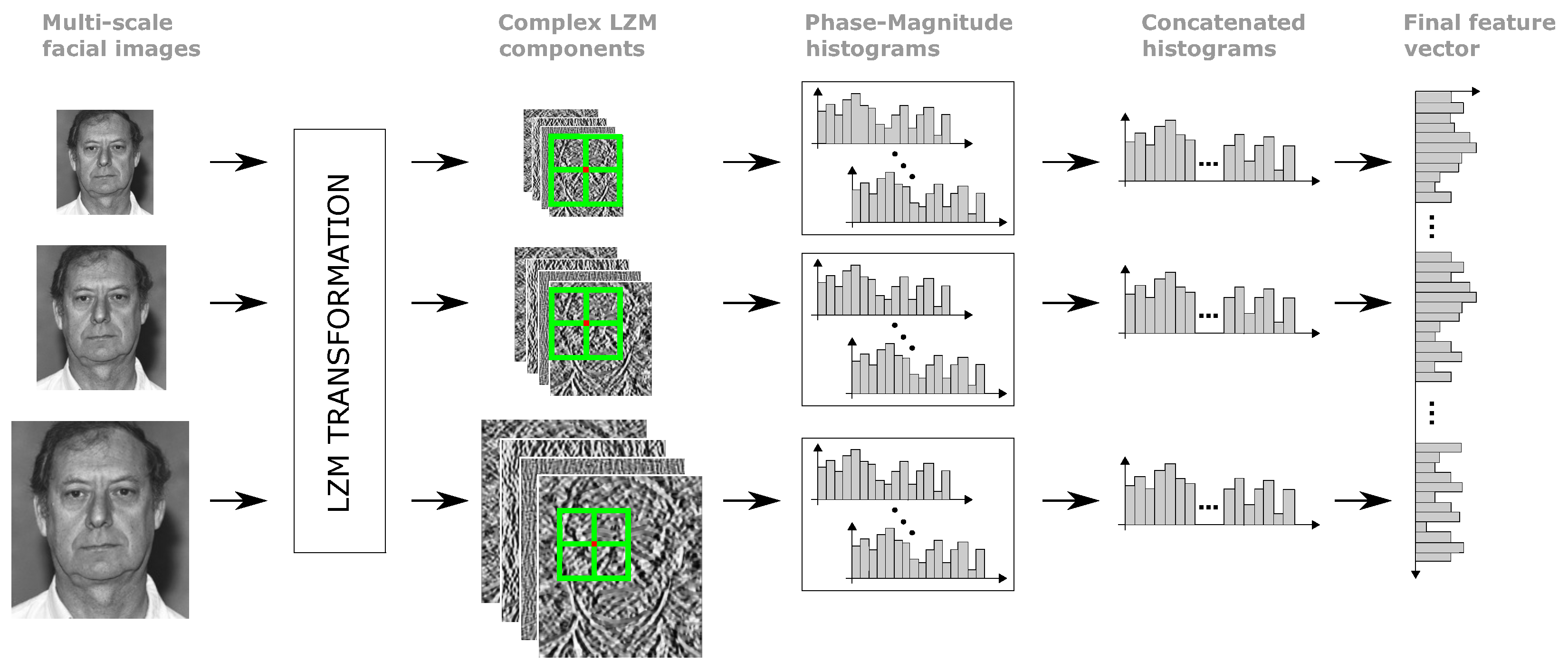
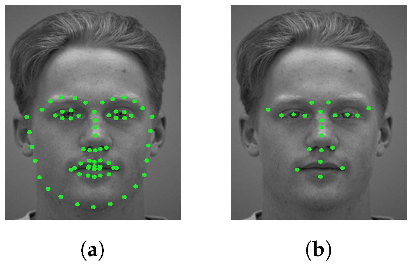
3.1. Multiscale Feature Extraction Around Facial Points

In MS-LZM, an image pyramid is created by sub-sampling the face images by a factor of 3 / 4 for each coordinate, and then the LZM transformation is applied on these images separately. On the complex-valued images obtained as a result of these transformations, the feature vectors are constructed around the points corresponding to the facial points determined on the facial image. To calculate these feature vectors, overlapping grids are located on the LZM components to be the facial points at the central point, and a phase-magnitude histogram (PMH) is constructed as described in [39] for each sub-region of these grids as follows:
P M H = [ h 0 , h 1 , h 2 , , h B 1 ] ,
where
h b = i , j A ( I i , j ) s ( Φ ( I i , j ) , b , B ) .
Here, I is a complex image, and i and j indicate pixel coordinates. A ( I i , j ) and Φ ( I i , j ) represent magnitude and phase, respectively. With real r e ( I i , j ) and imaginary i m ( I i , j ) parts of I i , j , these are computed as follows:
A ( I i , j ) = i m ( I i , j ) 2 + r e ( I i , j ) 2 ,
Φ ( I i , j ) = t a n 1 ( i m ( I i , j ) / r e ( I i , j ) ) .
In (8) and (9), B represents the number of bins in the PMH, and the function s ( ϕ , b , B ) , which is used in (9), defined as
s ( ϕ , b , B ) = 1 , if 2 π b B ϕ < 2 π ( b + 1 ) B , 0 , otherwise .
The PMHs computed for each facial point on the LZM components of different sizes are concatenated to obtain a feature vector for each facial point. To detect the facial points, we used a toolkit [58] which contains the implementation of the method proposed by Kazemi et al. [59]. In Figure 4a, the detected 68 facial points are shown. In this study, not all of these points were used. Only the 21 points given in Figure 4b were used, and to determine these points, we performed some experiments. We created subgroups using points around the eyes, mouth, and nose. Then, we selected the group with the highest performance in the experiments.

3.2. Cascaded LZM Transform

Recognition performance is directly related to the quality of the face images. Undesirable conditions such as illumination and blur on images can cause serious differences between images of the same person. To avoid this unfavorable effect on textures, it is recommended to calculate the gradient information of the images and to use this gradient information to extract the texture features [60,61]. There are many studies that have adopted this approach in face recognition. Ding et al. [2] calculated the gradient values at four different angles on the face images before performing the feature extraction with local operators. Likewise, in [46], they calculated the features with local operators using horizontal and vertical gradient values.
In this study, the LZM transformation is applied twice in succession as suggested in [39]. As a result of the first transformation, complex images are obtained from the facial image. Then, the LZM transformation is applied again on the real and imaginary components of these complex images. With the first transformation, the unfavorable features such as illumination and blur on the face images are eliminated, as it is done by calculating the gradients in the other studies mentioned above. The PMHs described in the previous section are calculated on the complex images obtained from the second transformation.

3.3. Dimensionality Reduction and Distance Calculation

By using the method described in Section 3.1, a feature vector is computed for each facial point. In this study, Whitened Principal Component Analysis (WPCA) [51], which is an unsupervised dimension reduction method, is used to both reduce the size of these feature vectors and improve face recognition performance.
In the dimension reduction process with PCA, an orthogonal projection matrix U is learned by using training data, and the dimensions of the feature vectors are reduced by using this matrix. U consists of eigenvectors corresponding to eigenvalues that are sorted from large to small. Hence, rather than the distinguishing properties, the general properties of the face images are encoded with the first vectors in the U matrix [2], and the effect of these encoded values on the face recognition performance is high [62]. In order to overcome this problem, WPCA is a widely-used method. In WPCA, each eigenvector in U is divided by the square root of its own eigenvalue, and in this way, the effect of the distinguishing properties of face images is enhanced.
In this paper, the similarity values between facial points are used to calculate the similarity between two facial images. First, the similarities between the feature vectors whose dimensions are reduced by WPCA and belong to the same facial point are calculated. Then, these similarity values are summed up, and thus the similarity between the two facial images is obtained.
There are many similarity and distance functions commonly used in literature to calculate similarity values. Since these functions have direct effects on performance [63], extensive research has been conducted to determine the most appropriate method. As a result, it is found that the best performance is obtained using weighted angle-based similarity, which is used in [46] to compute the distance between the vectors projected into WPCA subspace, given as:
s ( X , Y ) = i = 1 N z i x i y i i = 1 N x i 2 i = 1 N y i 2 , z i = 1 / λ i ,
where X and Y are the feature vectors and λ i is the eigenvalue of the ith vector of matrix U. As noted above, the features computed using the eigenvectors corresponding to the large eigenvalues are not useful for face recognition. For this reason, in (13), we reduce the contribution of features that include general information about the faces, using inversely proportional weights to the eigenvalues.

4. Experimental Results

In order to evaluate the performance of MS-LZM, we performed experiments on three different face datasets which are frequently used in the literature. The first of these was FERET [54], and using this, the identification performance of MS-LZM was evaluated. In addition to this, since there is only one image for each person in the gallery of this dataset, single sample per person success was also tested. LFW [55] was another dataset used in the experiments and is a dataset collected for the verification problem. The evaluation of the verification performance of MS-LZM was measured by performing experiments on this dataset. The last dataset used in this study was SCface [56], which has very-low-resolution probe images. This dataset was used to observe the performance of MS-LZM for video surveillance.
Some preprocessing operations were done on the images in the datasets mentioned above before the feature extraction. First, the images were aligned using a similarity transform so that the horizontal coordinates of the eyes were the same. Then, an image pyramid was generated because a multi-scale feature extraction approach was adopted in this study. The number of scales used differed according to the dataset since each image was presented in different sizes and resolutions in each dataset. While more scales and higher image sizes were used for datasets with high-resolution images, less scales and smaller image sizes were used for datasets with low-resolution images. To remove the effect of illumination on the images in the image pyramid, images were normalized to have unit variance and zero mean, and the resulting images were used in the feature extraction process. This process was performed as described in Section 3. On the aligned and normalized face images, the cascaded LZM transformation was applied and then PMHs were calculated using the complex images obtained by the second transformation. Before each LZM transformation, we separately re-normalized the k × k local regions to be encoded to have zero mean and unit variance. In order to calculate PMHs, as a result of the experiments, we decided to use 18 bins for each histogram and 40 × 40 grids with 4 × 4 cells which were located at each facial point. After normalizing PMHs using the z-score, all histograms were concatenated and thus a feature vector for each facial point was constructed. In the last stage, WPCA was applied on the feature vectors, and for each facial point, descriptors with a length of 1000 were obtained.

4.1. Experiments on FERET

FERET [54] includes a gallery set called Fa and four different probe sets called Fb, Fc, Dup1, and Dup2. There are 1196 different people in Fa, and each person has only one image. In the probe sets, there are 1195, 194, 722, and 234 images, respectively. The images in Fb have different facial expressions and the same lighting conditions as those in Fa, and these two sets are composed of images which were recorded with the same camera on the same day. Likewise, Fc and Fa sets also consist of images which were recorded on the same day. However, these images have different lighting conditions. The images in Dup1 were recorded in the same year as the images in Fa, but on different days. The last probe set Dup2 consists of images which were recorded in different years from the images in Fa. Dup1 and Dup2 sets were recorded using different cameras. These sets have facial expressions, occlusion, scale, and lighting conditions than Fa. In Figure 5, some sample images taken from FERET are shown. We followed the standard protocol of FERET in the experiments and reported the identification performance with Rank 1 recognition rate.
The characteristics of the filters used in the LZM transformation are quite different from each other, as shown in Figure 1. Therefore, different features of face images are extracted with each filter. In order to understand the effects of these filters on the recognition performance, we computed features separately with the filters obtained for each different ( n , m ) pair. Using these features, the results achieved for Fb, Fc, Dup1, and Dup2 are shown graphically in Figure 6.
When these results were calculated, facial images were used in only one scale and resized so that the distance between the eyes was 80 pixels. Feature vectors were constructed around the 21 facial points shown in Figure 4. Dimensionality reduction was not performed on the vectors and the L1-norm was chosen as the distance criterion, since we did not have eigenvalues to use the similarity function given in (13).
In the graphs given in Figure 6, the results computed using the filters up to n = 6 are shown. The blue markings on these graphs show the recognition rates achieved using each filter separately. The red markings (cumulative results) show the rates achieved using the concatenation of the feature vectors which are computed using filters up to n = 6 . When these results were examined, it was seen that the performance of each filter was quite different, especially for Dup1 and Dup2. The sixth filter corresponding to n = 4 and | m | = 4 pairs had the lowest success for Fb, Dup1, and Dup2. When cumulative results were examined, it could also be seen that the filters with low success had no negative effect on the result. The second and fifth filters were the most successful. In particular, the success achieved with the fifth filter was the same as the cumulative success.
The LZM transformation was applied twice in succession in this study. Therefore, in order to analyze the changes in performance when filters were used repeatedly, the graphs given in Figure 7 were generated for Dup1 and Dup2. Here, the results obtained with filters up to n = 4 in the first transform and up to n = 5 in the second transform are shown. In order to make a better comparison, the results given in Figure 6 are also shown in Figure 7. The best results for Dup1 and Dup2 (the cumulative filter results when n = 6 and | m | = 6 ) from Figure 6 are given by the green horizontal lines. The yellow markings show the performance per filter from Figure 6. These results are shown in accordance with the values of n 2 and | m 2 | , and they are repeated for each different n 1 and | m 1 | pair. Comparing blue and yellow markings, it can be seen that better results could be obtained for the majority of filters if the filters were applied in succession. In addition, when red markings and green lines are compared, it is clear that better results were achieved with cascaded LZM transformations. As mentioned in Section 2, LZM is a linear transformation. Therefore, the filters used in the cascaded LZM transformation can be combined, and with the filters obtained in this way, complex LZM images can be generated. In Figure 8, we compare Dup2 results calculated using the cascaded and the combined filters which are obtained using different n and | m | values. As can be seen from these results, using the cascaded and the combined filters, very close results were obtained, as expected. The reason why the results were not exactly the same is that in the cascaded LZM transformation, the local regions were normalized separately before each transformation.
In this paper, as described in Section 3, a multi-scale feature extraction method, MS-LZM, is proposed. In this method, the features are computed around the facial points and the sizes of the feature vectors obtained for each point are reduced individually using WPCA. It was mentioned earlier that 21 facial points were specified. For the number of scales and the sizes of the face images, we performed comprehensive experiments, and we decided to use the images in five different sizes as follows: 300 × 300 , 225 × 225 , 168 × 168 , 126 × 126 , a n d 94 × 94 . For 300 × 300 images, the eye coordinates were set to ( 110 , 122 ) and ( 185 , 122 ) . Aside from this, moment degrees and size of the filters used in the LZM transformations must also be determined. As a result of the experiments carried out, the best performance was achieved when the moment degree was n = 4 and the filter size was k = 5 for both LZM transformations. The results obtained are given in Table 1 together with the best known results in the literature.
While these results were calculated, the feature vectors were constructed concatenating the PMHs with 18 bins which were calculated in each 4 × 4 cells of 40 × 40 grids. The dimension of the feature vectors was reduced to 1000 with WPCA. Using Equation (13), the similarity values between the vectors, whose dimensions were reduced, corresponding to the same facial point were calculated and further summed in order to obtain the similarity between two face images.
In the results given in Table 1, it is obvious that the best identification results were obtained with the proposed method. Only four images from the Fb set could not be correctly identified. However, this is almost the same level as the highest results for this set. The results for the Fc set were all 100%. The superiority of MS-LZM is evidenced by the results obtained for Dup1 and Dup2. The images in these sets were recorded at different times from the gallery set and are the hardest sets in FERET. All studies compared in Table 1 use local feature extraction, methods as in MS-LZM. The results obtained in these studies using different local operators, including Gabor and LBP, were not better than the results obtained using LZM features in this study. On the other hand, our results are higher than those given in other studies [42,53] using LZM features. In [2,53], features are obtained around the facial points and the dimensions of the vectors are reduced with WPCA. Therefore, these methods are structurally more similar to MS-LZM. However, the results obtained in this study are better than the results achieved in both studies.

4.2. Experiments on LFW

Labeled Faces in the Wild (LFW) [55] is composed of images collected over the web. For this reason, the dataset is quite rich in terms of variations in photo quality, pose, illumination, resolution, age, race, accessories, make-up, occlusion, background, and facial expression. There are 13,233 face images detected by the Viola–Jones face detector [67], and 5749 different people in this dataset. There is a different number of images for each person, and the number of people with two or more images is 1680. Within LFW, there are two separate sets called View1 and View2. View1 was used for model selection and algorithm development, and View2 was used for calculating the success of the used methods. View2 has 10 subsets, and the images in the subsets do not overlap with each other. In each subset, there are 300 matched and 300 unmatched pairs. While performance was being calculated, 10-fold cross-validation was performed using 10 subsets. The performance for each subset was calculated separately and the remaining 9 subsets were used for training operations. In studies conducted in the literature, the results obtained are generally given in six different categories. Unsupervised methods are compared in one of them, and supervised methods are compared in the other. In this study, since an unsupervised method is used, the results obtained are given together with the best known results in the unsupervised category. In many studies in the literature, besides the original LFW, frontalized versions of this dataset are also used. In this study, we use the images which are frontalized with the method proposed by Zhu et al. [49]. Sample images (original and frontalized) of this dataset are given in Figure 9. To measure the verification performance on LFW in the unsupervised category, the area under the curve (AUC) of the receiver operating characteristic (ROC) curve was used as specified in its standard protocol [55]. The AUC value for each subset was calculated, and the average of these AUC values is reported.
Table 2 shows the results obtained using MS-LZM for LFW together with the best known results in the literature. While these results were calculated, face images were used in five different scales, and the sizes used for images were the same as those used in FERET experiments. For first and second LZM transformations applied on multi-scale images, the moment degrees were four and the filter sizes were seven. When the experiments were performed on this dataset, WPCA matrices were learned using 1200 images randomly selected from nine subsets other than the subset used for the performance calculation.
As in Table 1, in the methods compared in Table 2, the features for face images were computed using local operators. With MS-LZM, we obtained better results than the others except for MRF-Fusion-CSKDA [73]. In MRF-Fusion-CSKDA (which is proposed only for the verification problem), features were obtained with three different local methods (Multiscale Local Binary Patterns (MLBP) [74], Multiscale Local Phase Quantization (MLPQ) [75], and Multiresolution of Binarised Statistical Image Features (MBSIF) [76]), and these features were fused with a nonlinear binary classifier (CSKDA [73]). In this study, we used only LZM features and propose MS-LZM for both identification and verification problems.

4.3. Experiments on SCface

SCface [56] is a dataset that has been created in accordance with real-world conditions [56]. Images in this dataset were recorded in uncontrolled indoor environments using seven surveillance cameras with different qualities and resolutions. Two of these cameras recorded in infrared spectrum (IR). While the images were being recorded, the cameras were placed at a higher position than the heads of the people (at a height of 2.25 m) and images were taken at three different distances: 4.2 m, 2.6 m, and 1 m. There are a total of 4160 images taken from 130 different people in the dataset.
Within SCface, there are two different identification protocols, DayTime and NightTime. In the DayTime protocol, a gallery set consisting of mugshot images of 130 different people is used, and there are a total of 15 probe sets created from images taken at 3 different distances using 5 different cameras (cam1-5). In the NightTime, both the gallery images used in the DayTime protocol and a gallery set consisting of 130 mugshot images recorded in infrared spectrum can be used as a gallery set. In this protocol, there are a total of six probe sets which are created with the IR images taken at three different distances using two different IR cameras. Grgic et al. [56] recommend that external images should be used as a training set, so that the results obtained in these protocols are more consistent. Therefore, the Fa set of FERET was used to learn the PCA matrices in the experiments performed in this study. According to the standard protocol of SCface, the identification performance was given as Rank 1 recognition rate, as it was in FERET.
Sample images of SCface are presented in Figure 10. There are too many images with low resolution in this dataset. For this reason, the feature vectors, which were constructed using the images in five different scales in the previous sections, were constructed here in only three different scales. Face images were resized to three different sizes as follows: 126 × 126 , 94 × 94 , and 70 × 70 . For the 126 × 126 image, the eye coordinates were set to ( 50 , 66 ) and ( 75 , 66 ) . When facial images are used in larger sizes, identification performance is adversely affected because low-resolution images reduce between-class differences.
Table 3 shows the results obtained for the DayTime protocol with the best known results in the literature. While these results were calculated, the moment degrees in the first and second LZM transformations were set to four, and the filter size was seven in both transformations.
According to the results given in Table 3, it can be seen that the proposed method achieved the highest result in average success. The results obtained were approximately 6% higher than the best known result (Local Patterns of Gradients (LPOG) [46]). In [46], the DayTime gallery set was used as the training set while the LPOG results given here were calculated. When they used Fa set as the training set, the average success achieved with LPOG was 50.8%. Since only Fa was used as the training set in this study, the improvement achieved was actually more than 10%. In the SCface Daytime protocol, there are a total of 15 probe sets. These consist of images taken at three different distances by using five different cameras. Taking the results obtained into account, it can be seen that the results obtained for distance 2 (2.6 m) were better than distances 1 (4.2 m) and 3 (1 m). Although distance 3 is closer than 2, the main reason why the results for distance 3 were not better is the angular difference caused by the camera being above the head alignment. Comparing MS-LZM with other methods, it can be seen that the results obtained for distances 1 and 2 were better. Despite the fact that the recorded images for distance 1 have low resolution, MS-LZM achieved significant progress, especially for cameras 3, 4, and 5.
The results obtained for SCface NightTime protocol are given in Table 4 with the best known results in the literature. In order to calculate these results, the moment degrees used in the first and second LZM transformations were 1 and 4, respectively, and the filter size was 7 in both transformations. With the proposed method, it is obvious that the best performance was obtained for the average success for the NightTime protocol. In addition, the best results were achieved in all probe sets. In experiments for this protocol, both Daytime and NightTime gallery sets were used together. To learn PCA matrices, only the Fa set was used as in the DayTime protocol.

4.4. Discussion

4.4.1. Results

In this paper, using three different datasets with different characteristics, we show the performance of the proposed method against different problems that can be encountered in real-world conditions. The major problems can be listed as follows: variations of illumination, pose, facial expression, and low resolution. As mentioned in Section 4.1, FERET has four different subsets (Fb, Fc, Dup1, and Dup2) with different properties. The images in Fb have different facial expressions from the gallery set, and using MS-LZM on this set, we achieved results at the same level as the best known results. The images in Fc were recorded under different lighting conditions. As can be seen in Table 1, MS-LZM and the other methods achieved 100% performance on this set. The reason for this is that the local feature extraction methods are robust against illumination changes [14]. Dup1 and Dup2 sets are the most challenging ones in FERET, and they have different poses, scales and facial expressions. With MS-LZM, we achieved the highest results, reducing the error rates for these sets by 26.9% and 30%, respectively. In the datasets used in this study, LFW is the most challenging one in terms of pose differences. For this reason, as in many studies in the literature, frontalized images were used in this study. However, as can be seen in Figure 9, the frontalization process can lead to severe degradations in some images. Besides, the fact that there are many variations in the dataset (e.g., resolution, facial expression, and occlusion) also make this set very difficult. However, using MS-LZM, we were able to achieve a satisfactory result with a 0.9515 (AUC result) on this dataset. SCface is a dataset that was collected considering real-world conditions. The images were recorded on different days and in uncontrolled environments in terms of lighting. In addition, since the individuals were recorded in their natural state and did not look to a fixed point during recording, the dataset has pose variations and facial expression. There are also very-low-resolution images in the dataset. Since SCface is not divided into subsets for different problems, it is not easy to mention MS-LZM’s performance separately on this dataset for different problems. However, since the images recorded at distance 1 have very low resolution as shown in Figure 10, we can talk about the performance of MS-LZM on low-resolution images. According to the results in Table 3 and Table 4, MS-LZM had better performance for all of the subsets recorded at distance 1, and the average error rate at distance 1 was reduced by 21.4% for SCface-Vis and 10.9% for SCface-IR. On the other hand, we can say that MS-LZM was more robust than the other methods against the mentioned problems when we consider the average results obtained on all subsets of SCface. In Table 3 and Table 4, we reduced the error rates by 12.5% and 11.6% (on average), respectively.

4.4.2. Parameters

In this study, some parameter values used in the experiments performed on FERET, LFW, and SCface datasets were different. These are as follows:
  • The number of scales used for extracting multi-scale features and the sizes of face images
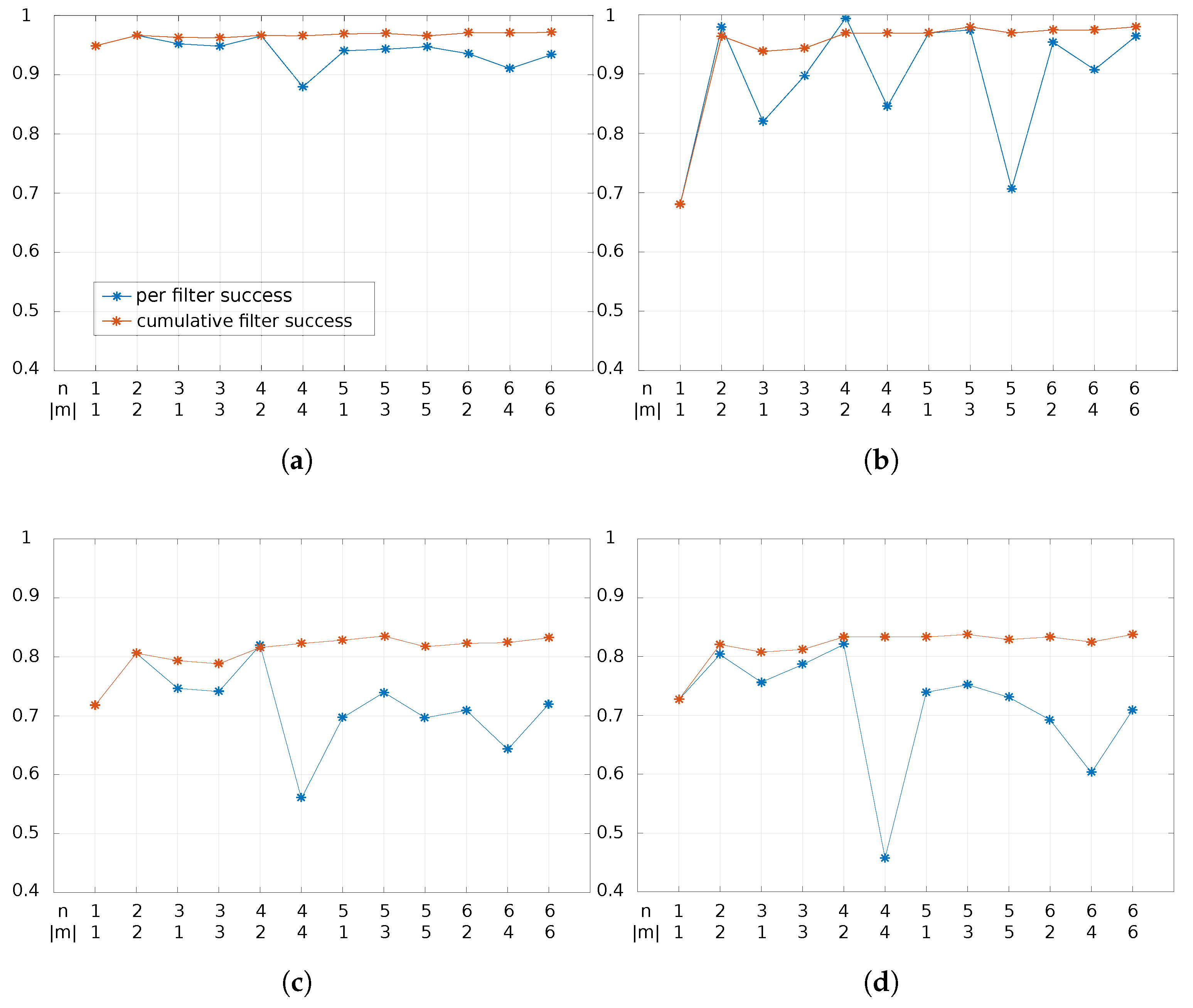
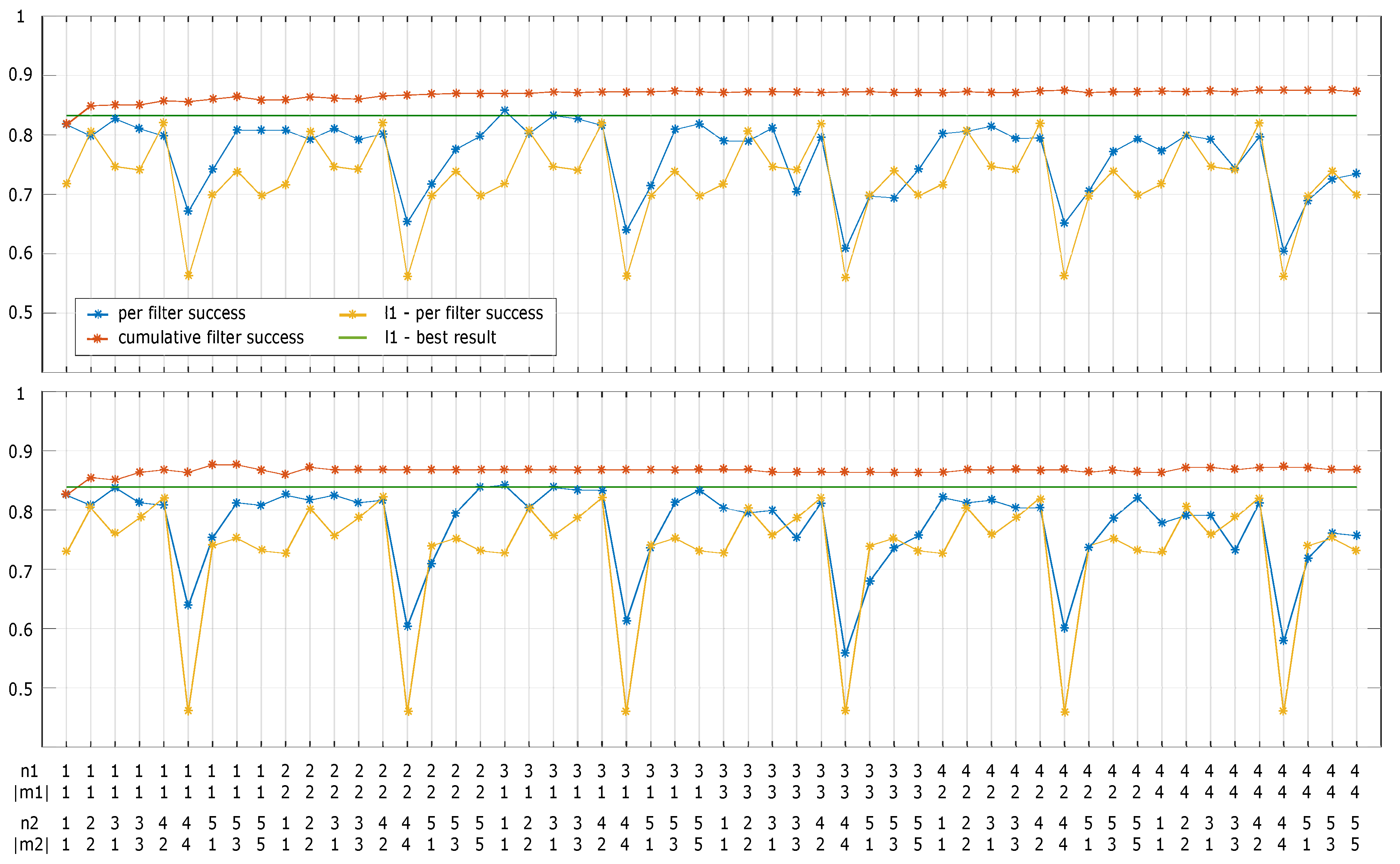
  • Moment degrees and filter sizes used in LZM transformations.
The parameter values used for each dataset are given in Table 5. These values are different because the resolutions of the images presented in the datasets are very different from each other. There are too many low-resolution images in SCface, since the images of the moving persons are recorded at different distances with surveillance cameras. In order to ensure that the image distortions on the face images are not excessive, the face images were used in only three different sizes in the experiments performed with this dataset. In FERET and LFW, the quality of the images is better and therefore five different scales were used to reveal the details in the faces better.
An image can be reconstructed using its own Zernike moments. As the moment degree used increases while the Zernike moments are calculated, the error level of the reconstructed image decreases [80]. In other words, the details of an image can be better encoded by increasing the moment degree. In the experiments performed with FERET, LFW, and SCface-Vis (DayTime protocol), the moment degree was four in both transformations. However, in the experiments performed with SCface-IR (NightTime protocol), the moment degree was one in the first transformation and four in the second transformation. The reason for this situation is that there are fewer details about the faces in the images in SCface-IR. In the first transformation, when low-resolution face images were encoded by taking the moment degree small, intra-class similarities and between-class differences were better preserved. When the moment degree was selected larger, the similarities between the classes increased because there was less distinguishing information to be encoded in the images. While five was used as the filter size in both LZM transformations for FERET, seven was used for other datasets. FERET consists of images obtained from controlled environments, and the images in this dataset have better resolution than the other datasets used in this study. Hence, the area to be locally encoded was kept narrower, so that the details of the face images were more discriminatively encoded. Since the other datasets consist of images from uncontrolled environments, the details in the images have less distinguishing information. Therefore, larger regions were encoded using a larger filter size for these datasets.
In Table 5, we provide the execution time for each different setting to extract features from a face image. When calculating execution times, we did not include the time spent on dimensionality reduction operations in order to clearly see the effect of the parameter values used on execution time. It is possible to reduce the given feature extraction times with a careful implementation and using parallel programming techniques. We have implemented MS-LZM using C++ with OpenCV library, and performed the experiments on a PC with Intel Core i7-3930K CPU and 40 GB RAM.
With the LZM transformation, the desired number of filters can be obtained according to the selected moment degree and number of repetitions. Since the characteristics of these filters are different from each other, different features of face images are extracted with each filter. In this study, all the filters obtained according to the used moment degree were used to construct the feature vectors. Instead of using all filters, using a suitable optimization method, a subset of the filters can be selected that enables the extraction of more distinctive features, and thus better results are likely to be obtained.

5. Conclusions

In this study, we introduced a face recognition scheme using the LZM transformation. The two most important issues for successful face recognition, especially for face images obtained from uncontrolled environments, are the used image descriptor and the designed face recognition scheme. In MS-LZM, which is proposed in this work, the descriptors are obtained using complex images generated by LZM transformation. First, an image pyramid is created for each face image to reveal both local and global properties of the face images. Then, a cascaded LZM transformation is applied to each image in this pyramid. With the first transformation, undesirable conditions such as illumination and blur effects are removed as much as possible. On the LZM images obtained as a result of the second transformation, phase-magnitude histograms (PMH) are calculated around the facial points.
In previous face recognition studies performed with LZM transformation, only face identification or verification problem was taken into consideration. In this study, for both of these problem, we proposed an unsupervised face recognition scheme and achieved high performance on FERET, LFW, and SCface datasets. Each of the datasets used has different characteristics than the others. Since FERET contains a single image for each person in the gallery set, the results for this dataset showed the single sample per person success of MS-LZM. LFW is a popular dataset which consists of unconstrained face images and is used for the verification problem. The last dataset, SCface, was created using images taken from surveillance cameras. Using this dataset, MS-LZM was measured for both low-resolution images and for infrared images. Experimental results showed that our method outperformed state-of-the-art methods on FERET and SCface datasets, and the results obtained for LFW were comparable to the best known results. Taking these results into consideration, it can be easily concluded that MS-LZM is a powerful method that can be used to solve face identification and verification problems encountered in real-world applications.

Author Contributions

E.B. and M.G. conceived and designed the experiments; E.B. performed the experiments and wrote the paper; M.E.K. analyzed the results, guided the full text and revised the manuscript.

Acknowledgments

This work was supported by The Scientific and Technological Research Council of Turkey with the grant number 112E201.

Conflicts of Interest

The authors declare no conflict of interest.

References

  1. Shnain, N.A.; Hussain, Z.M.; Lu, S.F. A feature-based structural measure: An image similarity measure for face recognition. Appl. Sci. 2017, 7, 786. [Google Scholar] [CrossRef]
  2. Ding, C.; Choi, J.; Tao, D.; Davis, L.S. Multi-directional multi-level dual-cross patterns for robust face recognition. IEEE Trans. Pattern Anal. Mach. Intell. 2016, 38, 518–531. [Google Scholar] [CrossRef] [PubMed]
  3. Barr, J.R.; Bowyer, K.W.; Flynn, P.J.; Biswas, S. Face recognition from video: A review. Int. J. Pattern Recognit. Artif. Intell. 2012, 26, 1266002. [Google Scholar] [CrossRef]
  4. Yi, D.; Lei, Z.; Li, S.Z. Shared representation learning for heterogenous face recognition. In Proceedings of the IEEE 2015 11th International Conference and Workshops on Automatic Face and Gesture Recognition (FG), Ljubljana, Slovenia, 4–8 May 2015; Volume 1, pp. 1–7. [Google Scholar]
  5. Marcolin, F.; Vezzetti, E. Novel descriptors for geometrical 3D face analysis. Multimed. Tools Appl. 2017, 76, 13805–13834. [Google Scholar] [CrossRef]
  6. Moos, S.; Marcolin, F.; Tornincasa, S.; Vezzetti, E.; Violante, M.G.; Fracastoro, G.; Speranza, D.; Padula, F. Cleft lip pathology diagnosis and foetal landmark extraction via 3D geometrical analysis. Int. J. Interact. Des. Manuf. IJIDeM 2017, 11, 1–18. [Google Scholar] [CrossRef]
  7. Taigman, Y.; Yang, M.; Ranzato, M.; Wolf, L. Deepface: Closing the gap to human-level performance in face verification. In Proceedings of the IEEE Conference on Computer Vision and Pattern Recognition, Columbus, OH, USA, 24–27 June 2014; pp. 1701–1708. [Google Scholar]
  8. Masi, I.; Rawls, S.; Medioni, G.; Natarajan, P. Pose-aware face recognition in the wild. In Proceedings of the IEEE Conference on Computer Vision and Pattern Recognition, Las Vegas, NV, USA, 27–30 June 2016; pp. 4838–4846. [Google Scholar]
  9. Sarfraz, M.S.; Stiefelhagen, R. Deep Perceptual Mapping for Cross-Modal Face Recognition. Int. J. Comput. Vis. 2016, 122, 426–438. [Google Scholar] [CrossRef]
  10. Xi, M.; Chen, L.; Polajnar, D.; Tong, W. Local binary pattern network: A deep learning approach for face recognition. In Proceedings of the 2016 IEEE International Conference on Image Processing (ICIP), Phoenix, AZ, USA, 25–28 September 2016; pp. 3224–3228. [Google Scholar]
  11. Turk, M.; Pentland, A. Eigenfaces for recognition. J. Cognit. Neurosci. 1991, 3, 71–86. [Google Scholar] [CrossRef] [PubMed]
  12. Belhumeur, P.N.; Hespanha, J.P.; Kriegman, D.J. Eigenfaces vs. fisherfaces: Recognition using class specific linear projection. IEEE Trans. Pattern Anal. Mach. Intell. 1997, 19, 711–720. [Google Scholar] [CrossRef]
  13. Bartlett, M.S.; Movellan, J.R.; Sejnowski, T.J. Face recognition by independent component analysis. IEEE Trans. Neural Netw. 2002, 13, 1450–1464. [Google Scholar] [CrossRef] [PubMed]
  14. Bereta, M.; Pedrycz, W.; Reformat, M. Local descriptors and similarity measures for frontal face recognition: A comparative analysis. J. Vis. Commun. Image Represent. 2013, 24, 1213–1231. [Google Scholar] [CrossRef]
  15. Ahonen, T.; Hadid, A.; Pietikainen, M. Face description with local binary patterns: Application to face recognition. IEEE Trans. Pattern Anal. Mach. Intell. 2006, 28, 2037–2041. [Google Scholar] [CrossRef] [PubMed]
  16. Jin, H.; Liu, Q.; Lu, H.; Tong, X. Face detection using improved LBP under Bayesian framework. In Proceedings of the Third International Conference on Image and Graphics (ICIG’04), Hong Kong, China, 18–20 December 2004; pp. 306–309. [Google Scholar]
  17. Liao, S.; Zhu, X.; Lei, Z.; Zhang, L.; Li, S.Z. Learning multi-scale block local binary patterns for face recognition. In Proceedings of the International Conference on Biometrics, Seoul, Korea, 27–29 August 2007; Springer: Berlin, Germany, 2007; pp. 828–837. [Google Scholar]
  18. Wolf, L.; Hassner, T.; Taigman, Y. Effective unconstrained face recognition by combining multiple descriptors and learned background statistics. IEEE Trans. Pattern Anal. Mach. Intell. 2011, 33, 1978–1990. [Google Scholar] [CrossRef] [PubMed]
  19. Guo, Z.; Zhang, L.; Zhang, D. A completed modeling of local binary pattern operator for texture classification. IEEE Trans. Image Process. 2010, 19, 1657–1663. [Google Scholar] [PubMed]
  20. Tan, X.; Triggs, B. Enhanced local texture feature sets for face recognition under difficult lighting conditions. IEEE Trans. Image Process. 2010, 19, 1635–1650. [Google Scholar] [PubMed]
  21. Zhang, B.; Gao, Y.; Zhao, S.; Liu, J. Local derivative pattern versus local binary pattern: face recognition with high-order local pattern descriptor. IEEE Trans. Image Process. 2010, 19, 533–544. [Google Scholar] [CrossRef] [PubMed]
  22. Daugman, J.G. Uncertainty relation for resolution in space, spatial frequency, and orientation optimized by two-dimensional visual cortical filters. JOSA A 1985, 2, 1160–1169. [Google Scholar] [CrossRef]
  23. Dalal, N.; Triggs, B. Histograms of oriented gradients for human detection. In Proceedings of the IEEE Computer Society Conference on Computer Vision and Pattern Recognition (CVPR 2005), San Diego, CA, USA, 20–25 June 2005; Volume 1, pp. 886–893. [Google Scholar]
  24. Lowe, D.G. Distinctive image features from scale-invariant keypoints. Int. J. Comput. Vis. 2004, 60, 91–110. [Google Scholar] [CrossRef]
  25. Vu, N.S.; Caplier, A. Enhanced patterns of oriented edge magnitudes for face recognition and image matching. IEEE Trans. Image Process. 2012, 21, 1352–1365. [Google Scholar] [PubMed]
  26. Ul Hussain, S.; Triggs, B. Visual recognition using local quantized patterns. In Proceedings of the Computer Vision (ECCV 2012), Florence, Italy, 7–13 October 2012; Springer: Berlin, Germany, 2012; pp. 716–729. [Google Scholar]
  27. Teague, M.R. Image analysis via the general theory of moments. JOSA 1980, 70, 920–930. [Google Scholar] [CrossRef]
  28. Zhai, H.L.; Di Hu, F.; Huang, X.Y.; Chen, J.H. The application of digital image recognition to the analysis of two-dimensional fingerprints. Anal. Chim. Acta 2010, 657, 131–135. [Google Scholar] [CrossRef] [PubMed]
  29. Kan, C.; Srinath, M.D. Invariant character recognition with Zernike and orthogonal Fourier–Mellin moments. Pattern Recognit. 2002, 35, 143–154. [Google Scholar] [CrossRef]
  30. Tan, C.W.; Kumar, A. Accurate iris recognition at a distance using stabilized iris encoding and Zernike moments phase features. IEEE Trans. Image Process. 2014, 23, 3962–3974. [Google Scholar] [CrossRef] [PubMed]
  31. Foon, N.H.; Pang, Y.H.; Jin, A.T.B.; Ling, D.N.C. An efficient method for human face recognition using wavelet transform and Zernike moments. In Proceedings of the IEEE International Conference on Computer Graphics, Imaging and Visualization (CGIV 2004), Penang, Malaysia, 2 July 2004; pp. 65–69. [Google Scholar]
  32. Laine, A.; Fan, J. Texture classification by wavelet packet signatures. IEEE Trans. Pattern Anal. Mach. Intell. 1993, 15, 1186–1191. [Google Scholar] [CrossRef]
  33. Ouanan, H.; Ouanan, M.; Aksasse, B. Gabor-zernike features based face recognition scheme. Int. J. Imaging Robot 2015, 16, 118–131. [Google Scholar]
  34. Fathi, A.; Alirezazadeh, P.; Abdali-Mohammadi, F. A new Global-Gabor-Zernike feature descriptor and its application to face recognition. J. Vis. Commun. Image Represent. 2016, 38, 65–72. [Google Scholar] [CrossRef]
  35. Majeed, S. Face recognition using fusion of Local Binary Pattern and Zernike moments. In Proceedings of the IEEE International Conference on Power Electronics, Intelligent Control and Energy Systems (ICPEICES), Delhi, India, 4–6 July 2016; pp. 1–5. [Google Scholar]
  36. Singh, C.; Walia, E.; Mittal, N. Fusion of Zernike Moments and SIFT Features for Improved Face Recognition. In Proceedings of the International Conference on Recent Advances and Future Trends in Information Technology, Punjab, India, 21–23 March 2012; pp. 26–31. [Google Scholar]
  37. Huang, R.; Du, M.; Me, D. A human face recognition approach based on spatially weighted pseudo-Zernike moments. In Proceedings of the IEEE International Joint Conference on Neural Networks (IEEE World Congress on Computational Intelligence) (IJCNN 2008), Hong Kong, China, 1–8 June 2008; pp. 1604–1608. [Google Scholar]
  38. Kanan, H.R.; Faez, K.; Gao, Y. Face recognition using adaptively weighted patch PZM array from a single exemplar image per person. Pattern Recognit. 2008, 41, 3799–3812. [Google Scholar] [CrossRef]
  39. Sarıyanidi, E.; Dağlı, V.; Tek, S.C.; Tunc, B.; Gökmen, M. Local Zernike Moments: A new representation for face recognition. In Proceedings of the IEEE 2012 19th IEEE International Conference on Image Processing (ICIP), Orlando, FL, USA, 30 September–3 October 2012; pp. 585–588. [Google Scholar]
  40. Alasag, T.; Gokmen, M. Face recognition in low resolution images by using local Zernike moments. In Proceedings of the International Conference on Machine Vision and Machine Learning, Beijing, China, 21–26 June 2014; pp. 1–7. [Google Scholar]
  41. Kahraman, S.E.; Gokmen, M. Face pair matching with Local Zernike Moments and L2-Norm metric learning. In Proceedings of the 2014 22nd IEEE Signal Processing and Communications Applications Conference (SIU), Trabzon, Turkey, 23–25 April 2014; pp. 1524–1527. [Google Scholar]
  42. Basaran, E.; Gokmen, M. An Efficient Face Recognition Scheme Using Local Zernike Moments (LZM) Patterns. In Proceedings of the Asian Conference on Computer Vision, Singapore, 1–2 November 2014; Springer: Berlin, Germany, 2014; pp. 710–724. [Google Scholar]
  43. Sun, X.; Fu, X.; Shao, Z.; Shang, Y.; Ding, H. Local Zernike Moment and Multiscale Patch-Based LPQ for Face Recognition. In Proceedings of 2016 Chinese Intelligent Systems Conference; Springer: Berlin, Germany, 2016; pp. 19–27. [Google Scholar]
  44. Sariyanidi, E.; Gunes, H.; Gökmen, M.; Cavallaro, A. Local Zernike Moment Representation for Facial Affect Recognition. In Proceedings of the British Machine Vision Conference, Bristol, 9–13 September 2013. [Google Scholar]
  45. Gazioğlu, B.S.A.; Gökmen, M. Facial Expression Recognition from Still Images. In Proceedings of the International Conference on Augmented Cognition, Vancouver, BC, Canada, 9–14 July 2017; Springer: Berlin, Germany, 2017; pp. 413–428. [Google Scholar]
  46. Nguyen, H.T.; Caplier, A. Local patterns of gradients for face recognition. IEEE Trans. Inf. Forensics Secur. 2015, 10, 1739–1751. [Google Scholar] [CrossRef]
  47. Xie, S.; Shan, S.; Chen, X.; Chen, J. Fusing local patterns of gabor magnitude and phase for face recognition. IEEE Trans. Image Process. 2010, 19, 1349–1361. [Google Scholar] [PubMed]
  48. Chen, D.; Cao, X.; Wen, F.; Sun, J. Blessing of dimensionality: High-dimensional feature and its efficient compression for face verification. In Proceedings of the IEEE Conference on Computer Vision and Pattern Recognition, Portland, OR, USA, 23–28 June 2013; pp. 3025–3032. [Google Scholar]
  49. Zhu, X.; Lei, Z.; Yan, J.; Yi, D.; Li, S.Z. High-fidelity pose and expression normalization for face recognition in the wild. In Proceedings of the IEEE Conference on Computer Vision and Pattern Recognition, Boston, MA, USA, 7–12 June 2015; pp. 787–796. [Google Scholar]
  50. Su, Y.; Shan, S.; Chen, X.; Gao, W. Hierarchical ensemble of global and local classifiers for face recognition. IEEE Trans. Image Process. 2009, 18, 1885–1896. [Google Scholar] [CrossRef] [PubMed]
  51. Deng, W.; Hu, J.; Guo, J. Gabor-eigen-whiten-cosine: A robust scheme for face recognition. In Proceedings of the International Workshop on Analysis and Modeling of Faces and Gestures, Beijing, China, 16 October 2005; Springer: Berlin, Germany, 2005; pp. 336–349. [Google Scholar]
  52. Schroff, F.; Kalenichenko, D.; Philbin, J. Facenet: A unified embedding for face recognition and clustering. In Proceedings of the IEEE Conference on Computer Vision and Pattern Recognition, Boston, MA, USA, 7–12 June 2015; pp. 815–823. [Google Scholar]
  53. Başaran, E.; Gökmen, M. Face recognition with Local Zernike Moments features around landmarks. In Proceedings of the IEEE 2016 24th Signal Processing and Communication Application Conference (SIU), Zonguldak, Turkey, 16–19 May 2016; pp. 2089–2092. [Google Scholar]
  54. Phillips, P.J.; Moon, H.; Rizvi, S.A.; Rauss, P.J. The FERET evaluation methodology for face-recognition algorithms. IEEE Trans. Pattern Anal. Mach. Intell. 2000, 22, 1090–1104. [Google Scholar] [CrossRef]
  55. Huang, G.B.; Ramesh, M.; Berg, T.; Learned-Miller, E. Labeled Faces in the Wild: A Database for Studying Face Recognition in Unconstrained Environments; Technical Report 07-49; University of Massachusetts: Amherst, MA, USA, 2007. [Google Scholar]
  56. Grgic, M.; Delac, K.; Grgic, S. SCface–surveillance cameras face database. Multimed. Tools Appl. 2011, 51, 863–879. [Google Scholar] [CrossRef]
  57. Chong, C.W.; Raveendran, P.; Mukundan, R. A comparative analysis of algorithms for fast computation of Zernike moments. Pattern Recognit. 2003, 36, 731–742. [Google Scholar] [CrossRef]
  58. King, D.E. Dlib-ml: A Machine Learning Toolkit. J. Mach. Learn. Res. 2009, 10, 1755–1758. [Google Scholar]
  59. Kazemi, V.; Sullivan, J. One millisecond face alignment with an ensemble of regression trees. In Proceedings of the IEEE Conference on Computer Vision and Pattern Recognition, Columbus, OH, USA, 24–27 June 2014; pp. 1867–1874. [Google Scholar]
  60. Julesz, B. Textons, the elements of texture perception, and their interactions. Nature 1981, 290, 91–97. [Google Scholar] [CrossRef] [PubMed]
  61. Howard, I.P.; Rogers, B.J. Binocular Vision and Stereopsis; Oxford University Press: Oxford, MS, USA, 1995. [Google Scholar]
  62. Pentland, A. Experiments with Eigenfaces; M.I.T. Media Lab Vision and Modeling Group Technical Report; Vision and Modeling Group, Media Laboratory, Massachusetts Institute of Technology: Cambridge, MA, USA, 1992. [Google Scholar]
  63. Moon, H.; Phillips, P.J. Computational and performance aspects of PCA-based face-recognition algorithms. Perception 2001, 30, 303–321. [Google Scholar] [CrossRef] [PubMed]
  64. Cament, L.A.; Castillo, L.E.; Perez, J.P.; Galdames, F.J.; Perez, C.A. Fusion of local normalization and Gabor entropy weighted features for face identification. Pattern Recognit. 2014, 47, 568–577. [Google Scholar] [CrossRef]
  65. Vu, N.S. Exploring patterns of gradient orientations and magnitudes for face recognition. IEEE Trans. Inf. Forensics Secur. 2013, 8, 295–304. [Google Scholar] [CrossRef]
  66. Chai, Z.; Sun, Z.; Mendez-Vazquez, H.; He, R.; Tan, T. Gabor ordinal measures for face recognition. IEEE Trans. Inf. Forensics Secur. 2014, 9, 14–26. [Google Scholar] [CrossRef]
  67. Viola, P.; Jones, M.J. Robust real-time face detection. Int. J. Comput. Vis. 2004, 57, 137–154. [Google Scholar] [CrossRef]
  68. Sharma, G.; Jurie, F. Local higher-order statistics (LHS) describing images with statistics of local non-binarized pixel patterns. Comput. Vis. Image Underst. 2016, 142, 13–22. [Google Scholar] [CrossRef]
  69. Arashloo, S.R.; Kittler, J. Efficient processing of MRFs for unconstrained-pose face recognition. In Proceedings of the 2013 IEEE Sixth International Conference on Biometrics: Theory, Applications and Systems (BTAS), Arlington, VA, USA, 29 September–2 October 2013; pp. 1–8. [Google Scholar]
  70. Ylioinas, J.; Kannala, J.; Hadid, A.; Pietikäinen, M. Face recognition using smoothed high-dimensional representation. In Proceedings of the Scandinavian Conference on Image Analysis, Copenhagen, Denmark, 15–17 June 2015; Springer: Berlin, Germany, 2015; pp. 516–529. [Google Scholar]
  71. Yi, D.; Lei, Z.; Li, S.Z. Towards pose robust face recognition. In Proceedings of the IEEE Conference on Computer Vision and Pattern Recognition, Portland, OR, USA, 23–28 June 2013; pp. 3539–3545. [Google Scholar]
  72. Juefei-Xu, F.; Luu, K.; Savvides, M. Spartans: Single-sample periocular-based alignment-robust recognition technique applied to non-frontal scenarios. IEEE Trans. Image Process. 2015, 24, 4780–4795. [Google Scholar] [CrossRef] [PubMed]
  73. Arashloo, S.R.; Kittler, J. Class-specific kernel fusion of multiple descriptors for face verification using multiscale binarised statistical image features. IEEE Trans. Inf. Forensics Secur. 2014, 9, 2100–2109. [Google Scholar] [CrossRef]
  74. Chan, C.H.; Kittler, J.; Messer, K. Multi-scale local binary pattern histograms for face recognition. In Proceedings of the International Conference on Biometrics, Seoul, Korea, 27–29 August 2007; Springer: Berlin, Germany, 2007; pp. 809–818. [Google Scholar]
  75. Tahir, M.A.; Chan, C.H.; Kittler, J.; Bouridane, A. Face recognition using multi-scale local phase quantisation and linear regression classifier. In Proceedings of the IEEE 2011 18th IEEE International Conference on Image Processing (ICIP), Brussels, Belgium, 11–14 September 2011; pp. 765–768. [Google Scholar]
  76. Kannala, J.; Rahtu, E. Bsif: Binarized statistical image features. In Proceedings of the IEEE 2012 21st International Conference on Pattern Recognition (ICPR), Tsukuba, Japan, 11–15 November 2012; pp. 1363–1366. [Google Scholar]
  77. Peng, Y.; Gökberk, B.; Spreeuwers, L.; Veldhuis, R. An evaluation of super-resolution for face recognition. In Proceedings of the 33rd WIC Symposium on Information Theory in the Benelux, Enschede, The Netherlands, 24–25 May 2012; pp. 36–43. [Google Scholar]
  78. Wilman, W.W.Z.; Yuen, P.C. Very low resolution face recognition problem. In Proceedings of the 2010 Fourth IEEE International Conference on Biometrics: Theory, Applications and Systems (BTAS), Arlington, VA, USA, 27–29 September 2010; pp. 1–6. [Google Scholar] [CrossRef]
  79. Nguyen, H.T.; Caplier, A. Elliptical local binary patterns for face recognition. In Proceedings of the Asian Conference on Computer Vision, Daejeon, Korea, 5–6 November 2012; Springer: Berlin, Germany, 2012; pp. 85–96. [Google Scholar]
  80. Khotanzad, A.; Hong, Y.H. Rotation invariant image recognition using features selected via a systematic method. Pattern Recognit. 1990, 23, 1089–1101. [Google Scholar] [CrossRef]
Figure 1. Zernike polynomials calculated using values up to n = 5 (left), and 7 × 7 local Zernike moments (LZM) filters corresponding to these polynomials (right). Negative values of m represent imaginary, while positive values represent real components.
Applsci 08 00827 g001
Figure 2. Real and imaginary components obtained for a face image using the LZM filters given in Figure 1.
Applsci 08 00827 g002
Figure 3. Steps of the proposed multi-scale feature extraction scheme using LZM components. Shows the process of construction of a feature vector for only a facial point.
Applsci 08 00827 g003
Figure 4. (a) Sixty-eight facial points detected using the algorithm suggested by Kazemi et al. [59]; (b) 21 facial points used to extract facial features.
Applsci 08 00827 g004
Figure 5. Sample face images from the FERET dataset. Images were aligned using a similarity transformation and cropped.
Applsci 08 00827 g005
Figure 6. Identification rates obtained for (a) Fb; (b) Fc; (c) Dup1; and (d) Dup2, using single LZM transformation. Blue markings indicate the performance per filter, and red markings indicate the cumulative performance.
Applsci 08 00827 g006
Figure 7. Per-filter and cumulative filter identification rates obtained for Dup1 (top) and Dup2 (bottom), using single (yellow markings and green line) and cascaded LZM (red and blue markings) transformations. Blue markings indicate the performance per filter, and red markings indicate the cumulative performance. Green line and yellow markings indicate the best results and the performance per filter given in Figure 6, respectively.
Applsci 08 00827 g007
Figure 8. Dup2 results calculated using cascaded and combined filters which were obtained using different n and | m | values.
Applsci 08 00827 g008
Figure 9. Sample face images from Labeled Faces in the Wild (LFW). The first, third and fifth columns show original images, and the second, fourth, and sixth columns show frontalized images.
Applsci 08 00827 g009
Figure 10. Images from SCface. (a) In visible and (b) in infra-red spectrum. In the first column, mugshot gallery images are given. In second, third, and fourth columns, the images recorded at distance 1, 2, and 3 are given, respectively.
Applsci 08 00827 g010
Table 1. Identification rates on FERET with state-of-the-art results. MS-LZM: multi-scale local Zernike moments.
MethodFbFcDup1Dup2Avg
LMEGW//LN + LGXP [64]99.910094.791.997.5
s-POEM + POD + WPCA [65]99.710094.994.097.7
GOM [66]99.910095.793.197.9
LMEGW//LN + LGBP [64]99.910095.693.698.0
Basaran et al. [42]99.810096.094.998.2
MDML-DCPs + WPCA [2]99.810096.195.798.3
Basaran et al. [53]99.810097.596.698.8
LPOG + WPCA [46]99.810097.497.098.8
MS-LZM99.710098.197.999.1
Table 2. Verification rates on LFW with state-of-the-art results.
MethodAUC
LHS [68]0.8107
MRF-MLBP [69]0.8994
SA-BSIF + WPCA [70]0.9318
LBPNet [10]0.9404
Pose Adaptive Filter (PAF) [71]0.9405
Spartans [72]0.9428
MRF-Fusion-CSKDA [73]0.9894
MS-LZM0.9515
Table 3. Results of SCface DayTime protocol with state-of-the-art results.
ProbePCA [56]SR [77]DSR [78]ELBP [79]LPOG [46]MS-LZM
cam1_12.3N/AN/A43.169.272.3
cam1_27.756.273.175.4
cam1_35.445.447.742.3
cam2_13.136.957.762.3
cam2_27.750.866.274.6
cam2_33.942.348.543.1
cam3_11.534.649.253.9
cam3_23.946.963.180.8
cam3_37.751.554.654.6
cam4_10.732.343.969.2
cam4_23.950.075.482.3
cam4_38.550.858.556.9
cam5_11.536.253.964.6
cam5_27.732.352.364.6
cam5_35.431.538.536.2
Average4.716.420.242.756.862.2
Table 4. Results on the SCface NightTime Protocol with state-of-the-art results.
ProbePCA [56]ELBP [79]LPOG [46]MS-LZM
cam6_11.59.213.121.5
cam6_23.115.423.938.5
cam6_33.925.431.533.1
cam7_10.713.117.727.7
cam7_25.413.120.034.6
cam7_34.613.919.225.4
Average3.215.020.930.1
Table 5. Parameter values used for each dataset and feature extraction time for different settings.
Datasetn1n2k1k2#ScalesTime
FERET445550.82 s
LFW447750.95 s
SCface-Vis447730.39 s
SCface-IR147730.10 s
(n1, k1) and (n2, k2) parameter pairs are for first and second LZM transformation, respectively. IR: infrared spectrum; Vis: visible spectrum.

