1. Introduction
Massive MIMO (multiple-input multiple-output) technology is one of the key technologies of next-generation mobile cellular networks, which can form a massive antenna array by providing a large number of antennas at the cell base station. It will greatly improve the channel capacity and spectrum utilization and has become a hotspot in the field of wireless communications in recent years [
1]. In a massive MIMO system, a precise channel state information (CSI) is critical, which is directly related to the system signal detection, beamforming, resource allocation and so on. The number of base station antennas in massive MIMO systems has reached hundreds of thousands, which greatly deepens the complexity of system data processing. Therefore, in order to make full use of the potential advantages of massive MIMO technology, the more efficient and low complexity channel estimation algorithms are worthy of further study. Massive MIMO has various merits over the conventional MIMO. First, it uses a large number of antennas at the BS due to which the simplest coherent-combiner and linear-precoder can be used for signal processing such MF or ZF. Second, increasing the number of antennas increases the system capacity substantially using the channel-reciprocity features and without increasing feedback-overhead. Third, the reduced power benefits in the uplink/downlink (UL/DL) provide the feasibility to shrink the cell-size, which can be used in micro and pico-cells.
The massive multi-input multi-output (MIMO) system has doubled the capacity of the communication system without increasing the signal bandwidth and signal transmission power and is regarded as the core technology of 5G wireless communication. Channel estimation is the key technology in the physical layer of massive MIMO systems. Its accuracy directly affects the system performance under fading channels.
In massive MIMO systems, accurate Channel State Information (CSI) is required to utilize the full potential of MIMO systems [
2,
3]. However, such accurate CSI is not available in real communication environment [
4]. With the increasing number of antennas, the receiver has to estimate more channel coefficients, which effectively increases the pilot overhead, computational complexity and reduces the overall throughput of the system [
5]. This is a challenging issue which has been addressed in [
3,
4,
5,
6]. Literature [
7,
8,
9,
10,
11,
12,
13,
14,
15] shows that the massive MIMO channel has sparse characteristics which can be utilized for computationally-efficient channel estimation. Classical channel estimation methods include least-square (LS) algorithm [
16], minimum mean-squared error (MMSE) algorithm [
17], linear minimum mean square error (LMMSE) [
18] and so on. The actual radio channel has a certain multi-sparseness [
19]. In recent years, a large number of researchers applied compressive sensing to the pilot-aided channel estimation, e.g., in [
20,
21]. Research shows that compressed channel estimation achieves better performance based on the same number of pilots in sparse channels.
Compressed sensing channel estimation algorithms orthogonal matching pursuit (OMP) [
22], regularization orthogonal matching pursuit (ROMP) [
23], and subspace pursuit (SP) [
24] are currently used. The above algorithms need to predict the channel sparsity. However, the channel sparsity in the actual communication environment is usually unknown, which greatly limits the application of the above algorithm. The sparsity adaptive matching pursuit (SAMP) algorithm can recover sparsity-unknown channels [
25], but the algorithm has a high dependence on the iterative steps, resulting in the pursuit of high performance and at the same time, greater computational complexity.
Massive MIMO systems need to deal with a huge amount of data, and the traditional compression-aware channel estimation algorithm is difficult to strike a balance between estimation performance and computational complexity. The literature [
26] shows that in a massive MIMO system, the sub-channels between different transmitting and receiving antenna pairs have the same sparse support set. In [
27], an adaptive and structured subspace pursuit algorithm (ASSP) is proposed for massive MIMO channel estimation. Because of its step-by-step approach, achieving sparseness adaptation and the deficiencies have been underestimated, and the computational complexity is high.
This paper proposes a sparsity-adaptive channel estimation algorithm based on the joint sparsity feature of a massive MIMO channel. When the channel sparsity is unknown, a block sparse adaptive channel estimation algorithm is proposed, which is block sparsity adaptive matching pursuit (BSAMP). By setting the threshold and finding the maximum backward difference position, the support set element is preliminarily selected. The element is secondarily selected by regularization to improve the accuracy of the selected element. The proposed solution can be applied to any scenario of the massive MIMO channel in which the sparse attributes are utilized for effective channel estimation. The key factor is to set the threshold value and determine the position of the non-zero elements in the support set. The simulation results show that this method can obtain better channel estimation performance with lower complexity under the condition of unknown sparsity.
Notations: Lowercase and upper-case boldface letters denote vectors and matrices, respectively; , and denote the transpose, conjugate transpose, and inverse of a matrix, respectively.
2. Sparse Multipath Channel Model
In a base station (BS) equipped with
M transmitting antenna MIMO systems, the transmitting end sends orthogonal frequency-division multiplexing (OFDM) signals, and the length of each OFDM signal transmitted by each antenna is
N, where
P(0 <
P <
N) carriers are selected as the pilot for channel estimation, and the channel length
L. The pilot pattern of the
ith transmit antenna is
p(
i),
i = 1, 2, ...,
M, where,
p(
i)∩
p(
j) = ∅, If
i ≠
j. After the channel is transmitted, the receiving end receives the pilot signal corresponding to each antenna as
y(
p(
i)),
i = 1, 2, ...,
M. Abbreviate
y(
p(
i)) as
y(i), the basic channel model can be expressed as:
among them,
D(i) = diag{
p(
i)} is a diagonal array of selected pilot patterns,
m(i) is a Gaussian White Noise with mean 0 and variance σ
2,
F(i) is a
P ×
L sub-matrix of a Fourier, corresponding to the dimensions
N ×
N discrete Fourier transform (DFT) matrix pilot line elements and the first
L columns,
h(i) = [
h(i)(1),
h(i)(2),...,
h(i)(
L)]
T is the channel impulse response (CIR) corresponding to the
ith antenna. Make
A(i) =
D(i)F(i), Then, Equation (1) can be further expressed as:
Definition 1. supp{h(i)} = {l: |h(i) (l) |> pth, 1 ≤ l ≤ L} is the ith sub-channel support set index, and pth is the noise threshold. The research shows that for longer signal transmission distance, the antenna array size of the BS is very small, the delay dispersion characteristics of subchannels between different transmitting and receiving antenna pairs in massive MIMO system are consistent and have approximately the same channel delay. The delay model shows the same sparse support set of sub-channels between different transmitting antennas and users [12], that is: Because the rate of change of channel gain is much larger than the rate of change of delay, the gain coefficients of each subchannel are different, but the positions of nonzero taps of different subchannels are the same, showing a joint sparse characteristic. Based on this characteristic, designing an appropriate recovery algorithm can achieve a more accurate and quick estimate of channel information.
3. Sparse Adaptive Matching Pursuit Algorithm
3.1. Sparseness Estimation
Using compressed sensing to solve channel estimation can be equivalent to solving the following
l0 norm minimum problem.
among them,
is the vector
l0 norm of the vector
h for the number of non-zero elements. Literature [
28] has proved that when satisfied:
Only the channel impulse response (h) can be restored. Among them, spark(A) is the least linearly related column number in matrix A; it is easy to see 2 ≤ spark(A) ≤ rank(A) + 1. Since matrix A is P × L partial Fourier matrix and P < L, then < .
Because of the sparseness of the impulse response of the wireless communication channel, most of the energy is concentrated on a few taps while a small part of the energy distribution is below the noise threshold. The number of non-zero taps is much smaller than the channel length L. Making full use of the sparse characteristics of the channel, we can use fewer pilot symbols to get the ideal channel estimation effect, so as to improve the spectrum utilization. An appropriate amount of pilot overhead satisfies Equation (5), so
Based on the above analysis, the number of non-zero taps in the channel vector does not exceed K, and at least elements can be regarded as noise. Therefore, we first estimate the sparseness and then select the elements within this range. At higher signal-to-noise ratios, since the gain coefficients of the channel taps are higher than the noise amplitudes, the restored vector elements are arranged in descending order. The difference between adjacent elements is then used to determine the number of elements selected for this iteration and to further estimate the sparsity. The elements that precede the largest backward difference are selected for the support set because they may carry channel information.
When the observation matrix satisfies certain conditions, the sparse signal restoration problem can be equivalent to the following convex optimization problem. Define the observation matrix
A, the RIP parameter
δk is the minimum value
δ that satisfies Equation (7):
among them,
is the sparse signal for
k, if
δk < 1, the observation matrix
satisfies the
kth order RIP [
29]. When matrix RIP parameters
δk <
−1, the reconstruction problem can be transformed into the following
l1 norm minimum problem.
Due to partial Fourier matrix RIP parameters
δk <
[
30], the regularization process based on convex optimization is introduced to improve the stability of the algorithm [
23].
3.2. Sparse Multipath Channel Estimation
Aiming at the joint sparseness presented by the massive MIMO channel, the transformed channel vector is defined as
w = [
w1T,
w2T,...,
wLT]
T, where
wi = [
h(1)(
i),
h(2)(
i),...,
h(M)(
i)]
T,
i = 1, 2, ...,
L, the
i sub-block for
w. At this point, the non-zero elements in the converted channel vector will be concentrated [
31]. Correspondingly, the received pilot signal is warped
z = [
z1T,
z2T, ...,
zpT]
T. Among them,
zi = [
y(1)(
i),
y(2)(
i), ...,
y(M)(
i) ]
T,
i = 1, 2, ...,
P. Do the same for noise,
n = [
n1T,
n2T, ...,
nPT]
T, where
ni = [
m(1)(
i),
m(2)(
i), ...,
m(M)(
i)]
T,
i = 1, 2, ...,
P. Considering all transmit antennas, the received signal can be expressed as:
among them,
B = [
B1,
B2, ...,
BL];
Bi = [a
(1)(
i), a
(2)(
i), ..., a
(M)(
i)],
i = 1, 2, ...,
L is the
ith sub-block of matrix
B, a
(M)(
i) is the
ith column of the matrix
A(M). In the case of unknown channel sparsity, the compressed sensing is used to estimate
w in Equation (9), so multiply both sides of Equation (9) simultaneously by
BH, where
BH is the conjugate transpose of the matrix
B.
among them,
I denote
ML ×
ML unit matrix. Due to the matrix
B, there is no strict orthogonality; therefore,
BHB −
I denote a nonzero matrix with a small elemental value. Consider the dispersion of energy caused by the non-orthogonality of the observed matrix
n’ = (
BHB −
I)
w +
BHn, Then, Equation (10) can be expressed as:
During iteration, define an
ML × 1 vector
R.
among them,
r denotes iterative residuals, its initial value is
z, |⋅| represents the absolute value of the elements in
BHr. Now, define the element in vector
T as the sum of the squares of each set of
M elements in the vector
R
where
R(
i) is the
ith element in vector
R,
T(
j) is the
jth element in vector
T. Correct
T Elements in descending order to get the vector
Ts. According to the analysis in
Section 3.1 the upper limit of channel sparsity is
K. After the first iteration, the last
L-
K elements in
Ts are only generated by
n’ in (11). So the energy of the next
L-
K elements is set as the threshold
f. The non-zero tap energy in the channel is greater than the threshold
f. So in
Ts, only elements above this threshold are likely to be included in the support set.
At higher signal-to-noise ratios, since the gain coefficient of the channel tap is higher than the noise amplitude, at each iteration of the algorithm,
Ts of the element amplitude produces a larger rate of change; then the element before this position has to carry channel information. Therefore, calculating the maximum backward difference between adjacent elements determines the number of elements selected in this iteration, and the elements before this position are selected for the support set because they may carry channel information. In order to further improve the accuracy of the selected elements, the regularization process based on convex optimization is adopted to ensure that the selected element energy is larger than the energy of the unselected elements [
23], and the noise is filtered out to support the set.
From the above analysis we can see that the sparseness estimation of BSAMP algorithm first estimates the sparsity upper limit by setting the threshold according to the actual physical characteristics of the channel, that is to say, the maximum sparsity will not exceed the number of pilots so as to ensure that the channel taps will not miss selection. Sparseness is further estimated by finding the maximum difference location in this range to distinguish channel taps and noise. Unlike other compression-aware algorithms, only the influential factors associated with Gaussian white noise are considered BHn. The BSAMP algorithm not only considers BHn but also considers the energy dispersion due to the non-orthogonality of the observation matrix (BHB − I)w impact algorithm performance. In addition, the BSAMP algorithm uses a regularization method to filter the elements in the support set for secondary screening, which improves the accuracy of the support set. Therefore, the BSAMP algorithm has better estimation performance than other algorithms.
The massive MIMO system needs to recover the larger channel dimension, and the sub-channel presents joint sparseness. The BSAMP algorithm takes advantage of channel block sparse features, greatly reducing the number of iterations. In the meantime, there are multiple element-selected support sets in each iteration, and the problem that the traditional step-based adaptive algorithm relies on iterative step-size is avoided. Therefore, the BSAMP algorithm has lower computational complexity.
The specific BSAMP algorithm process is as follows in Algorithm 1.
| Algorithm 1 BSAMP Algorithm |
Input receive pilot signal z, Observation matrix B, The number of antennas M
Output channel estimate h’.
Initialize the block support set location index S1 = ∅, Support set location index S2 = ∅, h’= 0, The threshold f = E {[Ts (i)]2, i = K + 1, K + 2, ..., L}, r = z.
Iteration process
1: Calculate vector T, arrange the elements in T in descending order to obtain a vector Ts and the corresponding index set S1.
2: Select the elements in Ts larger than the threshold f and set the element number to m; if m= 0, exit; otherwise, go to Step 3.
3: Select the vector Ts(1:m + 1) and the maximum backward difference between adjacent elements is labeled as t.
4: Regularize the elements in the vector Ts(1:t). make u = Ts (1:t), J = S1(1:t), All elements in u follows |u(i)| ≤ 2|u(j)|, i, j ∈ J Divided into a number of groups, select the energy of the largest group of a selected support set. The location of the selected elements is indexed V, and if the length of the vector V is U, S2 = S2∪[(V(k) − 1) M + 1: V(k)M], k = 1, 2, L, U .
5: According to the location index S2, find the matrix of the corresponding columns in the observation matrix .
6: Solve the estimated channel using the least square method h’ = .
7: Update the residual r = z − h’, make S1 = ∅, V = ∅
8: Return to Step 1. |
4. Simulation Results
The MATLAB (2017a, MathWorks, Natick, MA, USA, 2017) simulator is used for the analysis.
Table 1 mentioned the main simulation setup parameters for the proposed system. In the simulation, the system has 500 transmit antennas, using 64QAM modulation and low-density parity-check (LDPC) coding (coding efficiency 5/8). Each transmit antenna sends an OFDM signal with a signal length
N of 256, with a cyclic prefix length of 64. The OFDM signals transmitted by each transmitting antenna have 16 pilot symbols, and all the algorithms use the same pilot distribution method. The pilot positions are randomly distributed and the pilots of different antennas are orthogonal to each other. The channel length
L is 60, and the number of channel multipath is a random integer [
5,
8]. The multipath amplitude follows the Rayleigh distribution, and the multipath positions follow a random distribution.
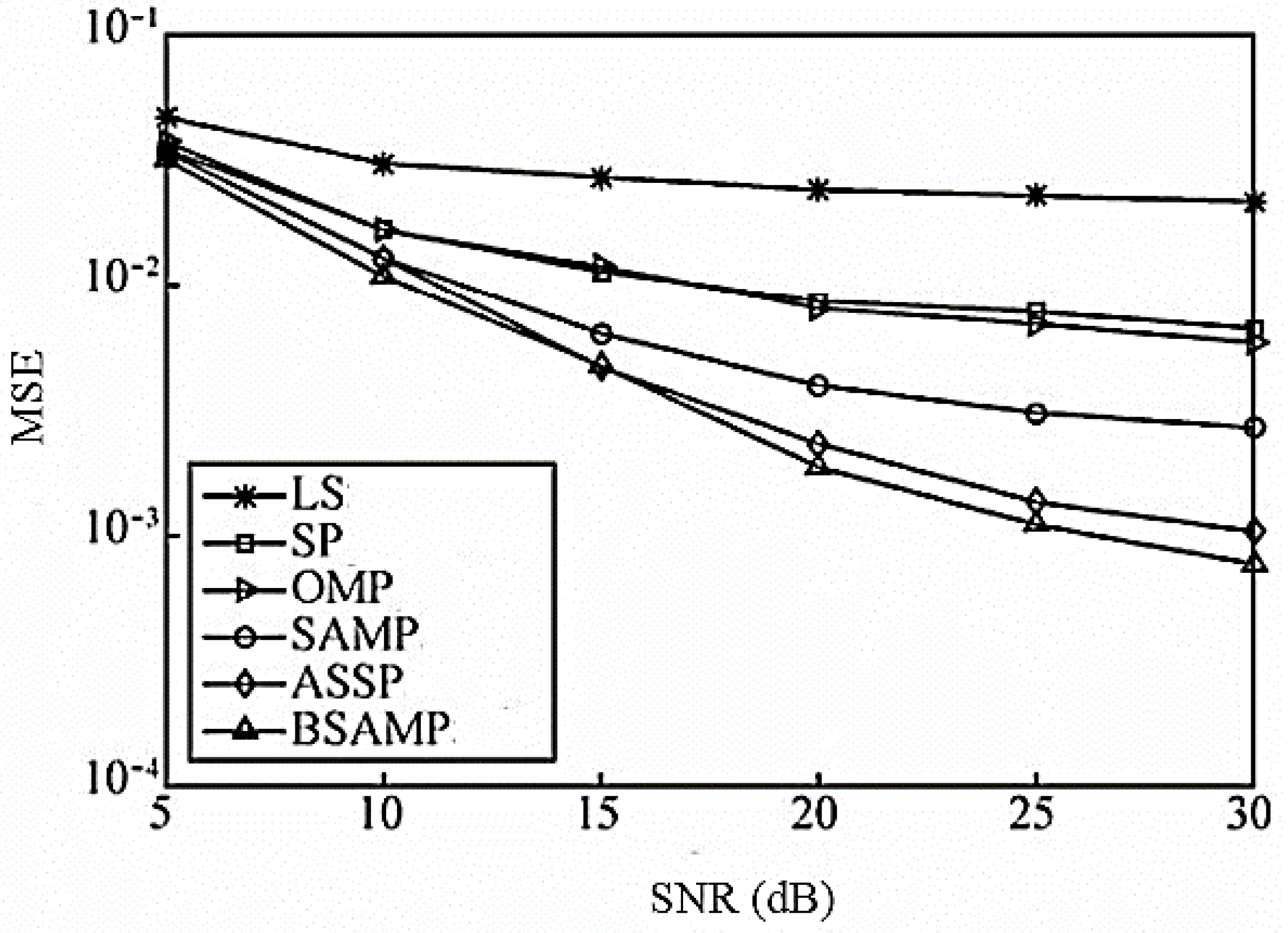
Figure 1 shows the mean square error (MSE) performance of each channel estimation algorithm at different signal-to-noise ratios when the pilot number is 16.
As can be seen from the
Figure 1, the performance of BSAMP algorithm proposed in this paper is superior to other algorithms. This is because the LS algorithm fails when the pilot number is less than the channel length, while the OMP and SP algorithms need to set their iteration times to half the number of pilots when the channel sparsity is unknown, reducing the accuracy of the algorithm. SAMP algorithm and ASSP algorithm do not need prior information such as the sparsity of the channel. However, the SAMP algorithm and the ASSP algorithm realize the adaptive process by using a fixed increment step, which easily causes over-estimation and under-estimation, which is slightly less than the estimation accuracy. The proposed BSAMP algorithm not only considers the effect of Gaussian white noise on the system performance but also considers the energy dispersion caused by the non-orthogonality of the observed matrix, which has better performance than the above algorithm.
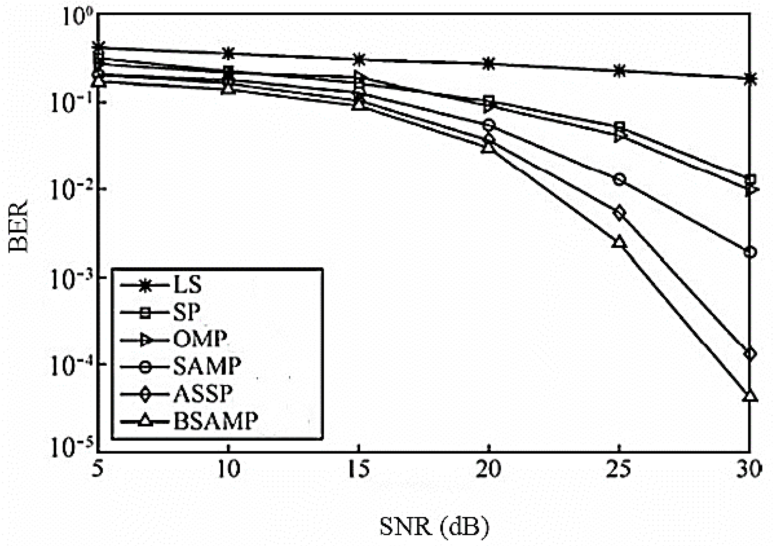
Figure 2 shows the systematic bit error rate (BER) for each channel estimation algorithm at different signal-to-noise ratios when the number of pilots is 16. As can be seen from the Figure, the BSAMP algorithm using the system BER has the best performance. When the SNR is 30 dB, the system BER reaches 4.187 × 10
−5.
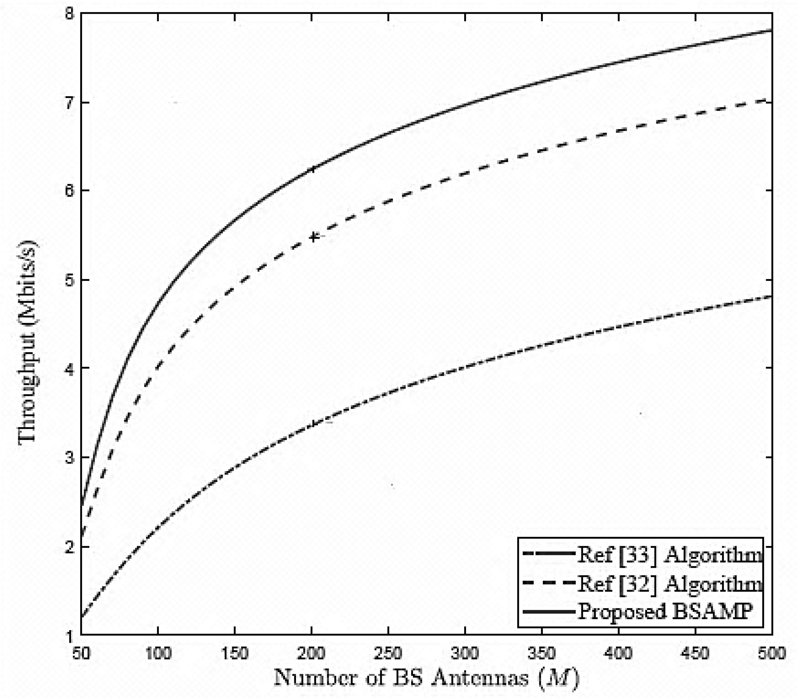
Figure 3 compares the throughput between the proposed BSAMP algorithm with literature [
32,
33] algorithms versus the number of antennas. It is clear from the
Figure 3 that, as the number of antennas (
M) increases, the throughput of all the algorithms improves. Moreover, the proposed BSAMP algorithm outperforms the other algorithms and the rate gap between them increases with increasing number of antennas.
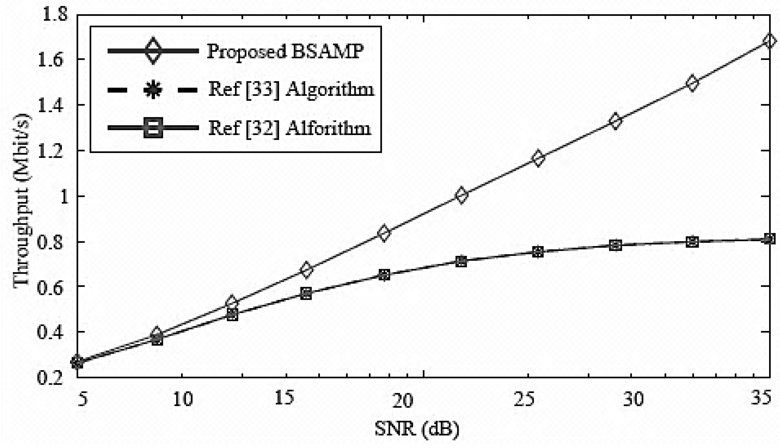
Figure 4 compares the throughput of the proposed BSAMP algorithm with literature [
32,
33] algorithms versus the SNR. It is clear from the
Figure 4 that, as the SNR increases, the throughput of each algorithm increases. Moreover, the proposed BSAMP algorithm shows overall better throughput as compared with the reference [
32,
33] algorithms. Furthermore, the rate gap between the proposed BSAMP algorithm and the literature [
32,
33] algorithms increases as the SNR increases, which makes the BSAMP algorithm superior in low and high SNR communication environments. The throughput levels of literature [
32,
33] are more closely related and show approximately same characteristics for different levels of SNR.
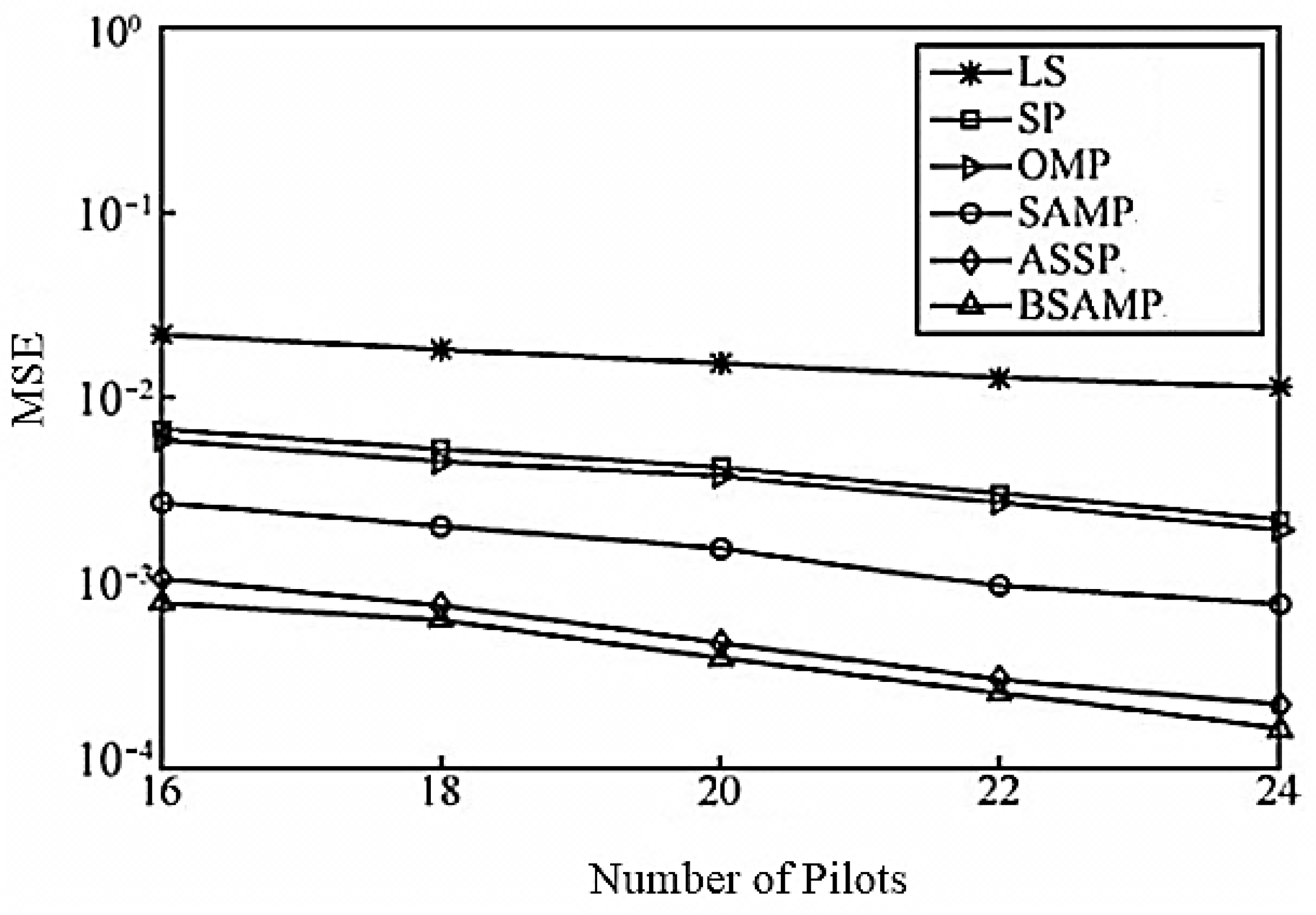
Figure 5 shows the MSE performance of each channel estimation algorithm under a different number of pilots when SNR is 30 dB. As can be seen from the Figure, as the number of pilots increases, the performance of each recovery algorithm is improved. Under the same number of pilots, the ASSP algorithm is significantly better than other channel estimation algorithms due to the joint sparseness of MIMO channels. At the same time, BSAMP does not need to rely on the iterative steps to achieve the sparsity adaptive process. The BSAMP algorithm effectively eliminates the influence on the estimation accuracy due to improper step selection in the iterative process, which has better performance than the ASSP algorithm. When the number of pilots is 16, the performance of the BSAMP algorithm is equivalent to that of ASSP with 18 pilots. On the other hand, the LS shows the worst channel estimation performance while the SP and OMP have approximately similar MSE. The SAMP algorithm indicates better performance than the OMP, SP, and LS but is less effective than the ASSP and BSAMP algorithms as the MSE gap among them increases with increasing number of pilots. In summary, it is concluded from
Figure 3 that, to obtain the required MSE and better channel estimation performance, the LS, SP, OMP, SAMP and ASSP algorithms need more pilots than the proposed BSAMP algorithm, which makes them less effective and application-oriented. Therefore, the proposed BSAMP algorithm shows overall better performance.
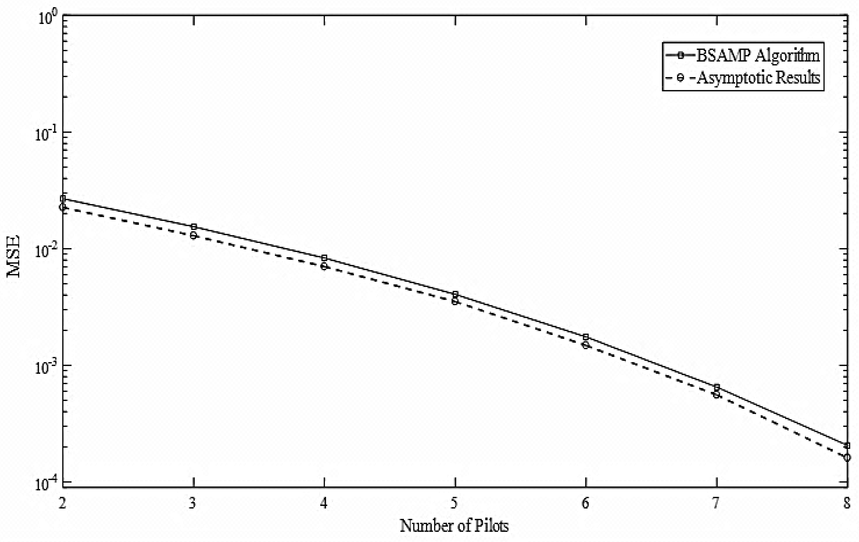
Figure 6 shows the comparison of the proposed BSAMP algorithm and the asymptotic results. It is clear from the figure that the proposed algorithm shows close performance with the asymptotic results which makes it an attractive candidate from the practical perspective in wireless communications.
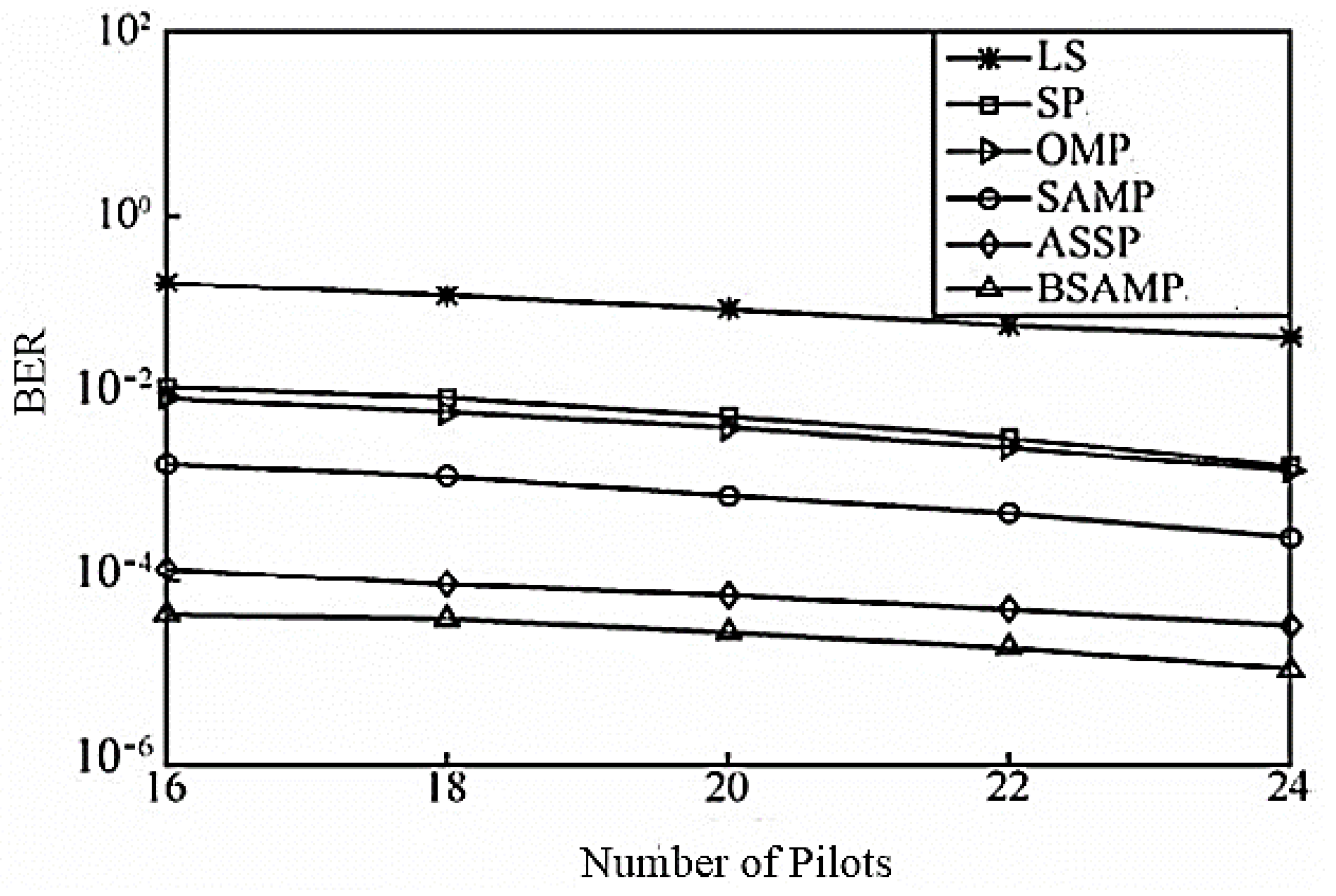
Figure 7 shows the systematic BER of each channel estimation algorithm under different pilots when SNR is 30 dB. As can be seen from the Figure, under the same pilot number, the BSAMP algorithm performance is far superior to that of other algorithms. When the pilot number is 24, the system BER reaches 1.066 × 10
−5.
Table 2 shows the different sparse channel recovery algorithms. It can be seen that the BSAMP algorithm is comparable in computational complexity to the LS algorithm but much lower than other compression aware algorithms. Due to the larger channel vector dimension and unknown channel sparsity, too many iterations result in higher computational complexity for OMP and SP algorithms.
The SAMP algorithm does not take advantage of the joint sparseness of the MIMO channel and gradually approximates the channel sparsity by a fixed step, which takes a lot of time. The ASSP algorithm also has the problem of increasing the iterative step length steadily, but it takes advantage of the joint sparseness of the channel and reduces the computation time compared with SAMP. The BSAMP algorithm proposed in this paper can achieve the sparsity adaptive process without setting the step size and greatly reduces the number of iterations of the algorithm. It takes full advantage of the joint sparseness of the channel and can recover the information of multiple antennas simultaneously in each iteration, thus having lower computational complexity.


