Forecasting of Energy Consumption in China Based on Ensemble Empirical Mode Decomposition and Least Squares Support Vector Machine Optimized by Improved Shuffled Frog Leaping Algorithm

Abstract

For social development, energy is a crucial material whose consumption affects the stable and sustained development of the natural environment and economy. Currently, China has become the largest energy consumer in the world. Therefore, establishing an appropriate energy consumption prediction model and accurately forecasting energy consumption in China have practical significance, and can provide a scientific basis for China to formulate a reasonable energy production plan and energy-saving and emissions-reduction-related policies to boost sustainable development. For forecasting the energy consumption in China accurately, considering the main driving factors of energy consumption, a novel model, EEMD-ISFLA-LSSVM (Ensemble Empirical Mode Decomposition and Least Squares Support Vector Machine Optimized by Improved Shuffled Frog Leaping Algorithm), is proposed in this article. The prediction accuracy of energy consumption is influenced by various factors. In this article, first considering population, GDP (Gross Domestic Product), industrial structure (the proportion of the second industry added value), energy consumption structure, energy intensity, carbon emissions intensity, total imports and exports and other influencing factors of energy consumption, the main driving factors of energy consumption are screened as the model input according to the sorting of grey relational degrees to realize feature dimension reduction. Then, the original energy consumption sequence of China is decomposed into multiple subsequences by Ensemble Empirical Mode Decomposition for de-noising. Next, the ISFLA-LSSVM (Least Squares Support Vector Machine Optimized by Improved Shuffled Frog Leaping Algorithm) model is adopted to forecast each subsequence, and the prediction sequences are reconstructed to obtain the forecasting result. After that, the data from 1990 to 2009 are taken as the training set, and the data from 2010 to 2016 are taken as the test set to make an empirical analysis for energy consumption prediction. Four models, ISFLA-LSSVM, SFLA-LSSVM (Least Squares Support Vector Machine Optimized by Shuffled Frog Leaping Algorithm), LSSVM (Least Squares Support Vector Machine), and BP(Back Propagation) neural network (Back Propagation neural network), are selected to compare with the EEMD-ISFLA-LSSVM model based on the evaluation indicators of mean absolute percentage error (MAPE), root mean square error (RMSE), and mean absolute error (MAE), which fully prove the practicability of the EEMD-ISFLA-LSSVM model for energy consumption forecasting in China. Finally, the EEMD-ISFLA-LSSVM model is adopted to forecast the energy consumption in China from 2018 to 2022, and, according to the forecasting results, it can be seen that China’s energy consumption from 2018 to 2022 will have a trend of significant growth.

1. Introduction

For social development, energy is a crucial material whose consumption affects the stable and sustained development of the natural environment and economy. The rapidly developing economy in China means that energy consumption has an upward trend. In 2016, the total amount of energy consumption was 4360 million tons standard coal in China, which was nearly twice that of 2000. Currently, China is the largest energy consumer in the world. Therefore, establishing appropriate energy consumption prediction model and accurately forecasting the energy consumption in China have important practical significance, and can provide a scientific basis for China to formulate a reasonable energy production plan and energy-saving and emissions-reduction-related policies to boost sustainable development.

Energy systems are complex non-linear systems whose consumption shows growth and volatility. So far, scholars have proposed various models for energy consumption forecasting, such as grey theory [1,2,3], fuzzy logic method [4,5,6], and multiple regression model [7,8]. Mu et al. [9] adopted a Markov chain model to improve the dynamic GM(1,n) (Grey Model) based on grey theory for predicting the energy consumption. Lau et al. [10] applied fuzzy logic approach based on the fuzzy rule reasoning mechanism to produce a forecasting system of energy consumption change. Aranda et al. [11] put forward a model for predicting the annual energy consumption in the Spanish banking sector based on multiple regression analysis, which was proven to be effective. In recent years, artificial intelligence technology has been developing rapidly. Artificial intelligence models have been widely used in the field of forecasting, including the field of energy consumption forecasting. SVM (Support Vector Machine) is a widespread artificial intelligence prediction model. SVM is a supervised learning model with excellent promotion ability, and is used to find the best tradeoff between model complexity and learning ability. It can be popularized and applied to the forecasting field of machine learning [12,13,14,15]. LSSVM (Least Squares Support Vector Machine) is a modified algorithm for standard SVM based on least squares value function and equality constraint. Compared with standard SVM, it has better performance for prediction [16,17,18]. Some scholars have used LSSVM to forecast energy consumption. Sun et al. [19] put forward a new energy consumption prediction model with LSSVM optimized by a hybrid quantum harmony search algorithm. Ahmad et al. [20] reviewed LSSVM and Group Method of Data Handling use in the field of prediction and proposed a novel model of GMDH (Group Method of Data Handling) and LSSVM for building energy consumption forecasting. In order to improve prediction accuracy, researchers have used various algorithms to select LSSVM parameters, such as Ant Colony Optimization [21,22,23], Artificial Bee Colony [24,25], and Grey Wolf Optimization [26,27,28]. Long et al. [29] proposed a modified ant colony optimization (ACO) algorithm for optimizing LSSVM parameters and applied the model of ACO-LSSVM to predict the short-term electrical power load. Yusof et al. [30] proposed a prediction model by LSSVM and Artificial Bee Colony for gold prices. Mustaffa et al. [31] proposed a novel hybrid prediction model of Grey Wolf Optimization (GWO) and LSSVM for realizing gold price forecasting, which was proven to make good predictions. In this article, we use the Shuffled Frog Leaping Algorithm (SFLA) to realize the optimization of LSSVM for energy consumption prediction. SFLA was first proposed by Eusuff and Lansey in 2003, which has the advantages of fewer parameters to adjust, fast computation speed, and strong global searching ability [32,33,34]. In addition, the energy consumption sequence contains some noise whose forecasting is affected by various external factors, so Ensemble Empirical Mode Decomposition (EEMD) is adopted for de-noising of the energy consumption sequence before forecasting. EEMD is an improved noise-aided data analysis technique based on traditional EMD. The principle of EEMD is as follows: when the additional white noise is averagely distributed in time frequency space, the time frequency space is composed of different scales segmented by filter banks [35,36,37].

In order to accurately forecast the energy consumption of China, considering the main driving factors of energy consumption, a novel model of EEMD-ISFLA-LSSVM is proposed in this article as a new method for energy consumption forecasting. The article’s main contents are as follows: the second section introduces the forecasting model of EEMD-ISFLA-LSSVM. The third section carries out an empirical analysis to prove the validity of the proposed model for energy consumption forecasting in China, and forecasts the energy consumption in China from 2018 to 2022. The fourth section puts forward conclusions.

2. The Forecasting Model

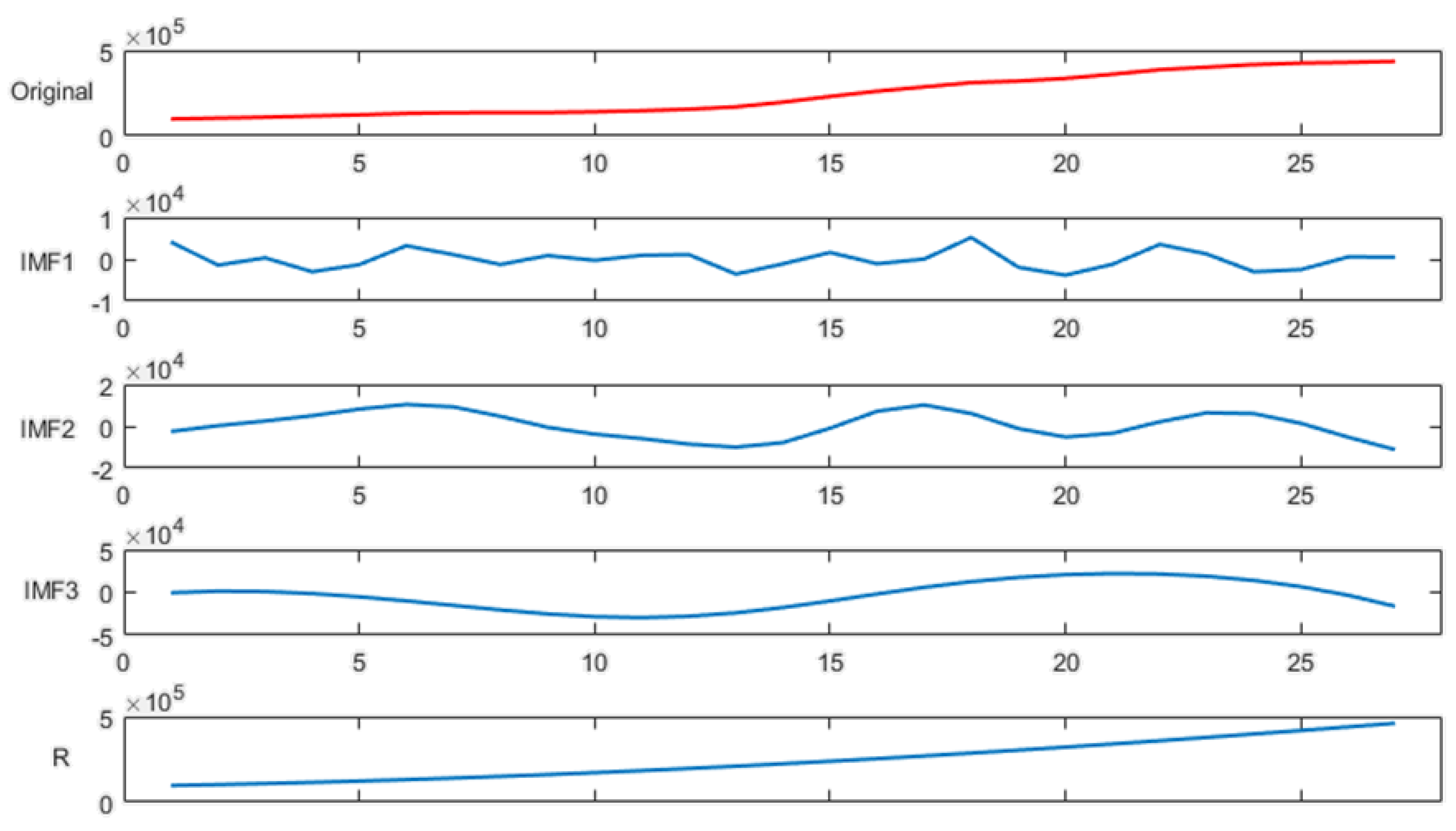
2.1. Ensemble Empirical Mode Decomposition

2.1.1. Empirical Mode Decomposition (EMD)

Empirical mode decomposition (EMD) is a new adaptive signal time frequency processing method, proposed by Huang in 1998 [38], that is especially suitable for the analysis and processing of nonlinear nonstationary signals. The method is considered to be a significant breakthrough in the linear and steady-state spectrum analysis based on the Fourier transform. The complex signal is decomposed into a finite number of Intrinsic Mode Functions (IMFs) by Empirical Mode Decomposition, and the intrinsic mode functions show the intrinsic vibrational form of the signal. The IMF components must meet the following two conditions:

(1)

The maximum difference between the number of extremes and the number of zero points is one;

(2)

The upper envelope and the lower envelope should be symmetrical.

For the signal $X\left(t\right)$, the calculation flow of EMD is as follows:

(1)

Determine all maxima and minima of signal $X\left(t\right)$;

(2)

According to the maximum and minimum of signal, construct the upper envelope $f_a\left(t\right)$ and lower envelope $f_b\left(t\right)$ of $X\left(t\right)$ using three spline interpolation method;

(3)

Find the local average of the signal, $f_m(t)=(f_a(t)+f_b(t))/2$;

(4)

Calculate the difference between $X\left(t\right)$ and $f_m(t)$, $E(t)=X(t)-f_m(t)$;

(5)

Determine whether $E(t)$ satisfies the conditions of IMF, and if the conditions are satisfied, the first IMF component can be obtained; otherwise, repeat the above steps until the signal meets the IMF conditions.

(6)

Define $r(t)=X(t)-im{f}_1(t)$, and determine whether $r(t)$ needs to be decomposed. If so, repeat the above steps by replacing $X(t)$ with $r(t)$, otherwise end the decomposition.

After all these steps, the process of EMD for the signal $X(t)$ can be ended and the signal $X(t)$ is decomposed into the sum of a number of IMF components $im{f}_i(t)$ and the remaining components $r(t)$, that is $X(t)={\displaystyle \sum _{i=1}^{n}im{f}_i(t)+r(t)}$.

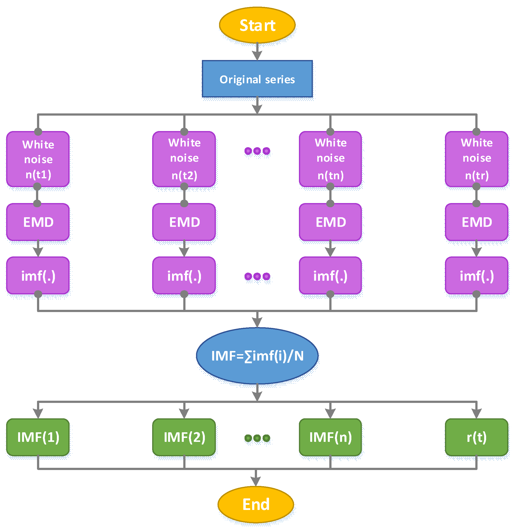
2.1.2. Ensemble Empirical Mode Decomposition (EEMD)

Modal aliasing refers to the condition that one intrinsic mode function contains the characteristic time scale with great difference, or the similar characteristic time scales are distributed in different intrinsic mode functions, which causes two adjacent intrinsic mode functions’ waveforms to be mixed and unrecognizable. Empirical Mode Decomposition may introduce the modal aliasing problem. To solve this problem, EEMD was proposed by Huang and Wu [39]. Based on the traditional EMD, the Gaussian white noise is introduced to eliminate the intermittent phenomenon in the original signal to solve the modal aliasing problem by eliminating the intermittence of the original signal using the statistical characteristics of the uniform distribution of white noise. The principle of EEMD is as follows: when additional white noise is averagely distributed in time frequency space, the time frequency space is composed of different scales segmented by filter banks.

The detailed steps of EEMD are as follows:

(1)

Add random Gaussian white noise sequence to the signal

$$X_m(t)=X(t)+k·n_m(t),$$

(1)

where $k$ is the amplitude factor of added white noise; $n_m(t)$ is the white noise sequence.

(2)

Decompose the signal into a group of intrinsic mode functions using Empirical Mode Decomposition with white noise;

(3)

Add a different white noise sequence each time, and then, repeat the steps of (1) and (2);

(4)

Calculate the mean value of decomposed IMFs, and take the average value of each IMF obtained by decomposition as the final result.

$${\overline{c}}_i=\frac{1}{N}{\displaystyle \sum _{m=1}^N{c}_{i,m}},$$

(2)

where $N$ is the integration number using EMD; $c_{i,m}$ is the $i$th IMF in the $m$th decomposition.

The process of EEMD is shown in Figure 1.

2.2. Least Squares Support Vector Machine (LSSVM)

Least Squares Support Vector Machine is an improved technique for Support Vector Machine (SVM) proposed by Suykens et al. [40] that transforms the nonlinear problem into the linear estimation problem in high-dimensional feature space through least squares value functions and equality constraints to improve the computation speed and generalization ability [16,17,18].

Supposing that the training set is $(x_i,y_i),i=1,2,\cdots ,N$, where $N$ is the total number of training samples, $x_i\in R^m$ are input samples and $y_i$ are output samples, the linear function of LSSVM in high-dimensional feature space is:

$$f(X)={\omega }^T\phi (X)+b,$$

(3)

where $\omega$ is the weight vector; $b$ is the bias constant. Considering the complexity of the function and the error of fitting in the regression problem, it can be expressed as an equality constraint optimization problem:

$$\begin{array}{l}\underset{\omega ,b,e}{\min }J(\omega ,e)=\frac{1}{2}{\omega }^T\omega +\frac{\xi }{2}{\displaystyle \sum _{i=1}^N{e}_i^2}\\ s.t.y_i={\omega }^T\phi (X)+b+e_i,i=1,2,\cdots ,N\end{array}.$$

(4)

Setting ${\alpha }_i$ as the Lagrange multipliers, through establishing Lagrange equation, Equation (4) can be transformed into unconstrained optimization problem, as shown in Equation (5):

$$L(\omega ,b,e,\alpha )=J(\omega ,e)-{\displaystyle \sum _{i=1}^N{\alpha }_i({\omega }^T\phi (x_i)+b+e_i-y_i)}.$$

(5)

According to the Karush–Kuhn–Tucker condition of non-linear optimal programming, the parameters ${\alpha }_i$ and $b$ are obtained, and substituted them into Equation (3) to get:

$$f(X)={\displaystyle \sum _{i=1}^N{\alpha }_i\phi {(x_i)}^T\phi (x_j)}+b.$$

(6)

For LSSVM, the commonly used kernel functions include linear kernel function, polynomial kernel function, Sigmoid kernel functions, and RBF (Radial Basis Function) kernel function. Linear kernel function is a special case of RBF kernel function, and compared with polynomial kernel function and Sigmoid kernel function, RBF kernel function has fewer parameters to be determined. As long as the value of kernel parameters is determined, the performance of kernel function can be played at the minimum cost. So, Radial Basis Function (RBF) is selected as the kernel function of LSSVM to achieve the prediction function of LSSVM in this article. The Radial Basis Function is a scalar function along the radial symmetry. Because the function is similar to the Gaussian distribution, it is also called a Gaussian kernel function:

$$f(X)={\displaystyle \sum _{i=1}^N{\alpha }_i\exp \left(\frac{-{\Vert x_i-x_j\Vert }^2}{2{\sigma }^2}\right)}+b.$$

(7)

2.3. Improved Shuffled Frog Leaping Algorithm

2.3.1. Shuffled Frog Leaping Algorithm (SFLA)

Shuffled Frog Leaping Algorithm was first proposed by Eusuff and Lansey in 2003. As a novel intelligent optimization technique, SFLA combines the advantages of a Memetic Algorithm and Particle Swarm Optimization. The SFLA has the key characteristics of a simple concept, fewer parameters to adjust, fast computation speed, and strong global searching ability [32,33,34].

For a D-dimensional target search space, the initial frog population is generated randomly, and the entire population consists of $F$ frogs. Then, the population is divided into $S$ sub-populations and each sub-population contains $n$ frogs, obviously, $F=S\times n$. The frogs are sorted according to the fitness. The classification of frogs is carried out according to the following principles:

(1)

Arranging the first frog in the first sub-population, the second frog in the second sub-population, the $j$th frog in the $j$th sub-population, and the $j+1$th frog in the $j+1$th sub-population, until all the frogs have been arranged into their sub-populations.

(2)

For each sub-population, fitness values of individuals are calculated. The frog with the best fitness is set as $X_b$; The frog with the worst fitness is set as $X_w$; The frogs with optimal fitness in the whole population is set as $X_g$.

(3)

During each evolution of the sub-population, local search of $X_w$ is carried out to update the sub-population. The update strategy is as follows:

$$D_i=rand()*(X_{bi}-X_{wi})$$

(8)

$$X_w^{\prime }=X_w+D_i(-D_{\max }\le D_i\le D_{\max })$$

(9)

where $rand()$ is a random value distributing between [0, 1]; $D_{\max }$ is the largest step of frog.

(4)

If the fitness value of updated frog $X_w^{\prime }$ is better than that of the original frog $X_w$, replace $X_w$ with $X_w^{\prime }$. Otherwise, replace $X_b$ with $X_g$. If the new solution obtained is still worse than the original frog $X_w$, take a randomly generated new position to replace the original frog $X_w$. Continue to repeat the above process until local search ends.

(5)

Re-divide the population and start local search again. Repeat the above steps until the algorithm meets the end condition.

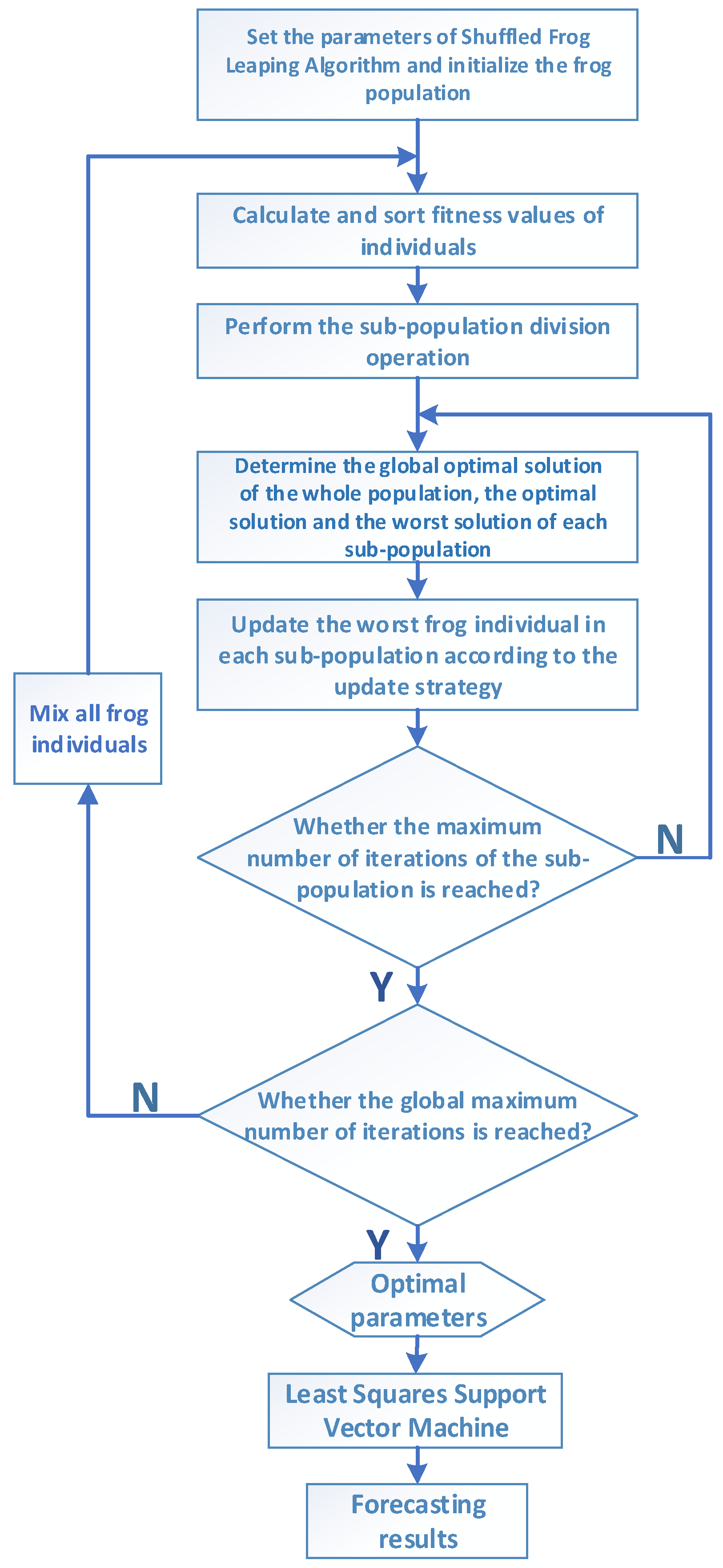
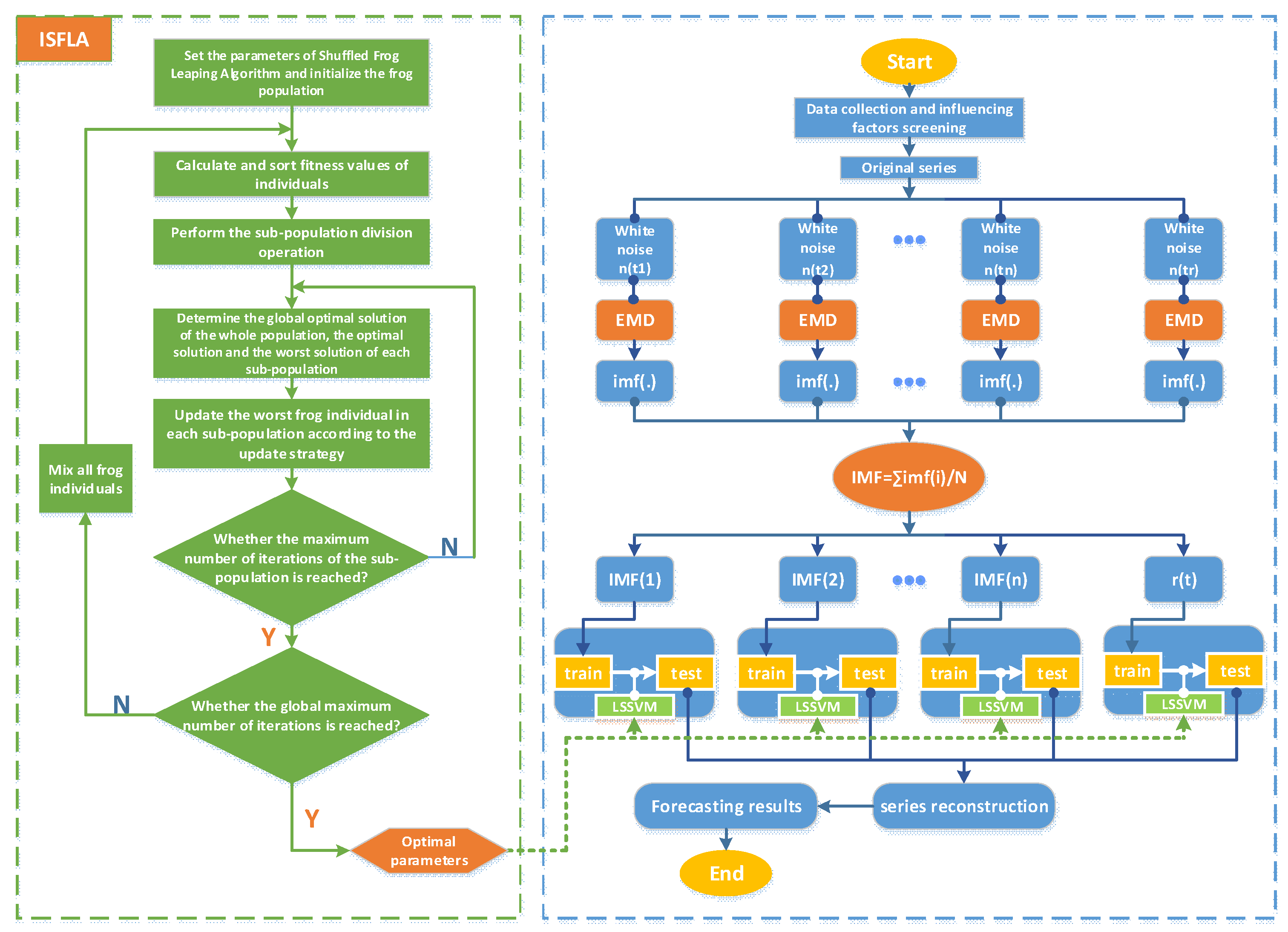
2.3.2. Improved Shuffled Frog Leaping Algorithm (ISFLA)

In traditional SFLA, the characteristics of frog individuals to be updated have a constant influence on the update individuals, which not only leads to convergence rate decline, but also easily causes it to trap into a local optimum. Therefore, for improving the searching efficiency, in this article, we introduce nonlinear decreasing inertia weight to improve the traditional SFLA algorithm to avoid local optimum solution.

After introducing nonlinear decreasing inertia weight, the update strategy is as shown in Equation (10):

$$X_w^{\prime }=\omega X_w+D_i(-D_{\max }\le D_i\le D_{\max }).$$

(10)

The inertia weight $\omega$ reflects the frog’s movement tendency. The traditional inertia weight value decreases linearly with the increase in population iteration number, which is simple and direct, but difficult to reflect in the complex local search process; in addition, it is easy to trap into a local optimum. Therefore, in this paper, we adopt nonlinear decreasing inertia weight:

$$\omega ={({\omega }_{\max }-{\omega }_{\min })}^{\sqrt{t/k}}+{\omega }_{\min }^2,$$

(11)

where ${\omega }_{\max }$ is the maximum inertia weight; ${\omega }_{\min }$ is the minimum inertia weight; $t$ is the product of the iteration number of current sub-population and number of iterations of the whole population; $k$ is number of iterations of the sub-population. The above descending process makes the value of $\omega$ decrease from large to small, which reduces the probability of the algorithm falling into the local optimum to a certain extent.

2.4. Least Squares Support Vector Machine Optimized by Improved Shuffled Frog Leaping Algorithm

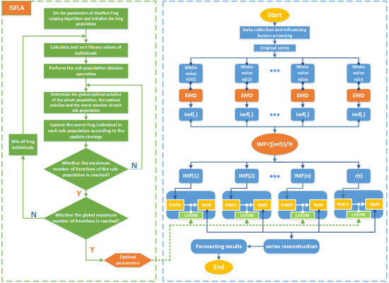
Using the Least Squares Support Vector Machine with RBF kernel function to forecast energy consumption, two parameters that will directly affect the performance of the model including the parameter of regularization and the width of the radial basis function should be determined. In this article, Improved Shuffled Frog Leaping Algorithm is used to optimize the parameters of Least Squares Support Vector Machine. The flow is as follows:

(1)

Set the Shuffled Frog Leaping Algorithm parameters and initialize the frog population;

(2)

Calculate the frog individuals’ fitness values and sort them;

(3)

Divide sub-populations and determine the global optimal solution of the whole population, the optimal solution and the worst solution of each sub-population;

(4)

Search and update the worst local frog individuals in each sub-population until the local search ends;

(5)

Mix the updated subgroups;

(6)

Determine whether the maximum iterative number is reached. If so, stop optimization and output the optimal solution. Otherwise, turn to Step (2);

(7)

Assign the optimized parameters to Least Squares Support Vector Machine for constructing the forecasting model.

The flowchart of Least Squares Support Vector Machine Optimized by Improved Shuffled Frog Leaping Algorithm (ISFLA-LSSVM) is shown in Figure 2.

2.5. The Forecasting Model Based on Ensemble Empirical Mode Decomposition and Least Squares Support Vector Machine Optimized by Improved Shuffled Frog Leaping Algorithm (EEMD-ISFLA-LSSVM)

The forecasting accuracy of energy consumption is influenced by various factors. For improving the accuracy, in this article, on the basis of considering the energy consumption influencing factors of population, GDP, industrial structure (the proportion of the second industry added value), energy consumption structure, energy intensity, carbon emission intensity and total imports and exports, the EEMD-ISFLA-LSSVM model for energy consumption forecasting is proposed. The forecasting process is as follows:

(1) Data collection and influencing factors screening.

Collect the sample data, including historical energy consumption data, population, GDP, industrial structure (the proportion of the second industry added value), energy consumption structure, energy intensity, carbon emission intensity and total imports and exports, and do the dimensionless processing for the data. Then, the grey relational degrees between each influencing factor and the energy consumption are calculated, and the factors for model input are screened according to the ranking of grey relational degree.

(2) Sequence noise reduction based on Ensemble Empirical Mode Decomposition.

Do Ensemble Empirical Mode Decomposition for energy consumption sequence to obtain multiple IMF components.

(3) Energy consumption forecasting based on Least Squares Support Vector Machine Optimized by Improved Shuffled Frog Leaping Algorithm.

On the basis of considering the influencing factors of energy consumption prediction, the ISFLA-LSSVM model is used to forecast the IMF components that are obtained through EEMD, and the prediction results are reconstructed for obtaining the final energy consumption forecasting result. First, set the Shuffled Frog Leaping Algorithm parameters and initialize the frog population. Calculate the frog individuals’ fitness values and sort them. Then, divide sub-populations and determine the global optimal solution of the whole population, the optimal solution and the worst solution of each sub-population. Next, search and update the worst local frog individuals in each sub-population until the local search ends, and mix the updated subgroups. Repeat the above process until the number of iterations is reached. Finally, assign the optimized parameters to Least Squares Support Vector Machine, and the forecasting model is established to predict the IMF components.

The forecasting process based on the EEMD-ISFLA-LSSVM model is shown in Figure 3.

3. Empirical Analysis

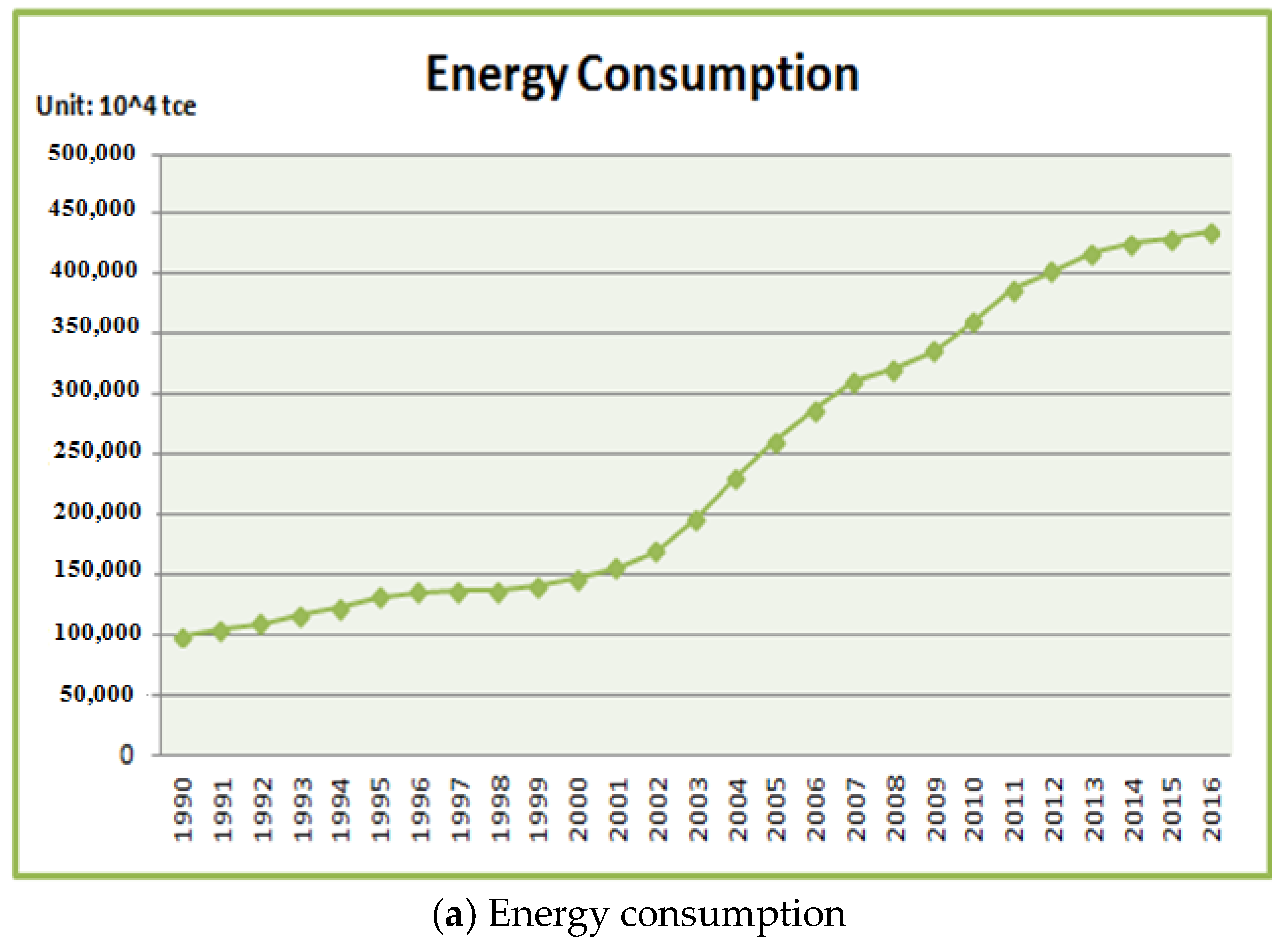
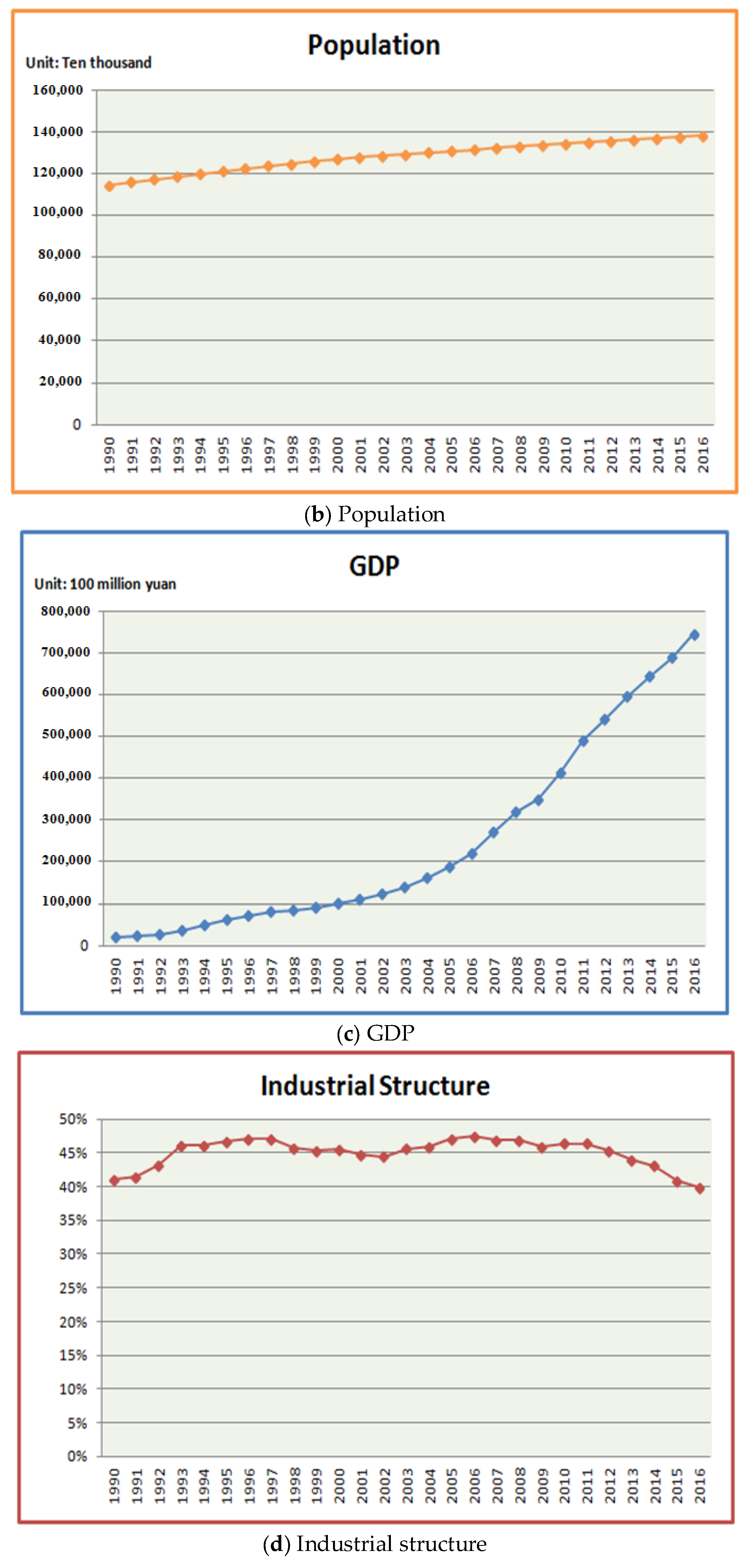
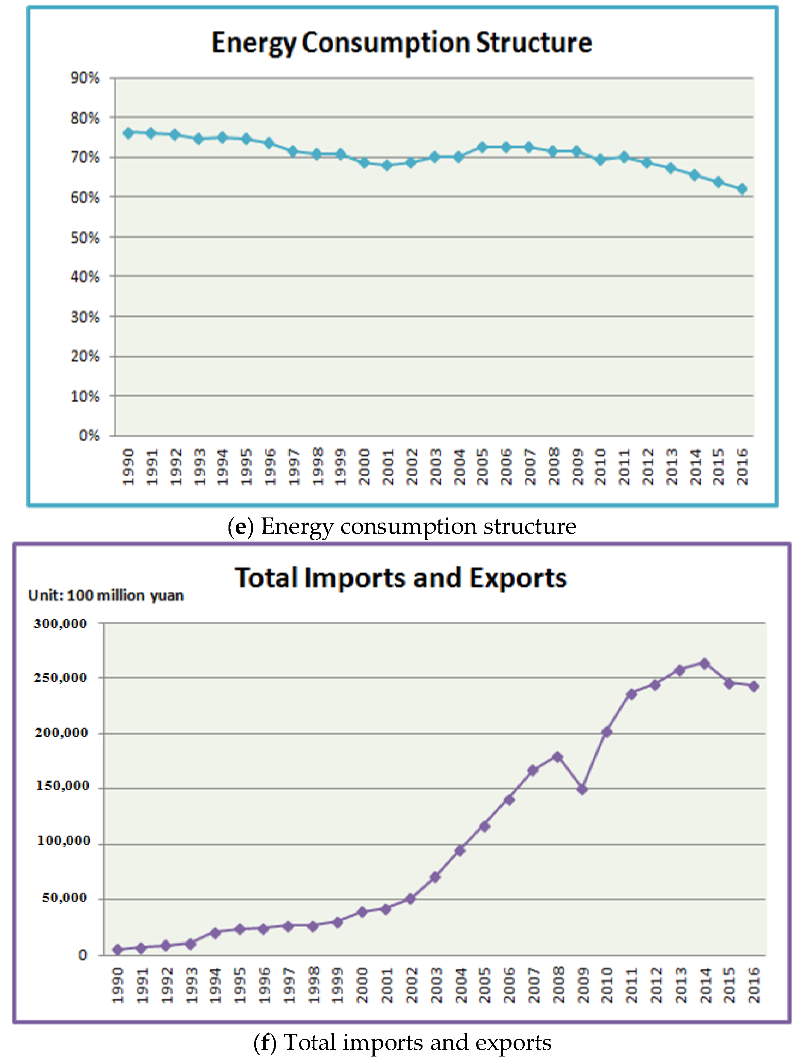
3.1. Influencing Factors Screening for Model Input

In this article, the data of the population, GDP, industrial structure, energy consumption structure, energy intensity, carbon emissions intensity, total imports and exports and other energy consumption influencing factors from 1990 to 2016 in China are collected. (The data source is the World Bank Database and China Statistical Yearbook.)

In order to determine the prediction model input, we use the grey relational degree to screen the influencing factors of energy consumption for realizing the feature reduction. The results of the calculation for grey relational degrees between the various influencing factors and the energy consumption are as follows:

In the light of

Table 1. The calculation results of the grey relational degrees for influencing factors.

Influencing Factor	Grey Relational Degree
population	0.7781
GDP	0.8088
industrial structure	0.7624
energy consumption structure	0.7545
energy intensity	0.6568
carbon emissions intensity	0.6530
total imports and exports	0.8181

, we select the five factors whose grey relational degree is greater than 0.7 as the energy consumption forecasting model input. They are population, GDP, industrial structure, energy consumption structure and total imports and exports. The model output is the energy consumption.

The data of the energy consumption, population, GDP, industrial structure, energy consumption structure and total imports and exports from 1990 to 2016 in China are shown in Figure 4.

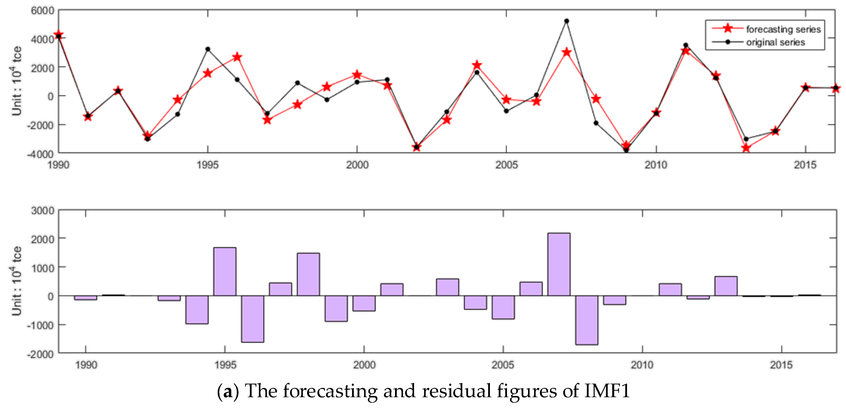
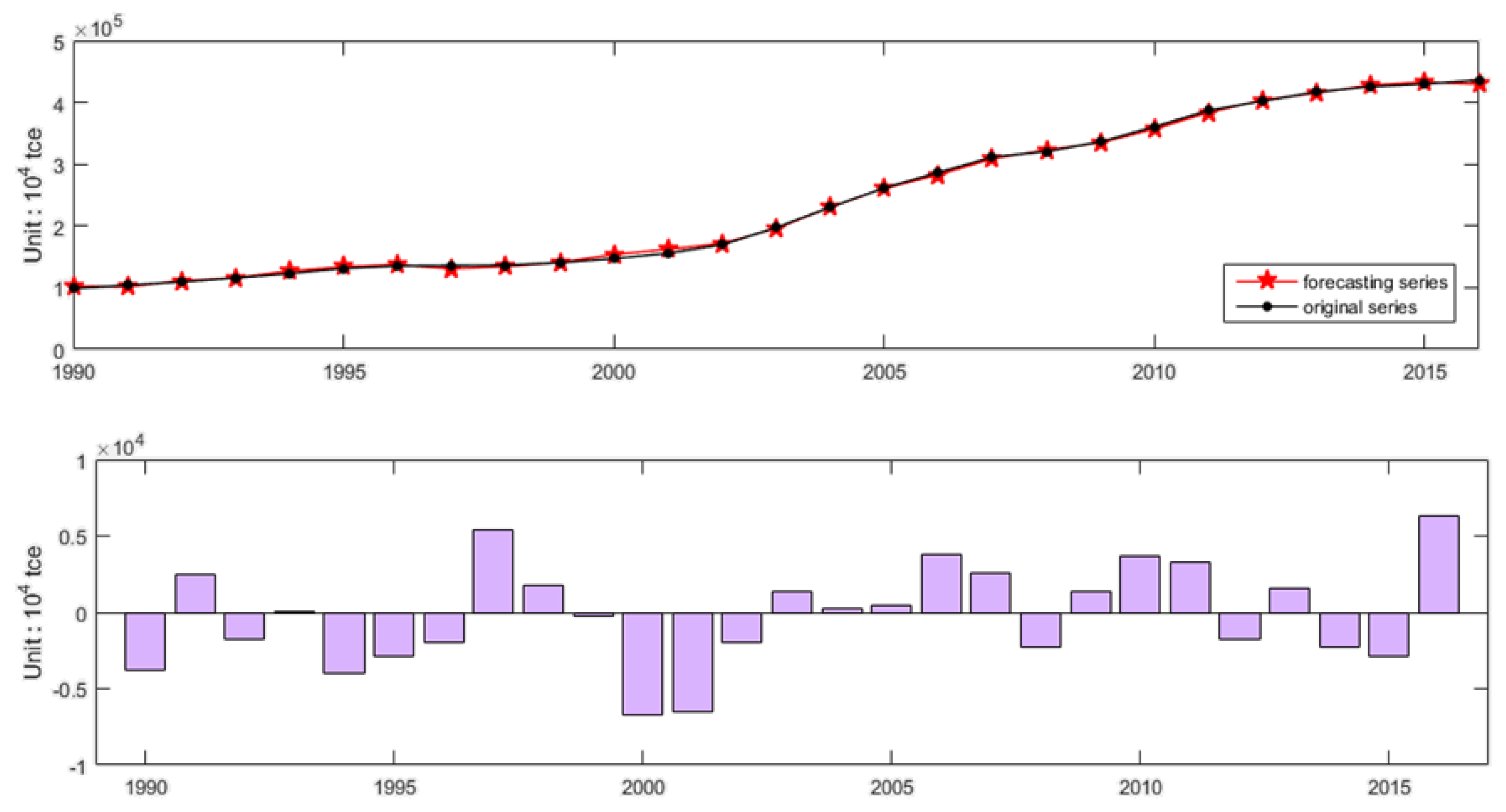
3.2. Forecasting of Energy Consumption in China Based on EEMD-ISFLA-LSSVM Model

In order to predict energy consumption in China accurately, we first take the ensemble empirical mode decomposition of the original energy consumption sequence to achieve data de-noising. By EEMD, three IMFs and one residual signal are obtained, which are shown in Figure 5.

The data from 1990 to 2009 are taken as the training set, and the test set is the data from 2010 to 2016. The ISFLA-LSSVM model is adopted to predict the IMF components and the residual signal obtained above. The algorithm parameters settings are as follows: the frog population is 500. The sub-population is 50. The sub-population search number is 10. The regularization parameter search range of LSSVM is [0.1, 150], and the RBF kernel parameter is [0.01, 30]. The maximum number of iterations is 150. The prediction results and the residuals are shown in Figure 6.

The prediction results of the IMFs and the residual signal are reconstructed. Then the final prediction result of energy consumption are obtained, which are shown in Figure 7.

The calculation equation of the relative error $RE$ is shown in Equation (12):

$$RE=\frac{\left|{\widehat{y}}_i-y_i\right|}{y_i}\times 100\%.$$

(12)

The relative errors of each prediction point are shown in

Table 2. The relative error.

Year	Actual Value (104 tce)	Forecasting Value (104 tce)	RE (%)
1990	98,703	102,498	3.85
1991	103,783	101,262	2.43
1992	109,170	110,988	1.67
1993	115,993	115,923	0.06
1994	122,737	126,733	3.26
1995	131,176	134,031	2.18
1996	135,192	137,139	1.44
1997	135,909	130,536	3.95
1998	136,184	134,441	1.28
1999	140,569	140,805	0.17
2000	146,964	153,695	4.58
2001	155,547	162,075	4.20
2002	169,577	171,559	1.17
2003	197,083	195,744	0.68
2004	230,281	230,056	0.10
2005	261,369	260,912	0.17
2006	286,467	282,653	1.33
2007	311,442	308,834	0.84
2008	320,611	322,859	0.70
2009	336,126	334,721	0.42
2010	360,648	356,996	1.01
2011	387,043	383,739	0.85
2012	402,138	403,889	0.44
2013	416,913	415,380	0.37
2014	425,806	428,055	0.53
2015	429,905	432,790	0.67
2016	436,000	429,665	1.45

.

According to Figure 7 and Table 2, using the EEMD-ISFLA-LSSVM model to forecast the energy consumption, the fitting degree between the prediction curve and the actual curve is very good, and the prediction effect is significant. The relative errors of all prediction points are not more than 5%.

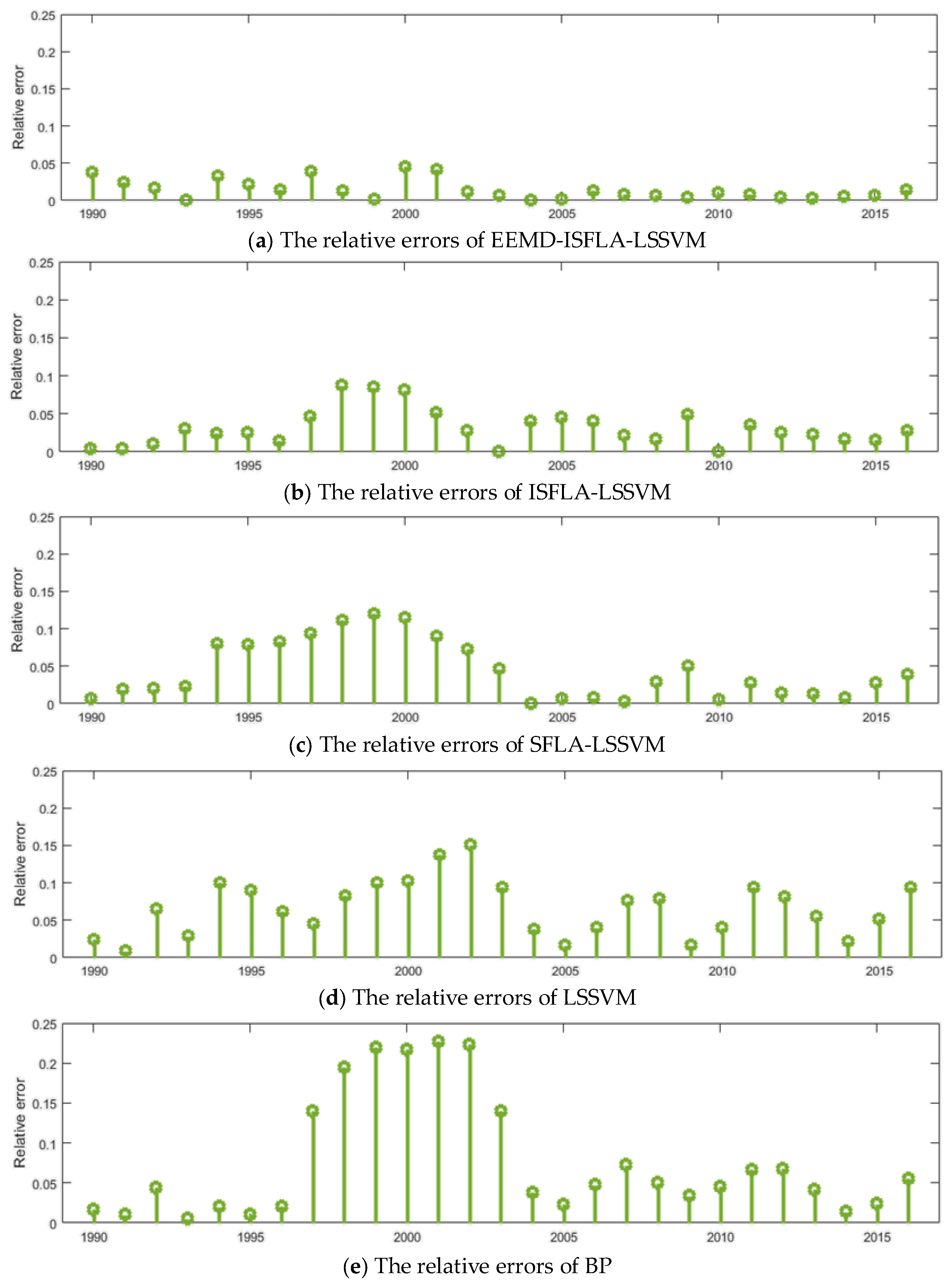
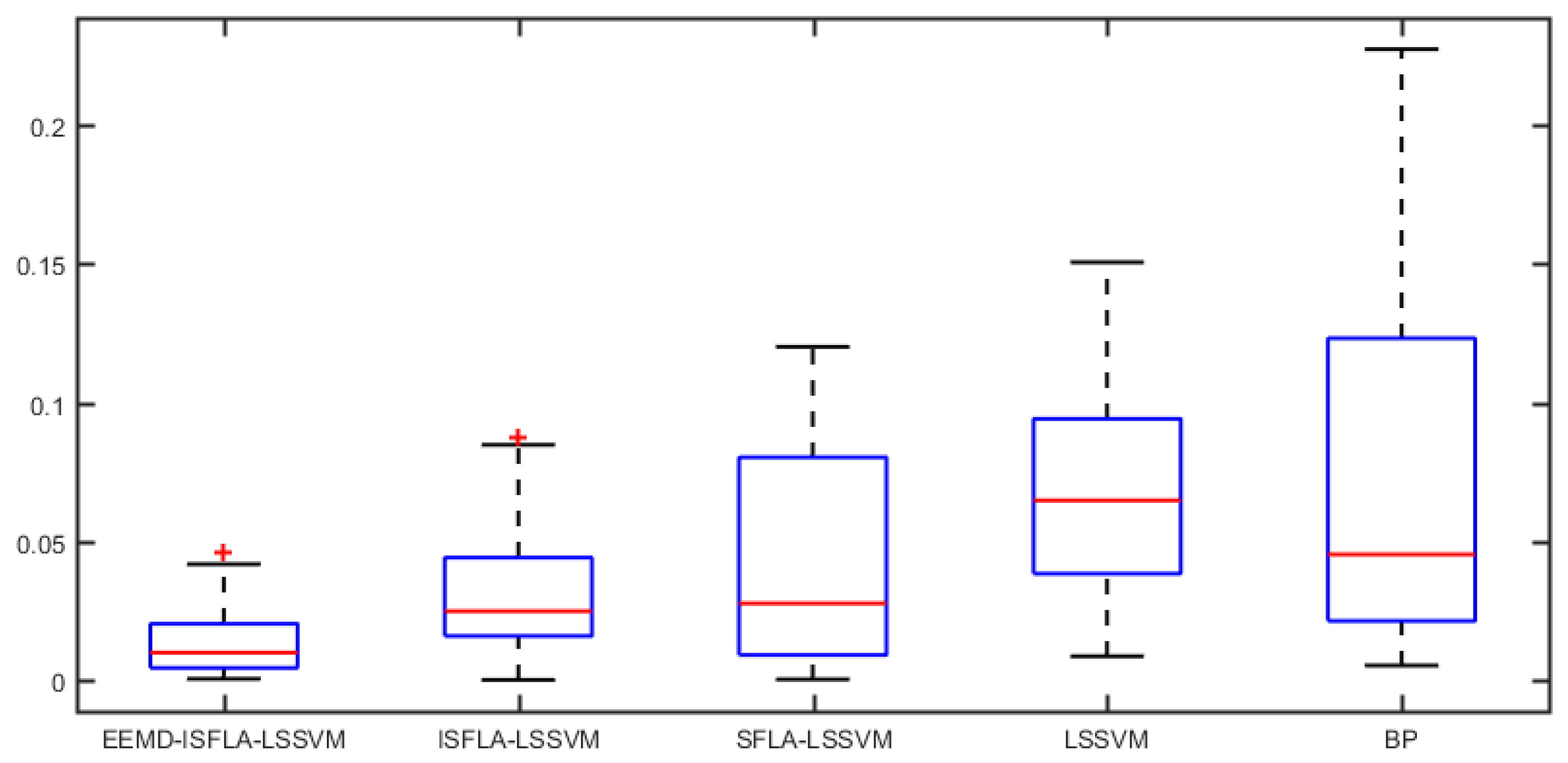
3.3. Model Comparison and Error Analysis

In fact, EEMD-ISFLA-LSSVM is a complex combination model, which comes from the improvement and combination of a variety of single models. The EEMD-ISFLA-LSSVM model has evolved from the models of BP neural network, LSSVM, SFLA-LSSVM and ISFLA-LSSVM, which shows the thinking process for proposing the model. For proving the validity and superiority of the EEMD-ISFLA-LSSVM model further, four models of ISFLA-LSSVM, SFLA-LSSVM, LSSVM, and BP neural network are selected to make a comparison with the EEMD-ISFLA-LSSVM model by the same sample, which can prove that the combination model is obviously superior to single algorithm and introducing the noise reduction method of EEMD is helpful for improving the prediction accuracy. The parameter settings of the ISFLA-LSSVM, SFLA-LSSVM, and LSSVM models are the same as those of the EEMD-ISFLA-LSSVM model. The parameter settings of the BP neural network are as follows: the initial weight is a random number between (−1, 1); the activation functions between the input layer and the hidden layer, the hidden layer and the output layer are both Sigmoid functions; the hidden layer function is a tansig transfer function; the output layer function is a logsig transfer function; the learning rate is 0.1; the momentum factor is 0.8; the network global error is 0.001; the maximum number of training is 500; the number of hidden layer nodes is 11.

The comparison results, relative error, and boxplot of relative error are shown in Figure 8, Figure 9 and Figure 10.

Figure 8 shows the fitting degree between the energy consumption curve forecasted by different models and the actual curve of energy consumption. The forecasting curve of the EEMD-ISFLA-LSSVM model fits the actual curve best. Figure 9 shows the relative errors of each model for energy consumption forecasting. The boxplot in Figure 10 shows the relative errors’ minimum, first quartile, the median, third quartile and the maximum in each model. From Figure 9 and Figure 10, it can be seen that EEMD-ISFLA-LSSVM model has the minimum relative error, followed by ISFLA-LSSVM model, SFLA-LSSVM model, LSSVM model, and BP has the maximum relative error.

For evaluating the forecasting effect of each model more objectively, $MAPE$ (mean absolute percentage error), $RMSE$ (root mean square error) and $MAE$ (mean absolute error) are applied to compare the prediction accuracy. The calculation equations are shown as follows:

$$MAPE=\frac{1}{n}{\displaystyle \sum _{i=1}^n\left|\frac{{\widehat{y}}_i-y_i}{y_i}\right|}$$

(13)

$$RMSE=\sqrt{\frac{1}{n}{\displaystyle \sum _{i=1}^n{({\widehat{y}}_i-y_i)}^2}}$$

(14)

$$MAE=\frac{1}{n}{\displaystyle \sum _{i=1}^n\left|{\widehat{y}}_i-y_i\right|}.$$

(15)

The calculation results of $MAPE$, $RMSE$ and $MAE$ for different models are shown below.

From

Table 3. The calculation results.

Model	MAPE (%)	RMSE (107 tce)	MAE (107 tce)
EEMD-ISFLA-LSSVM	1.47	3.27	2.72
ISFLA-LSSVM	3.16	8.46	7.04
SFLA-LSSVM	4.42	10.08	8.28
LSSVM	6.66	18.62	15.45
BP	7.68	19.68	15.94

, it can be concluded that the $MAPE$, $RMSE$ and $MAE$ of the EEMD-ISFLA-LSSVM model are the smallest of all the models, reaching 1.47%, 3.27, and 2.72, respectively. Next is the ISFLA-LSSVM model: the $MAPE$, $RMSE$ and $MAE$ are 3.16%, 8.46, and 7.04, respectively. The $MAPE$, $RMSE$ and $MAE$ of the BP model are the largest, reaching 7.68%, 19.68, and 15.94, respectively. Moreover, SFLA-LSSVM model has better forecasting ability than LSSVM. It can be seen that the evaluation results of the three indexes for the five models tend to be consistent. Ranking the prediction accuracy of five models based on different indexes, we can get the same ranking result as follows: EEMD-ISFLA-LSSVM > ISFLA-LSSVM > SFLA-LSSVM > LSSVM > BP. According to the ranking results, as a complex combination model for energy consumption prediction, EEMD-ISFLA-LSSVM can combine the advantages of different algorithms, whose forecasting effect is obviously superior to that of a single algorithm, such as LSSVM and BP neural network. Taking the signal decomposition of the original energy consumption sequence can effectively reduce the sequence noise and achieve a better prediction in light of the prediction accuracy comparison between EEMD-ISFLA-LSSVM and ISFLA-LSSVM. It can be seen that the improved optimization algorithm has the advantage over the original optimization algorithm in parameter optimization based on the prediction accuracy comparison between ISFLA-LSSVM and SFLA-LSSVM. To sum up, we can conclude that the prediction accuracy of EEMD-ISFLA-LSSVM model is obviously higher than that of other models, which makes it effective and practical for energy consumption forecasting.

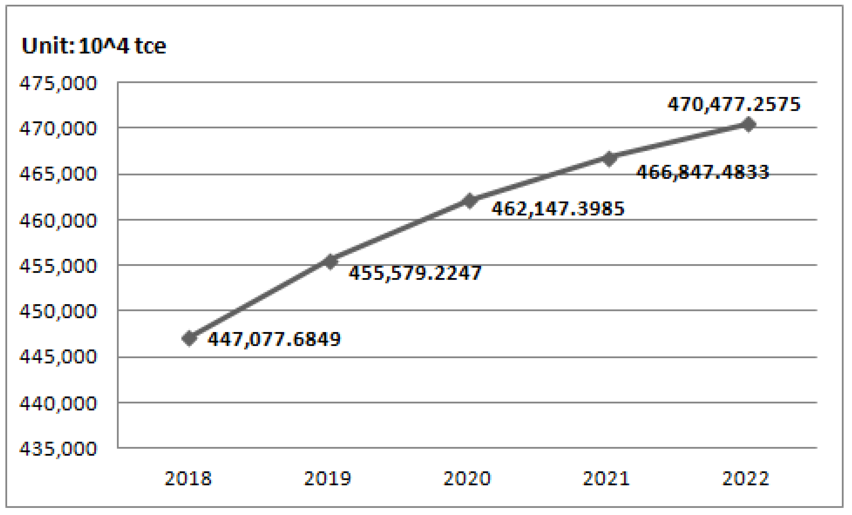
3.4. Forecasting of Energy Consumption in China Based on the EEMD-ISFLA-LSSVM Model

On the basis of the collected historical data from 1990 to 2016 in China, grey model is used to forecast the influencing factors for China’s energy consumption from 2018 to 2022. The predicted data of the influencing factors are used as the EEMD-ISFLA-LSSVM model input to forecast the energy consumption from 2018 to 2022 in China. The specific forecasting results are shown in Figure 11.

As seen in Figure 11, China’s energy consumption from 2018 to 2022 has a trend of significant growth. With the rapid development of China’s energy consumption, it is foreseeable that the energy consumption will continue increasing in the future.

4. Conclusions

In order to forecast the energy consumption of China accurately, considering the main driving factors of energy consumption, the novel model of EEMD-ISFLA-LSSVM is proposed in this article. The prediction accuracy of energy consumption is influenced by various factors. In this article, first considering population, GDP, industrial structure (the proportion of the second industry added value), energy consumption structure, energy intensity, carbon emissions intensity, total imports and exports and other influencing factors of energy consumption, the main driving factors of energy consumption are screened as the model input according to the sorting of grey relational degrees to realize feature dimension reduction. Then, the original energy consumption sequence of China is decomposed into multiple sub sequences by Ensemble Empirical Mode Decomposition for de-noising. Next, the ISFLA-LSSVM model is adopted to forecast each subsequence, and the prediction sequences are reconstructed to obtain the forecasting result. After that, we make an empirical analysis for energy consumption prediction, and four models (ISFLA-LSSVM, SFLA-LSSVM, LSSVM, and BP neural network) are selected to compare with the EEMD-ISFLA-LSSVM model, which proves the practicability and validity of the EEMD-ISFLA-LSSVM model for energy consumption forecasting in China. Finally, the EEMD-ISFLA-LSSVM model is adopted to forecast energy consumption in China from 2018 to 2022, and according to the forecasting results, it can be seen that China’s energy consumption from 2018 to 2022 will have a trend of significant growth.

References

1. Hsu, C.C.; Chen, C.Y. Applications of improved grey prediction model for power demand forecasting. Energy Convers. Manag. 2003, 44, 2241–2249. [Google Scholar] [CrossRef]
2. Lin, C.S.; Liou, F.M.; Huang, C.P. Grey forecasting model for CO2 emissions: A Taiwan study. Adv. Mater. Res. 2011, 88, 3816–3820. [Google Scholar] [CrossRef]
3. Lee, Y.S.; Tong, L.I. Forecasting energy consumption using a grey model improved by incorporating genetic programming. Energy Convers. Manag. 2011, 52, 147–152. [Google Scholar] [CrossRef]
4. Acaroglu, O.; Ozdemir, L.; Asbury, B. A fuzzy logic model to predict specific energy requirement for TBM performance prediction. Tunn. Undergr. Space Technol. 2008, 23, 600–608. [Google Scholar] [CrossRef]
5. Gokulachandran, J.; Mohandas, K. Application of Regression and Fuzzy Logic Method for Prediction of Tool Life. Proc. Eng. 2012, 38, 3900–3912. [Google Scholar] [CrossRef]
6. Chen, S.X.; Gooi, H.B.; Wang, M.Q. Solar radiation forecast based on fuzzy logic and neural networks. Renew. Energy 2013, 60, 195–201. [Google Scholar] [CrossRef]
7. Ismail, Z.; Yahaya, A.; Shabri, A. Forecasting Gold Prices Using Multiple Linear Regression Method. Am. J. Appl. Sci. 2009, 6, 1509–1514. [Google Scholar] [CrossRef]
8. Sehgal, V.; Tiwari, M.K.; Chatterjee, C. Wavelet Bootstrap Multiple Linear Regression Based Hybrid Modeling for Daily River Discharge Forecasting. Water Resour. Manag. 2014, 28, 2793–2811. [Google Scholar] [CrossRef]
9. Mu, H.; Dong, X.; Wang, W.; Ning, Y.; Zhou, W. Improved Gray Forecast Models for China’s Energy Consumption and CO, Emission. J. Desert Res. 2002, 22, 142–149. [Google Scholar]
10. Lau, H.C.W.; Cheng, E.N.M.; Lee, C.K.M.; Ho, C.T.S. A fuzzy logic approach to forecast energy consumption change in a manufacturing system. Expert Syst. Appl. 2008, 34, 1813–1824. [Google Scholar] [CrossRef]
11. Aranda, A.; Ferreira, G.; Mainar-Toledo, M.D.; Scarpellini, S.; Sastresa, E.L. Multiple regression models to predict the annual energy consumption in the Spanish banking sector. Energy Build. 2012, 49, 380–387. [Google Scholar] [CrossRef]
12. Yang, J.F.; Cheng, H.Z. Application of SVM to power system short-term load forecast. Electr. Power Autom. Equip. 2004, 24, 30–32. [Google Scholar]
13. Zhou, J.G.; Zhang, X.G. Projections about Chinese CO2 emissions based on rough sets and gray support vector machine. China Environ. Sci. 2013, 33, 2157–2163. [Google Scholar]
14. Shi, X.; Huang, Q.; Chang, J.; Wang, Y.; Lei, J.; Zhao, J. Optimal parameters of the SVM for temperature prediction. Proc. Int. Assoc. Hydrol. Sci. 2015, 368, 162–167. [Google Scholar] [CrossRef]
15. Hong, W.C. Electric load forecasting by support vector model. Appl. Math. Model. 2009, 33, 2444–2454. [Google Scholar] [CrossRef]
16. Li, X.; Wang, X.; Zheng, Y.H.; Li, L.X.; Zhou, L.D.; Sheng, X.K. Short-Term Wind Power Forecasting Based on Least-Square Support Vector Machine (LSSVM). Appl. Mech. Mater. 2013, 448, 1825–1828. [Google Scholar] [CrossRef]
17. De Giorgi, M.G.; Malvoni, M.; Congedo, P.M. Comparison of strategies for multi-step ahead photovoltaic power forecasting models based on hybrid group method of data handling networks and least square support vector machine. Energy 2016, 107, 360–373. [Google Scholar] [CrossRef]
18. Zhao, H.; Guo, S.; Zhao, H. Energy-Related CO2 Emissions Forecasting Using an Improved LSSVM Model Optimized by Whale Optimization Algorithm. Energies 2017, 10, 874. [Google Scholar] [CrossRef]
19. Sun, W.; He, Y.; Chang, H. Forecasting Fossil Fuel Energy Consumption for Power Generation Using QHSA-Based LSSVM Model. Energies 2015, 8, 939–959. [Google Scholar] [CrossRef]
20. Ahmad, A.S.B.; Hassan, M.Y.B.; Majid, M.S.B. Application of hybrid GMDH and Least Square Support Vector Machine in energy consumption forecasting. In Proceedings of the IEEE International Conference on Power and Energy, Kota Kinabalu, Malaysia, 2–5 December 2012. [Google Scholar]
21. Gutjahr, W.J. ACO algorithms with guaranteed convergence to the optimal solution. Inform. Process. Lett. 2002, 82, 145–153. [Google Scholar] [CrossRef]
22. Liu, H.Y.; Jiang, Z.J. Research on Failure Prediction Technology Based on Time Series Analysis and ACO-LSSVM. Comput. Mod. 2013, 1, 219–222. [Google Scholar] [CrossRef]
23. Ying, E. Network Safety Evaluation of Universities Based on Ant Colony Optimization Algorithm and Least Squares Support Vector Machine. J. Converg. Inf. Technol. 2012, 7, 419–427. [Google Scholar] [CrossRef]
24. Karaboga, D.; Basturk, B. A powerful and efficient algorithm for numerical function optimization: Artificial bee colony (ABC) algorithm. J. Glob. Optim. 2007, 39, 459–471. [Google Scholar] [CrossRef]
25. Akay, B.; Karaboga, D. A modified Artificial Bee Colony algorithm for real-parameter optimization. Inf. Sci. 2012, 192, 120–142. [Google Scholar] [CrossRef]
26. Mirjalili, S.; Saremi, S.; Mirjalili, S.M.; Coelho, L.d.S. Multi-objective grey wolf optimizer: A novel algorithm for multi-criterion optimization. Expert Syst. Appl. 2016, 47, 106–119. [Google Scholar] [CrossRef]
27. Mirjalili, S.; Mirjalili, S.M.; Lewis, A. Grey Wolf Optimizer. Adv. Eng. Softw. 2014, 69, 46–61. [Google Scholar] [CrossRef]
28. Xu, D.Y.; Ding, S. Research on improved GWO-optimized SVM-based short-term load prediction for cloud computing. Comput. Eng. Appl. 2017, 53, 68–73. [Google Scholar]
29. Long, W.; Liang, X.-M.; Long, Z.-Q.; Li, Z.-H. Parameters selection for LSSVM based on modified ant colony optimization in short-term load forecasting. J. Cent. South Univ. 2011, 42, 3408–3414. [Google Scholar]
30. Yusof, Y.; Kamaruddin, S.S.; Husni, H.; Ku-Mahamud, K.R.; Mustaffa, Z. Forecasting Model Based on LSSVM and ABC for Natural Resource Commodity. Int. J. Comput. Theory Eng. 2013, 5, 906–909. [Google Scholar] [CrossRef]
31. Mustaffa, Z.; Sulaiman, M.H.; Kahar, M.N.M. Training LSSVM with GWO for price forecasting. In Proceedings of the International Conference on Informatics, Electronics & Vision, Fukuoka, Japan, 15–18 June 2015. [Google Scholar]
32. Pan, Q.K.; Wang, L.; Gao, L.; Li, J. An effective shuffled frog-leaping algorithm for lot-streaming flow shop scheduling problem. Int. J. Adv. Manuf. Technol. 2011, 52, 699–713. [Google Scholar] [CrossRef]
33. Eusuff, M.; Lansey, K.; Pasha, F. Shuffled frog-leaping algorithm: A memetic meta-heuristic for discrete optimization. Eng. Optim. 2006, 38, 129–154. [Google Scholar] [CrossRef]
34. Zhao, Z.; Xu, Q.; Jia, M. Improved shuffled frog leaping algorithm-based BP neural network and its application in bearing early fault diagnosis. Neural Comput. Appl. 2016, 27, 375–385. [Google Scholar] [CrossRef]
35. Wang, T.; Zhang, M.; Yu, Q.; Zhang, H. Comparing the application of EMD and EEMD on time-frequency analysis of seimic signal. J. Appl. Geophys. 2012, 83, 29–34. [Google Scholar] [CrossRef]
36. Jiang, X.; Zhang, L.; Chen, X. Short-term forecasting of high-speed rail demand: A hybrid approach combining ensemble empirical mode decomposition and gray support vector machine with real-world applications in China. Transp. Res. C Emerg. Technol. 2014, 44, 110–127. [Google Scholar] [CrossRef]
37. Liu, Z.; Sun, W.; Zeng, J. A new short-term load forecasting method of power system based on EEMD and SS-PSO. Neural Comput. Appl. 2014, 24, 973–983. [Google Scholar] [CrossRef]
38. Huang, N.E.; Shen, Z.; Long, S.R.; Wu, M.C.; Shih, H.H.; Zheng, Q.; Yen, N.; Tung, C.C.; Liu, H.H. The Empirical Mode Decomposition and the Hilbert Spectrum for Nonlinear and Non-Stationary Time Series Analysis. Proc. R. Soc. A Math. Phys. Eng. Sci. 1998, 454, 903–995. [Google Scholar] [CrossRef]
39. Wu, Z.H.; Huang, N.E.; Chen, X. The Multi-Dimensional Ensemble Empirical Mode Decomposition Method. Adv. Adapt. Data Anal. 2009, 1, 339–372. [Google Scholar] [CrossRef]
40. Suykens, J.A.K.; Vandewalle, J. Least Squares Support Vector Machine Classifiers. Neural Process. Lett. 1999, 9, 293–300. [Google Scholar] [CrossRef]
Figure 1. The process of Ensemble Empirical Mode Decomposition (EEMD). EMD, Empirical Mode Decomposition; IMF, Intrinsic Mode Function.
Applsci 08 00678 g001
Figure 2. The flowchart of Improved Shuffled Frog Leaping Algorithm (ISFLA-LSSVM).
Applsci 08 00678 g002
Figure 3. The flowchart of EEMD-ISFLA-LSSVM.
Applsci 08 00678 g003
Figure 4. The sample data.
Applsci 08 00678 g004aApplsci 08 00678 g004bApplsci 08 00678 g004c
Figure 5. The IMFs of EEMD.
Applsci 08 00678 g005
Figure 6. The forecasting results of IMFs.
Applsci 08 00678 g006aApplsci 08 00678 g006b
Figure 7. The prediction and residual figures of the final prediction result.
Applsci 08 00678 g007
Figure 8. Comparison of forecasting results.
Applsci 08 00678 g008
Figure 9. The relative errors of five models: (a) EEMD-ISFLA-LSSVM; (b) ISFLA-LSSVM; (c) SFLA-LSSVM; (d) LSSVM; (e) BP.
Applsci 08 00678 g009
Figure 10. The boxplot for five models.
Applsci 08 00678 g010
Figure 11. The forecasting results of energy consumption from 2018 to 2022 in China.
Applsci 08 00678 g011