Dynamic Response of a Long-Span Concrete-Filled Steel Tube Tied Arch Bridge and the Riding Comfort of Monorail Trains


Abstract
1. Introduction
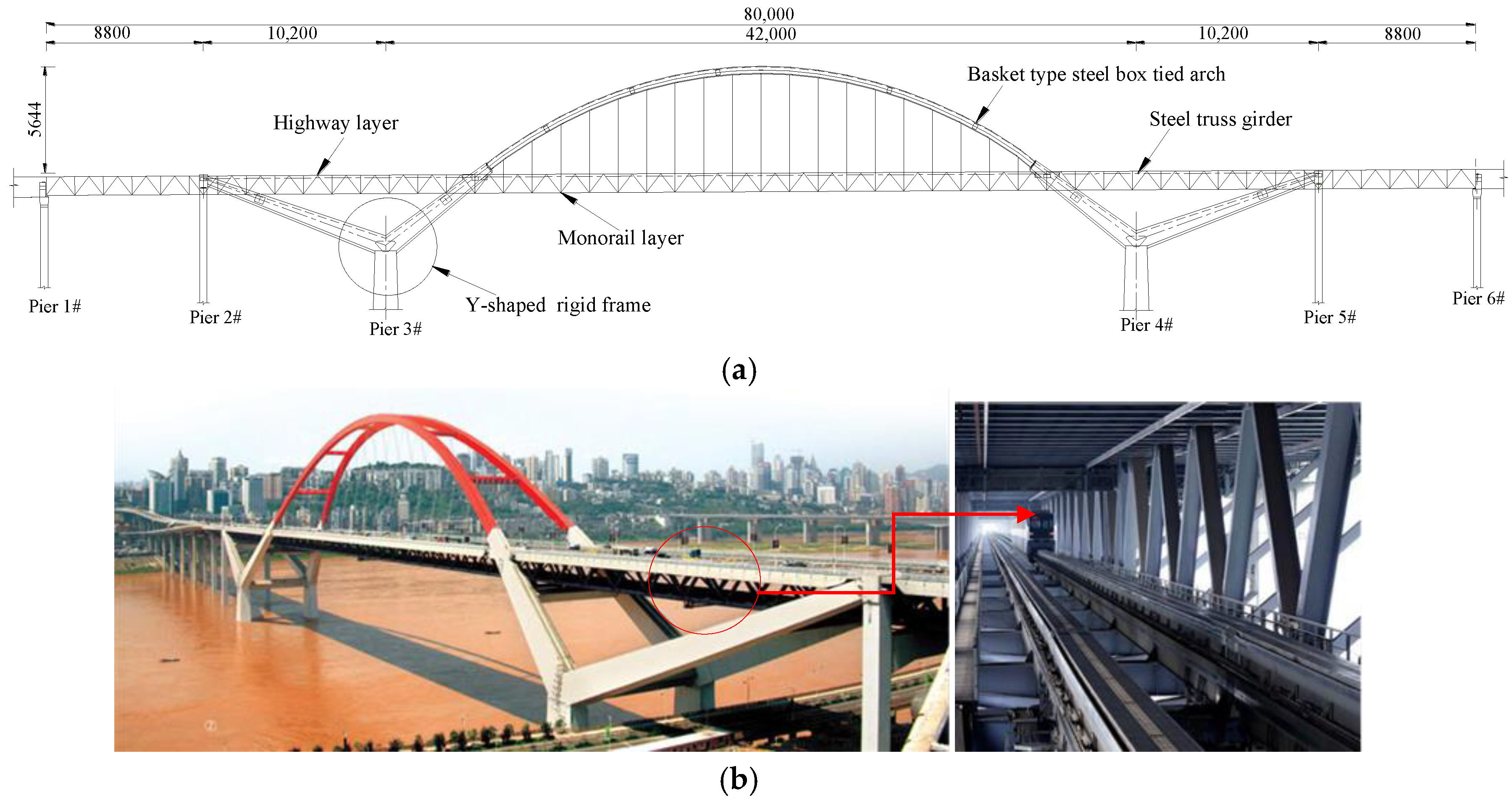
2. Bridge Description
3. Coupled Monorail Train–Bridge System
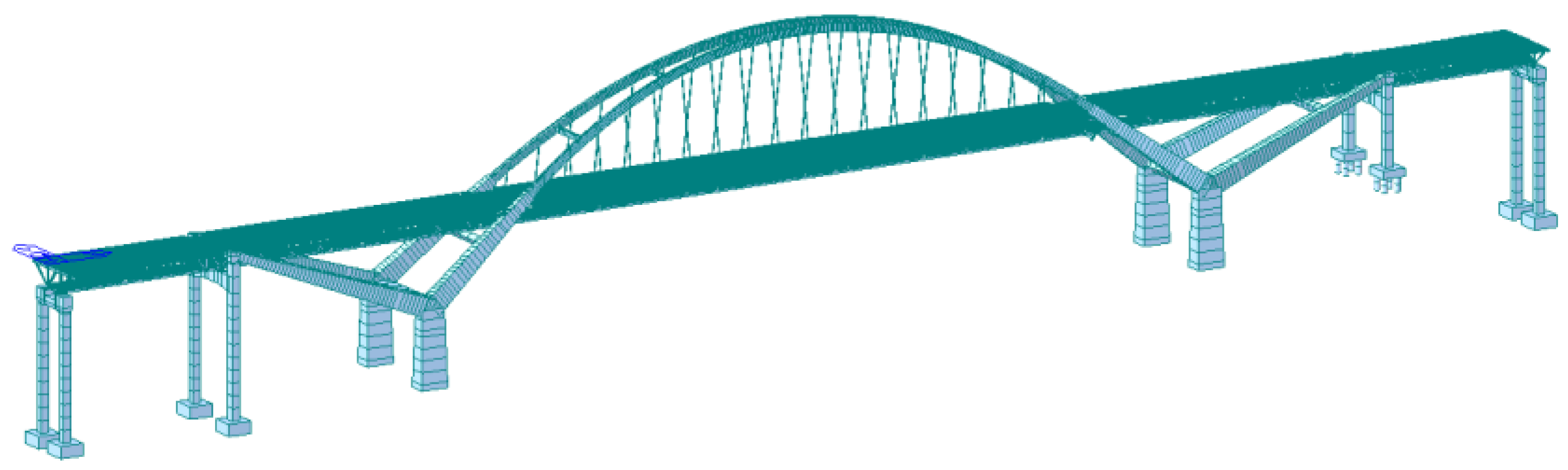
3.1. Bridge Subsystem
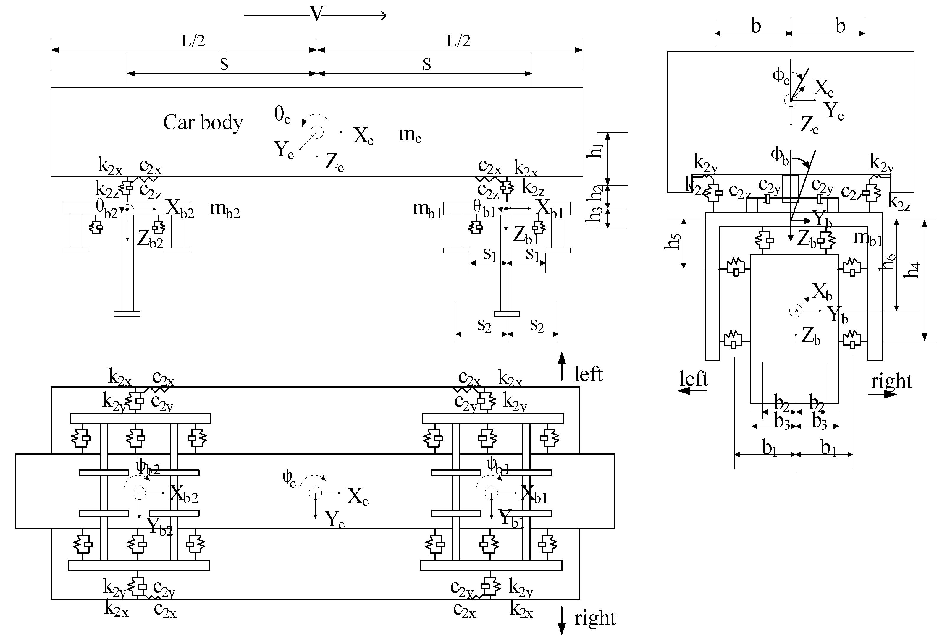
3.2. Monorail Train
- (1)
- The train body and two bogies are considered rigid bodies without any deformation.
- (2)
- The effects of variation in the vertical loads on the stiffness of the traveling wheel are neglected.
- (3)
- The wheels are in direct contact with the bridge deck.
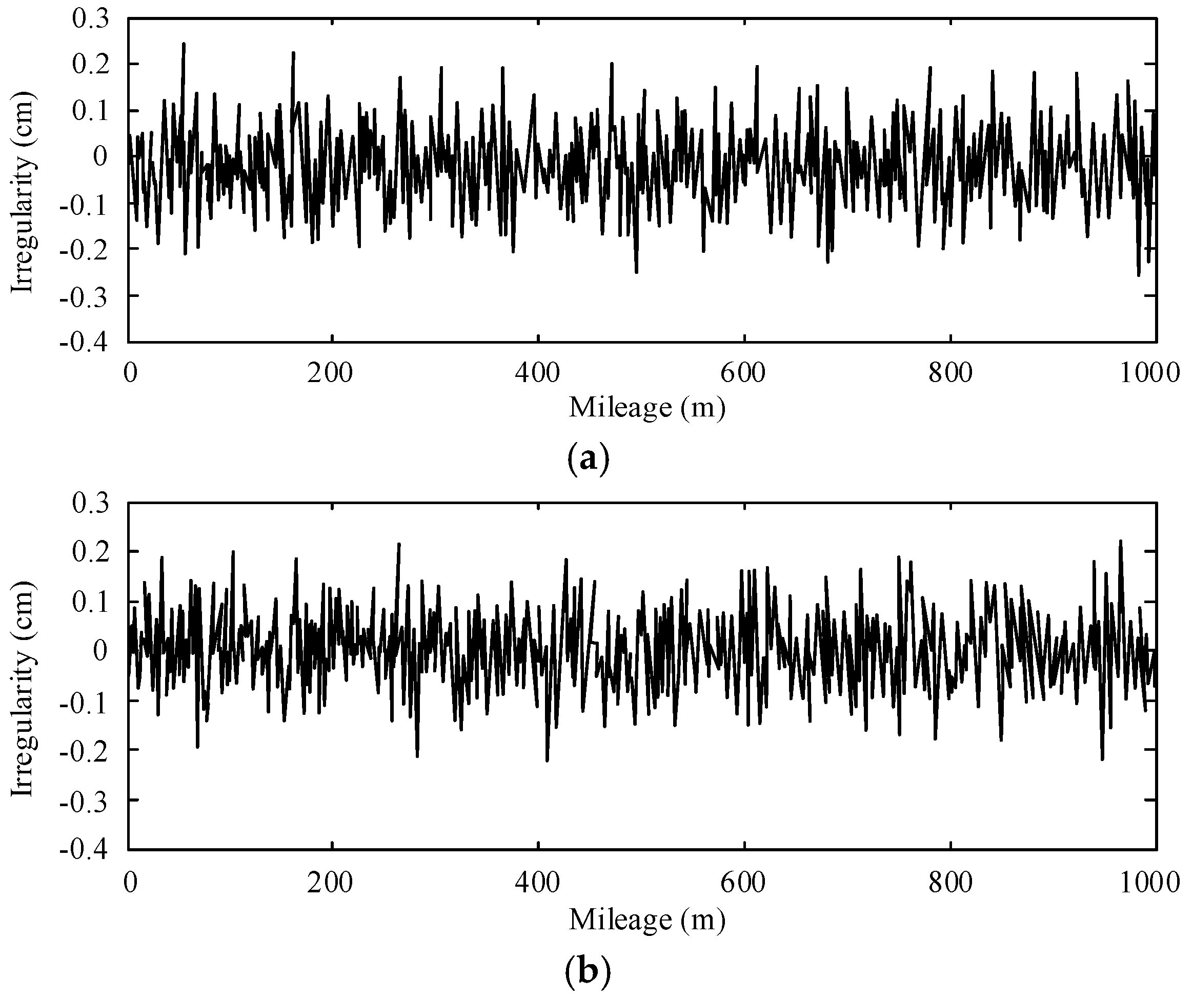
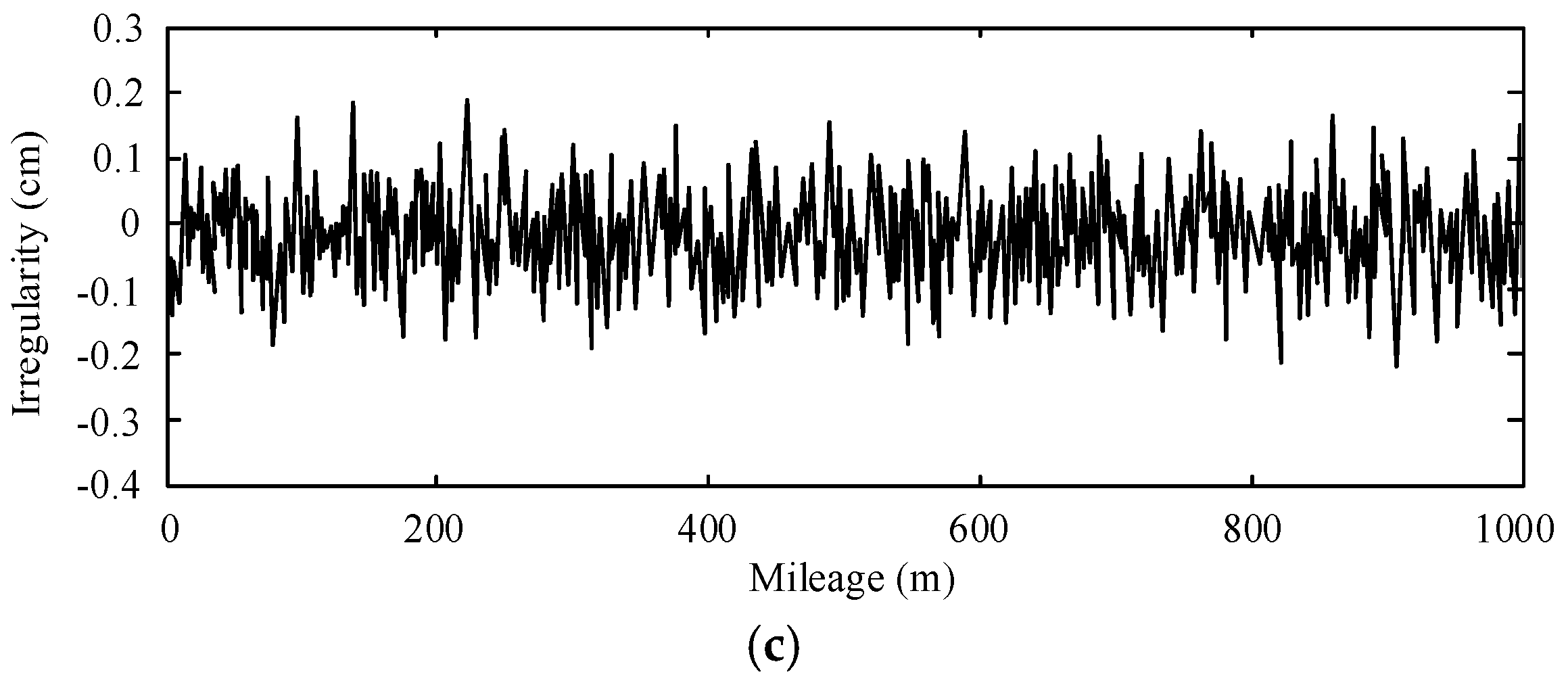
3.3. Track Irregularity
3.4. Monorail Train–Bridge Interaction
3.5. Investigated Cases
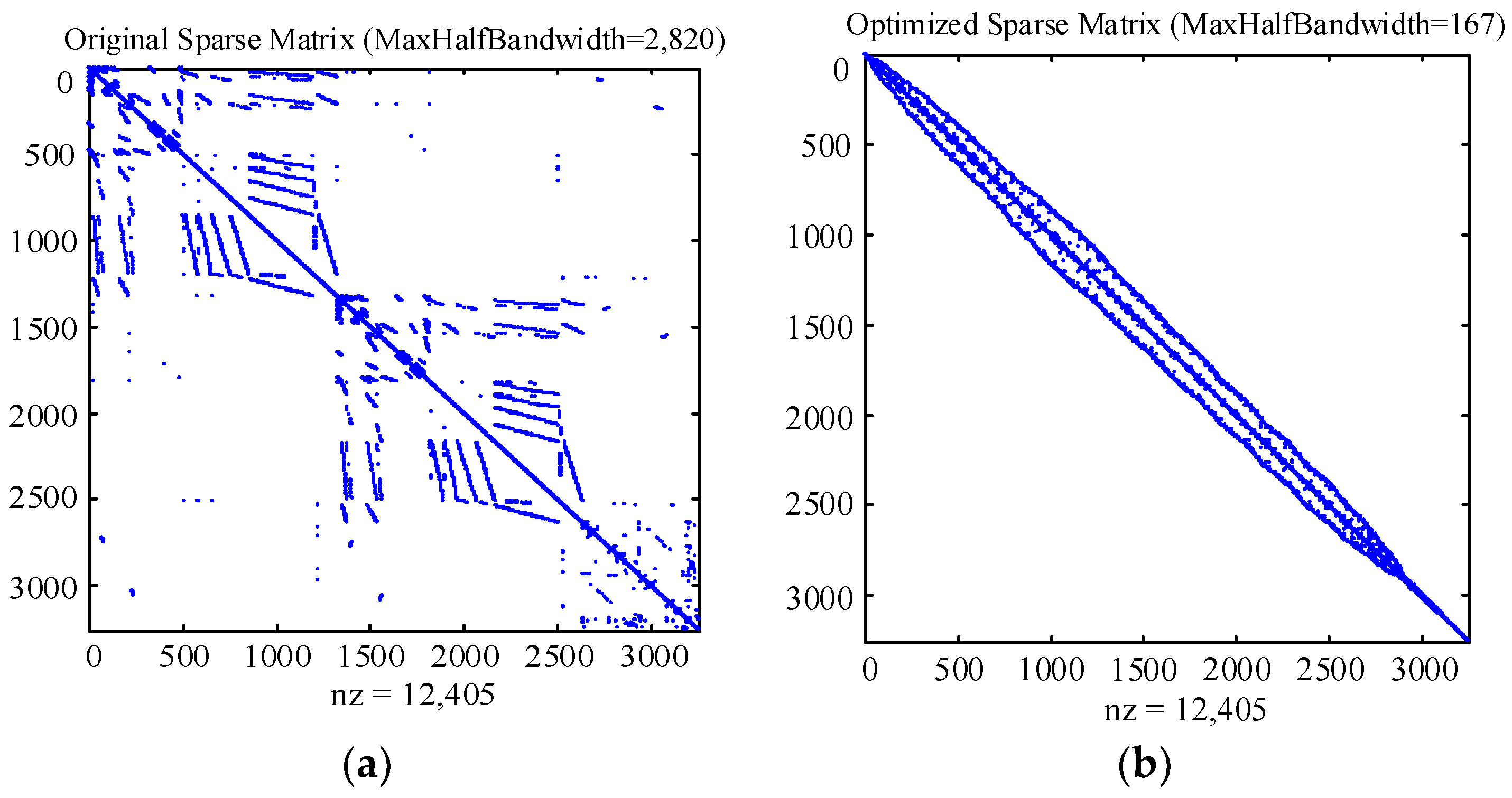
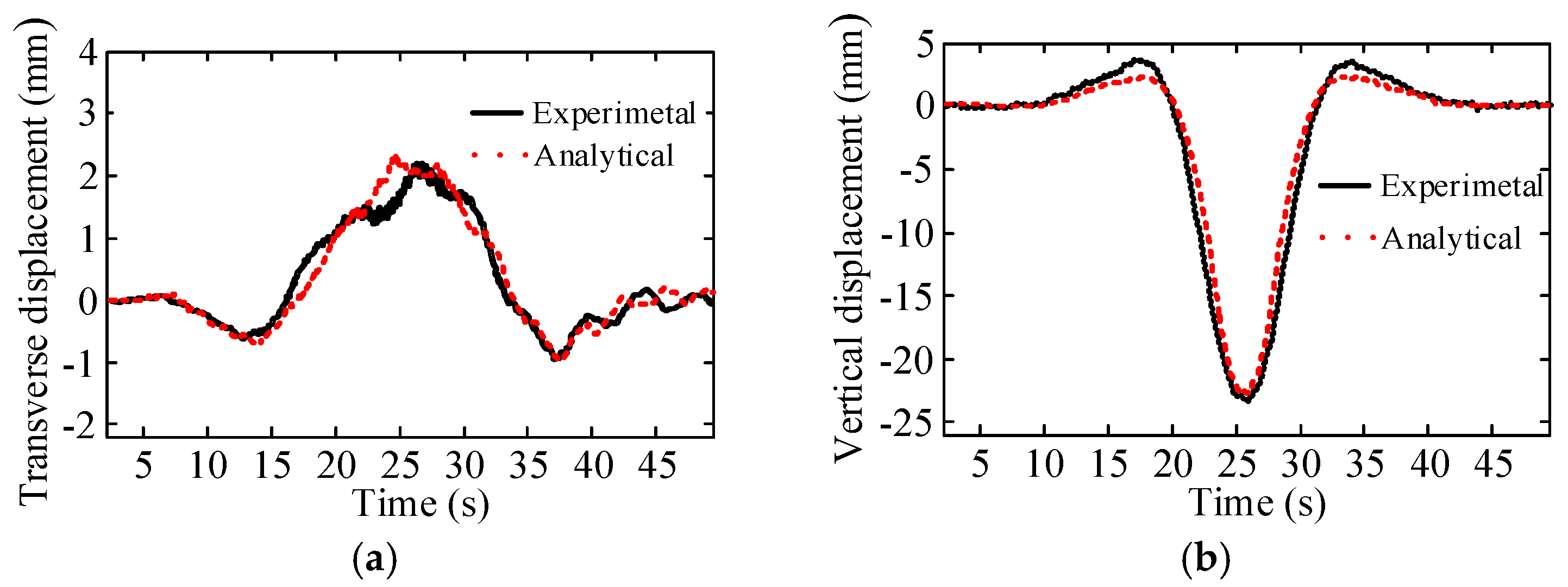
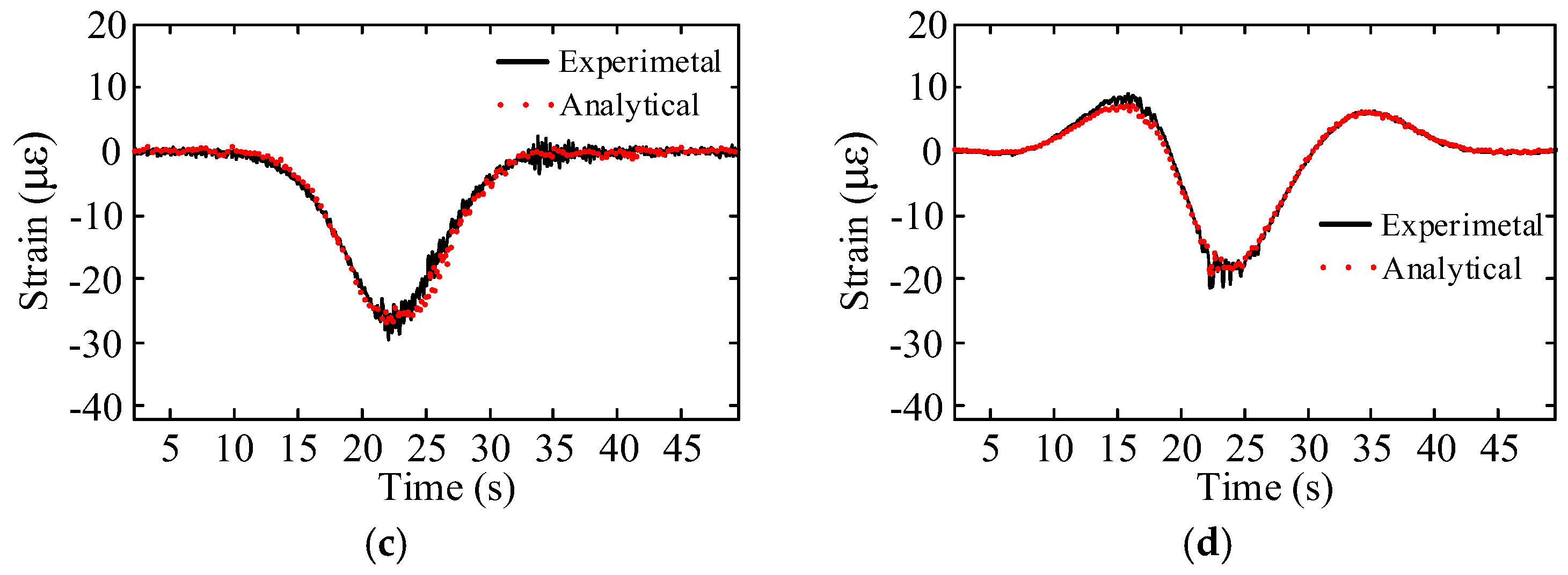
4. Model Optimization and Validation
5. Simulation Results and Discussions
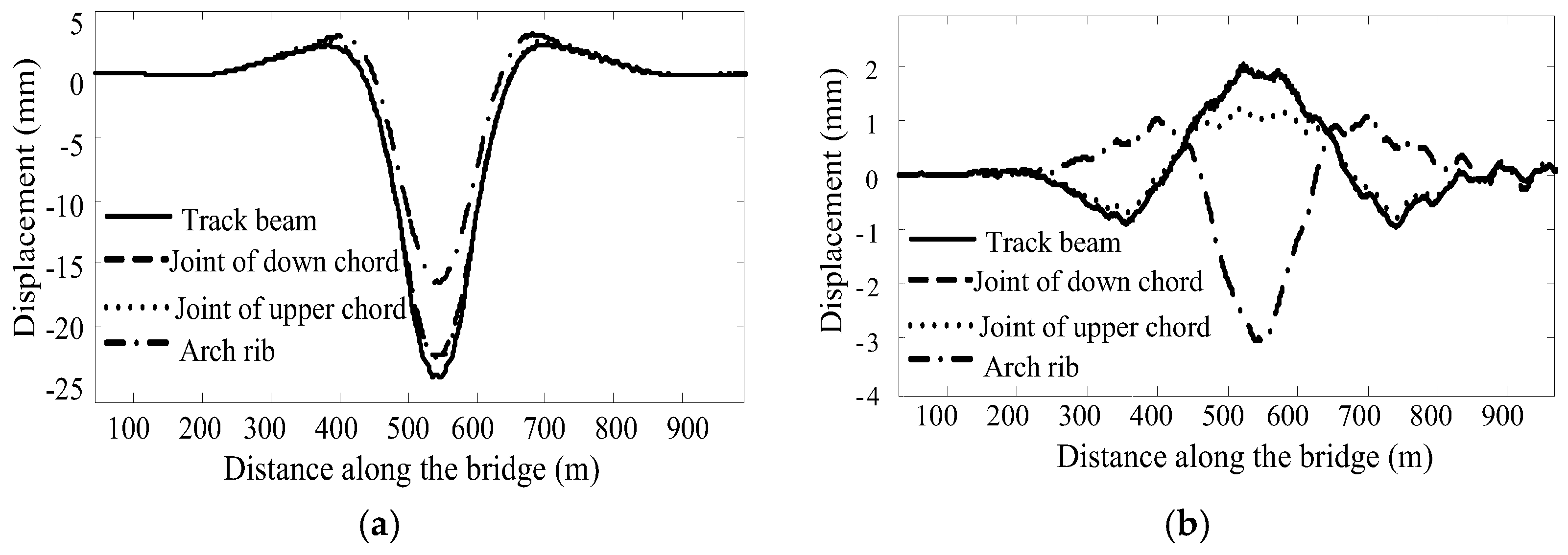
5.1. Displacements
5.2. Impact Factors
5.3. Accelerations
5.4. Effects of Train Braking
6. Evaluation of Riding Comfort
7. Conclusions
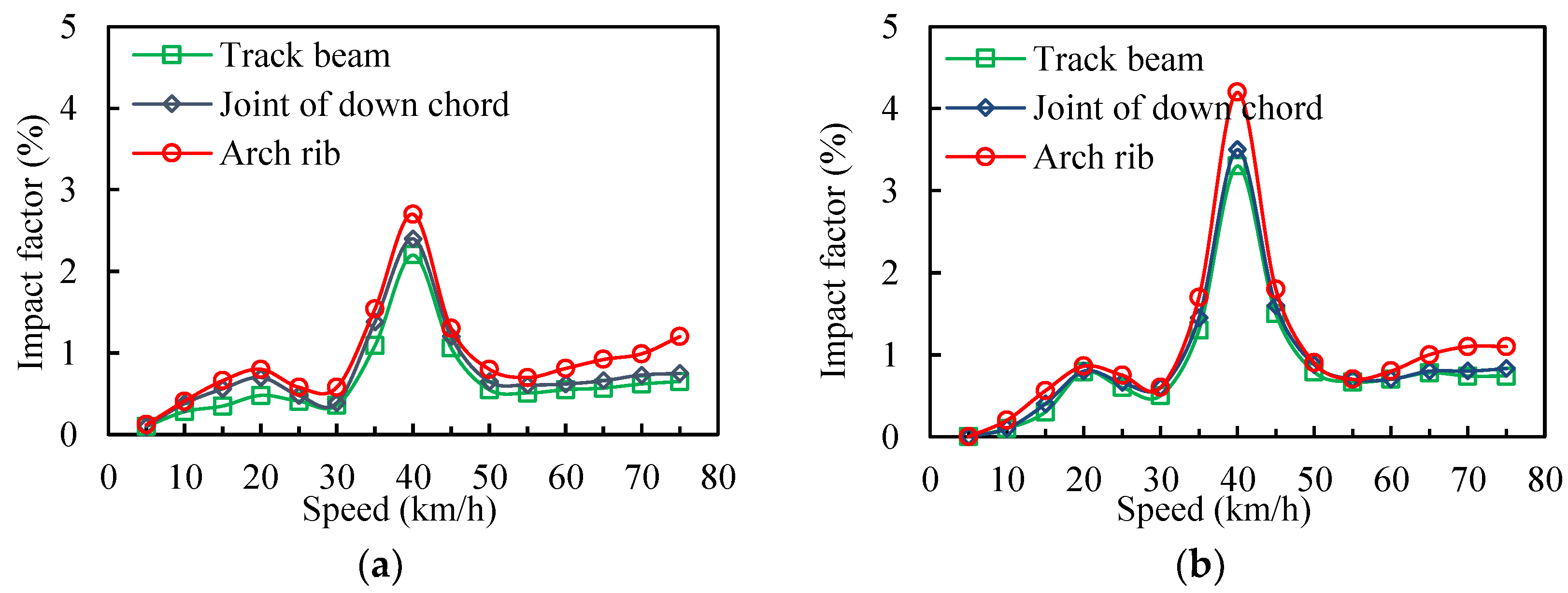
- The impact factor reaches the maximum values when the vehicle speed is 40 km/h in both the single line and double line loading cases. The largest impact factor is 4.2% in the double line case and 2.7% in the single line case, both achieved by the arch rib. Whether single line or double line loading is applied does not significantly affect the impact factor of the bridge.
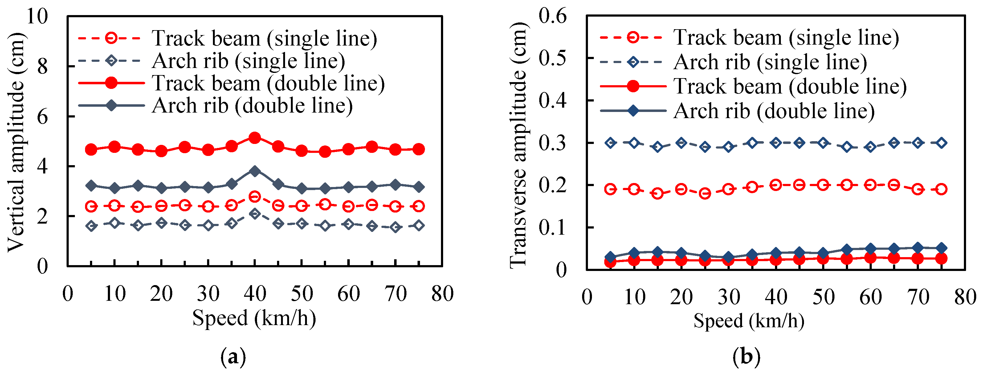
- Both the vertical and transverse amplitudes do not change significantly with the train’s speed when the speed is no more than 30 km/h. When the speed is increased to 40 km/h, the vertical amplitude is increased and a peak appeared, likely due to the resonance between the bridge and the train. The transverse amplitude is insensitive to the change of the train speed. When the loading case is changed from single line to double line, the vertical amplitude increases while the transverse amplitude of the bridge reduces. The transverse amplitude of the bridge approaches zero as two trains run on the double line, revealing that the transverse vibration of the bridge is mainly caused by eccentric train loadings.
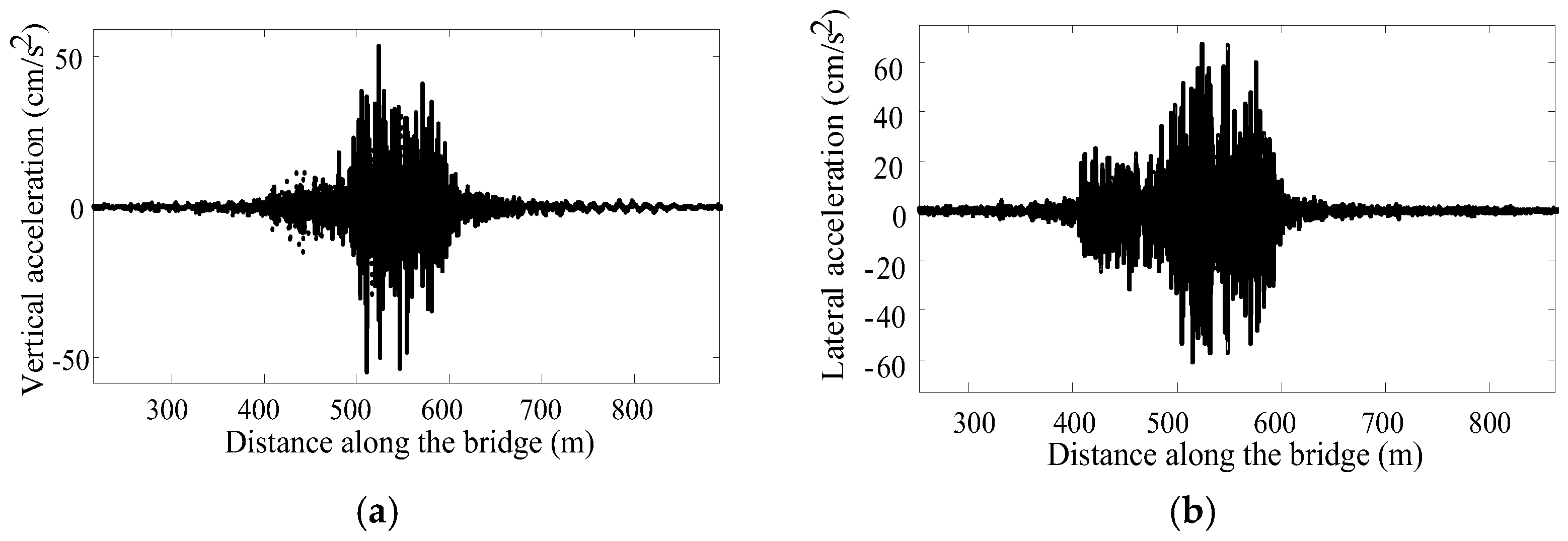
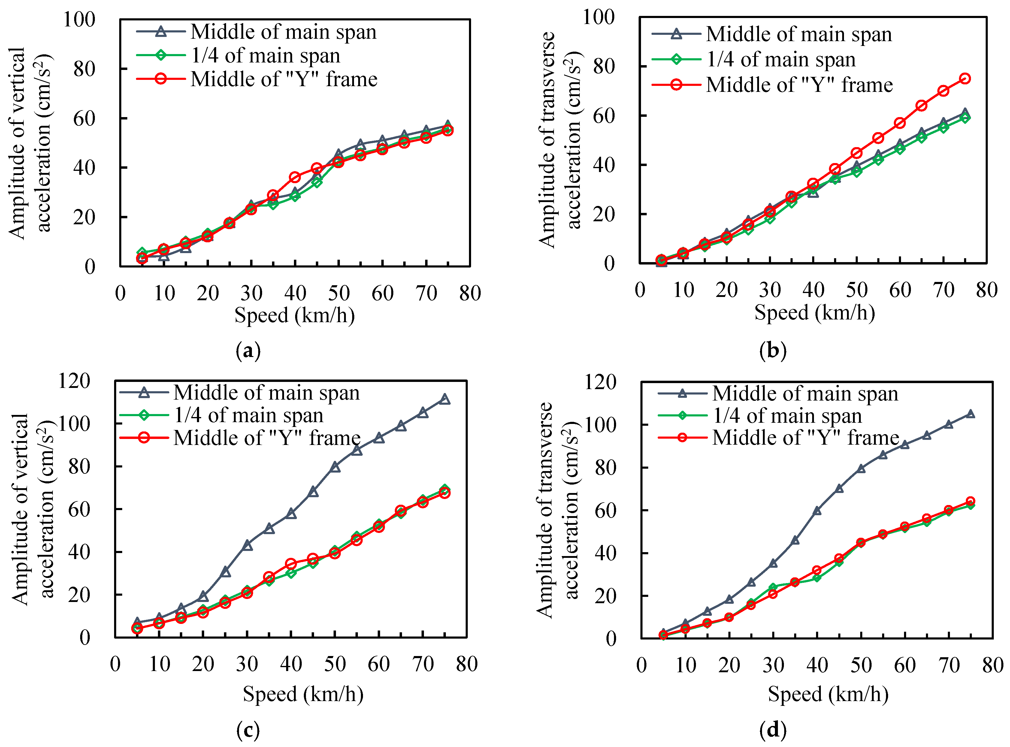
- The dynamic accelerations of the bridge approximately linearly increase with the train’s speed. In the single line loading case, the discrepancies of the amplitudes of the vertical and transverse accelerations of different parts of the bridge are no more than 18%. In the double line loading case, the amplitudes of the vertical and transverse accelerations of the quarter of main span and the middle of the Y-shape frame are still very close to each other, but the amplitudes of the vertical and transverse accelerations of the middle of the main span of the bridge are significantly greater than those of the quarter of the main span and the middle of the Y-shape frame. Their difference increases with the train’s speed and is up to 44% as the train’s speed is increased from 5 to 75 km/h. The acceleration of the track beam is much greater than that of the arch rib. The reason can be that the track beam is subjected to direct loading and the vehicle is coupled with the track beam, while the arch rib is subjected to indirect loading.
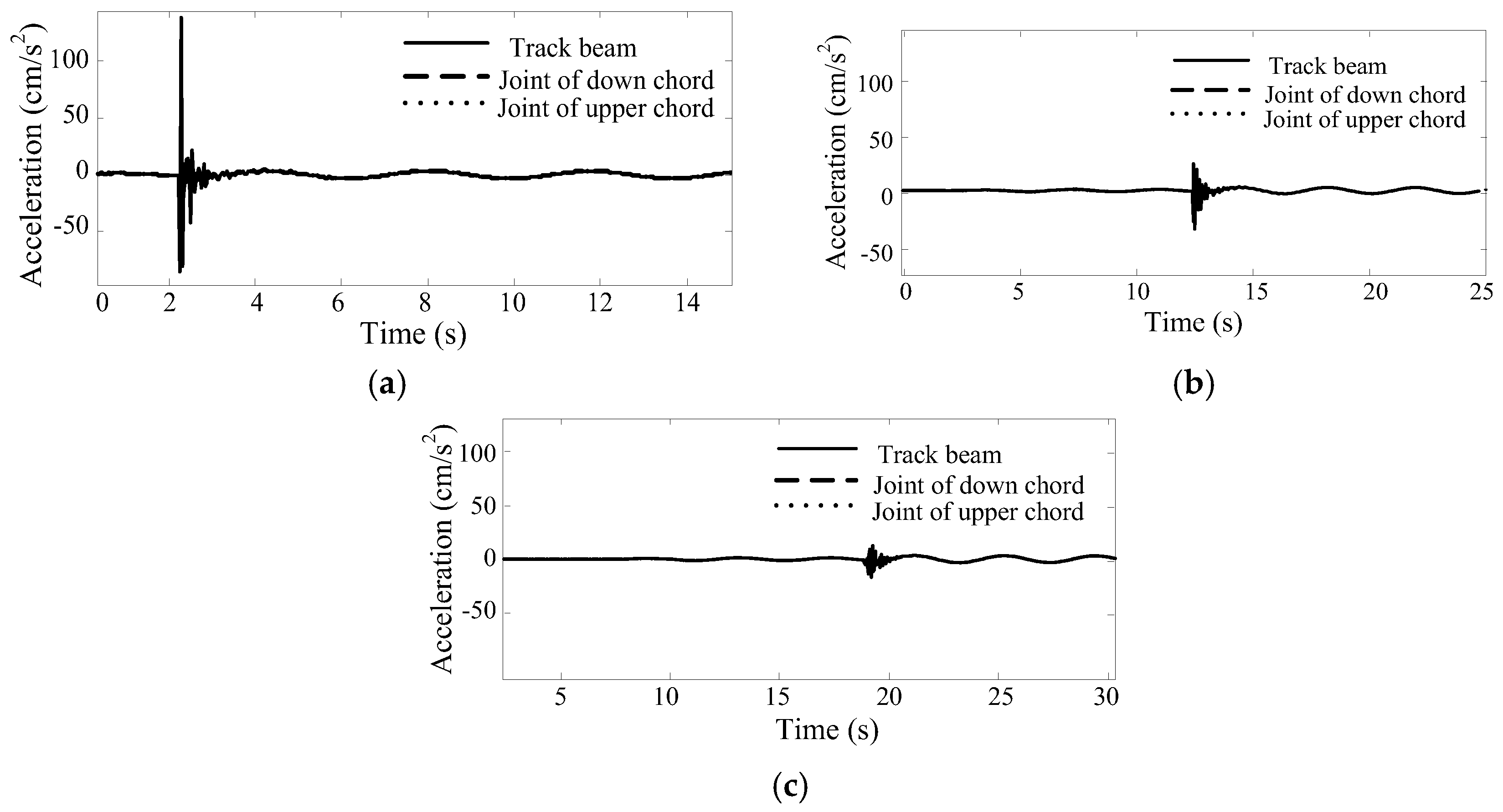
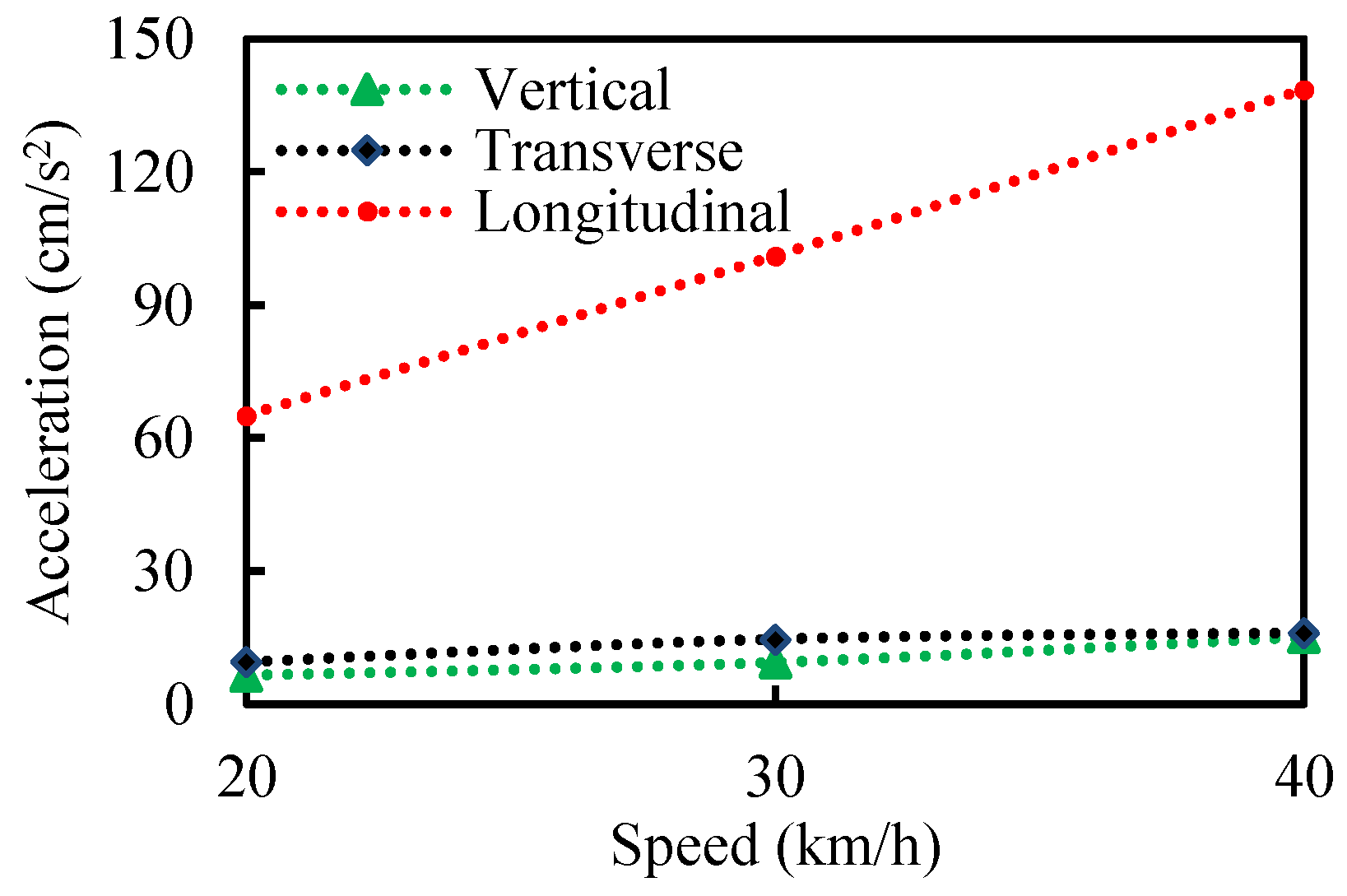
- The braking load mainly leads to larger longitudinal vibration of the bridge but its influence on the transverse and vertical vibration is less. When the braking load acts on the bridge, the longitudinal displacement and the vibration phase at each calculated position of the steel truss girder is consistent, that is, the steel truss girder makes longitudinal integral translational vibration. When the temporary impact occurs, the longitudinal accelerations of each calculated position varies greatly. As the distance from the braking position increases, the longitudinal acceleration of the steel truss girder becomes smaller.
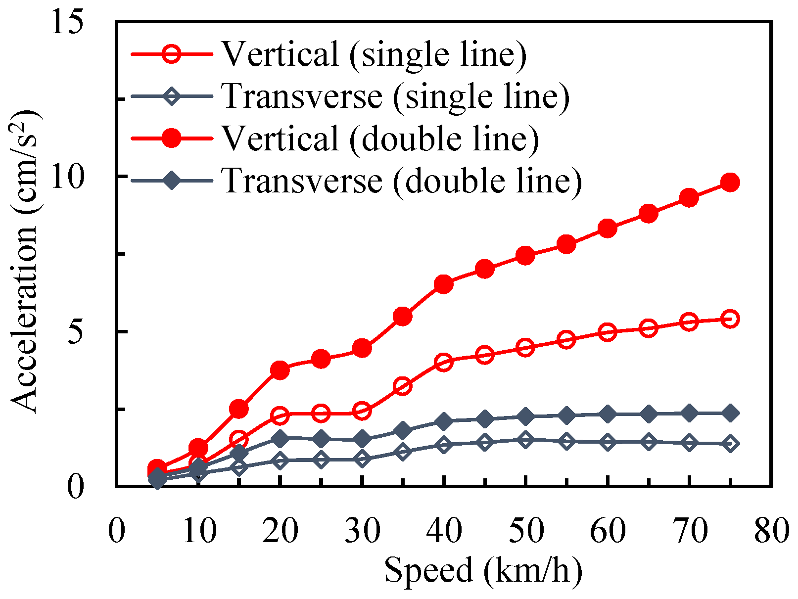
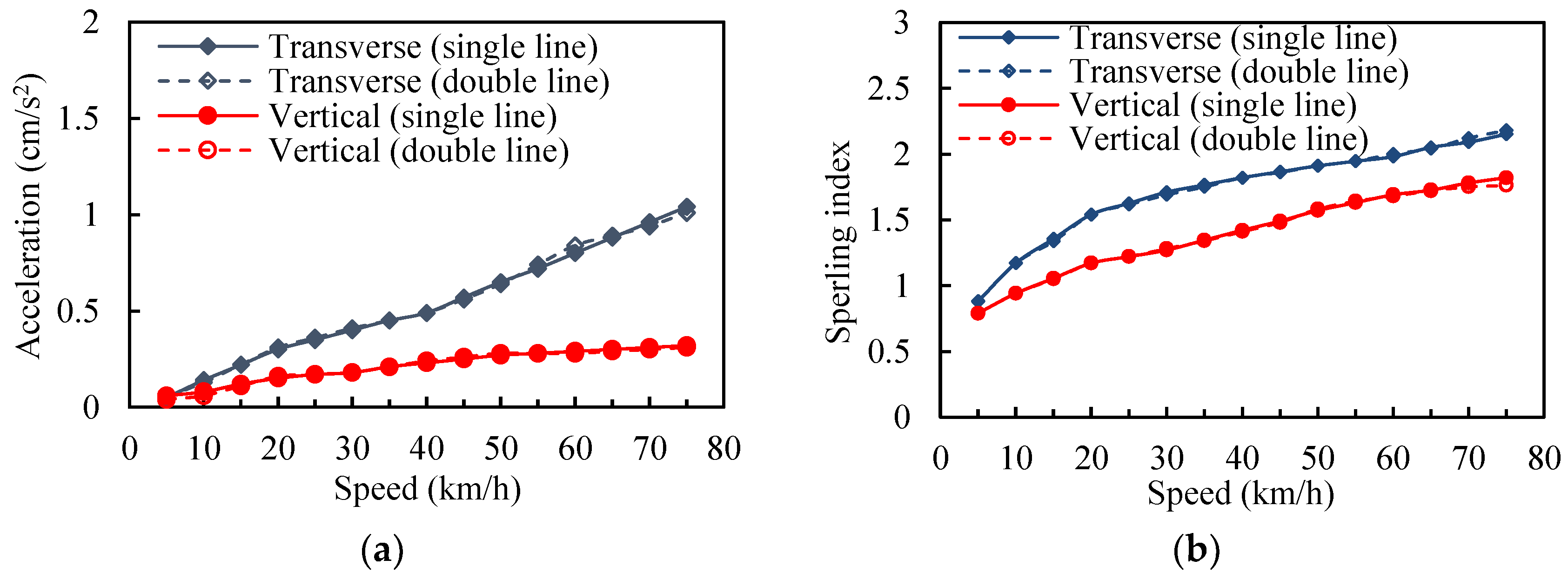
- The acceleration of the vehicles increases with the vehicle speed, not the number of vehicles. The transverse acceleration of the vehicle is significantly greater than the vertical one, and the transverse comfort is worse than the vertical comfort. The maximum transverse acceleration of the vehicle is 1.01cm/s2. The grade of the vehicle running stability is excellent.
Acknowledgments
Author Contributions
Conflicts of Interest
References
- Lee, C.H.; Kim, C.W.; Kawatani, M. Dynamic response analysis of monorail bridges under moving trains and riding comfort of trains. Eng. Struct. 2005, 27, 1999–2013. [Google Scholar] [CrossRef]
- Yang, S.C.; Hwang, S.H. Train-track-bridge interaction by coupling direct stiffness method and mode superposition method. J. Bridge Eng. 2016, 21, 04016058. [Google Scholar] [CrossRef]
- Wang, S.J.; Xu, Z.D.; Li, S.; Dyke, S.J. Safety and stability of light-rail train running on multispan bridges with deformation. J. Bridge Eng. 2016, 21, 06016004. [Google Scholar] [CrossRef]
- Dinh, V.N.; Kim, K.D.; Warnitchai, P. Dynamic analysis of three-dimensional bridge-high-speed train interactions using a wheel-rail contact model. Eng. Struct. 2009, 31, 3090–3106. [Google Scholar] [CrossRef]
- Zhang, N.; Xia, H.; Guo, W.W. Vehicle-bridge interaction analysis under high-speed trains. J. Sound Vib. 2008, 309, 407–425. [Google Scholar] [CrossRef]
- Wang, H.; Silvast, M.; Markinei, V.; Wiljanen, B. Analysis of the Dynamic Wheel Loads in Railway Transition Zones Considering the Moisture Condition of the Ballast and Subballast. Appl. Sci. 2017, 7, 1208. [Google Scholar] [CrossRef]
- Shi, X.M.; Cai, C.S. Simulation of dynamic effects of vehicles on pavement using a 3D interaction model. J. Transp. Eng. 2009, 135, 736–744. [Google Scholar] [CrossRef]
- Darestani, M.Y.; Thambiratnam, D.P.; Nataatmadja, A.; Baweja, D. Structural response of concrete pavements under moving truck loads. J. Transp. Eng. 2007, 133, 670–676. [Google Scholar] [CrossRef]
- Xia, C.Y.; Lei, J.Q.; Zhang, N.; Xia, H.; Roeck, G.D. Dynamic analysis of a coupled high-speed train and bridge system subjected to collision load. J. Sound Vib. 2012, 331, 2334–2347. [Google Scholar] [CrossRef]
- Olmos, J.M.; Astiz, M.A. Analysis of the lateral dynamic response of high pier viaducts under high-speed train travel. Eng. Struct. 2013, 56, 1384–1401. [Google Scholar] [CrossRef]
- Xu, Y.L.; Xia, H.; Yan, Q.S. Dynamic response of suspension bridge to high wind and running train. J. Bridge Eng. 2003, 8, 46–55. [Google Scholar] [CrossRef]
- Malm, R.; Andersson, A. Field testing and simulation of dynamic properties of a tied arch railway bridge. Eng. Struct. 2006, 28, 143–152. [Google Scholar] [CrossRef]
- Kwon, S.D.; Lee, J.S.; Moon, J.W.; Kim, M.Y. Dynamic interaction analysis of urban transit maglev vehicle and guideway suspension bridge subjected to gusty wind. Eng. Struct. 2008, 30, 3445–3456. [Google Scholar] [CrossRef]
- Zhong, H.; Yang, M.; Gao, Z. Dynamic responses of prestressed bridge and vehicle through bridge-vehicle interaction analysis. Eng. Struct. 2015, 87, 116–125. [Google Scholar] [CrossRef]
- Kaliyaperumal, G.; Imam, B.; Righiniotis, T. Advanced dynamic finite element analysis of a skew steel railway bridge. Eng. Struct. 2011, 33, 181–190. [Google Scholar] [CrossRef]
- Madrazo-Aguirre, F.; Ruiz-Teran, A.M.; Wadee, A. Dynamic behavior of steel-concrete composite under-deck cable-stayed bridges under the action of moving loads. Eng. Struct. 2015, 103, 260–274. [Google Scholar] [CrossRef]
- Fu, C. Dynamic behavior of a simply supported bridge with a switching crack subjected to seismic excitations and moving trains. Eng. Struct. 2016, 110, 59–69. [Google Scholar] [CrossRef]
- Gou, H.Y.; Shi, X.Y.; Zhou, W.; Cui, K.; Pu, Q.H. Dynamic performance of continuous railway bridges: Numerical analyses and field tests. Proc. Inst. Mech. Eng. F J. Rail Rapid Transit. 2018, 232, 936–955. [Google Scholar] [CrossRef]
- Gou, H.Y.; Long, H.; Bao, Y.; Chen, G.D.; Pu, Q.H.; Kang, R. Experimental and numerical studies on stress distributions in girder-arch-pier connections of long-span continuous rigid frame arch railway bridge. J. Bridge Eng. 2018, in press. [Google Scholar]
- Gou, H.Y.; He, Y.N.; Zhou, W.; Bao, Y.; Chen, G.D. Experimental and numerical investigations of the dynamic responses of an asymmetrical arch railway bridge. Proc. Inst. Mech. Eng. F J. Rail Rapid Transit. 2018, in press. [Google Scholar] [CrossRef]
- Gou, H.Y.; Long, H.; Bao, Y.; Chen, G.D.; Pu, Q.H. Dynamic behavior of hybrid framed arch railway bridge under moving trains. Steel Compos. Struct. 2018, in press. [Google Scholar]
- Gou, H.Y.; Wang, W.; Shi, X.Y.; Pu, Q.H.; Kang, R. Behavior of steel-concrete composite cable anchorage system. Steel Compos. Struct. 2018, 26, 115–123. [Google Scholar]
- Cui, K.; Qin, X. Virtual reality research of the dynamic characteristics of soft soil under metro vibration loads based on BP neural networks. Neural Comput. Appl. 2017, 1–10. [Google Scholar] [CrossRef]
- Cui, C.; Zhang, Q.H.; Luo, Y.; Hao, H.; Li, J. Fatigue Reliability Evaluation of Deck-to-Rib Welded Joints in OSD Considering Stochastic Traffic Load and Welding Residual Stress. Int. J. Fatigue 2018, 111, 151–160. [Google Scholar] [CrossRef]
- Zhang, Q.H.; Liu, Y.M.; Bao, Y.; Jia, D.L.; Bu, Y.Z.; Li, Q. Fatigue performance of orthotropic steel-concrete composite deck with large-size longitudinal trough. Eng. Struct. 2017, 150, 864–874. [Google Scholar] [CrossRef]
- Wang, H.; Zhu, E.; Chen, Z. Dynamic Response Analysis of the Straddle-Type Monorail Bridge-Vehicle Coupling System. Urban Rail Transit 2017, 3, 172–181. [Google Scholar] [CrossRef]
- Goda, K.; Nishigaito, T.; Hiraishi, M.; Iwasaki, K. A curving simulation for a monorail car. In Proceedings of the 2000 ASME/IEEE Joint Railroad Conference, Newark, NJ, USA, 4–6 April 2000; pp. 171–177. [Google Scholar]
- Lee, C.H.; Kawatani, M.; Kim, C.W.; Nishimura, N.; Kobayashi, Y. Dynamic response of a monorail steel bridge under a moving train. J. Sound Vib. 2006, 294, 562–579. [Google Scholar] [CrossRef]
- Chinese National Bureau of Standards. Railway Vehicles-Specification for Evaluation the Dynamic Performance and Accreditation Test; Chinese Railway Ministry: Beijing, China, 1985. (In Chinese) [Google Scholar]
- Zeng, Q.Y.; Yang, P. The “set-in-right position” rule for forming structural matrices and truss segment finite element method for spatial analysis of truss girder. J. China Railw. Soc. 1986, 8, 48–58. [Google Scholar]
- Li, X.Z.; Lei, H.J.; Zhu, Y. Analysis of rayleigh damping parameters in a dynamic system of vehicle-track-bridge. J. Vib. Shock 2013, 32. [Google Scholar] [CrossRef]
- Mitsuo, K.; Chul-woo, K. Computer simulation for dynamic wheel loads of heavy vehicles. Struct. Eng. Mech. 2001, 12, 409–428. [Google Scholar]
- Liu, Z.; Luo, S.; Ma, W.; Song, R. Application research of track irregularity PSD in the high-speed train dynamic simulation. In Proceedings of the International Conference on Transportation Engineering, Chengdu, China, 25–27 July 2009; pp. 2845–2850. [Google Scholar]
- Liu, X.; Lian, S.; Yang, W. Influence analysis of irregularities on vehicle dynamic response on curved track of speed-up railway. In Proceedings of the Third International Conference on Transportation Engineering, Chengdu, China, 23–25 July 2011; pp. 2643–2648. [Google Scholar]
- Guo, W.H.; Xu, Y.L. Fully computerized approach to study cable-stayed bridge-vehicle interaction. J. Sound Vib. 2001, 248, 745–761. [Google Scholar] [CrossRef]
- Arkars, G.; Dhatt, G. An automatic node relabeling scheme for minimizing a matrix or network bandwidth. Int. J. Numer. Meth. Eng. 1976, 10, 787–797. [Google Scholar]
- He, R.; He, W.; Geng, G.H. Research on Dynamic Properties of Concrete Steel Tubular Arch Bridge Based on ANSYS. Appl. Mech. Mater. 2011, 71–78, 3233–3236. [Google Scholar] [CrossRef]
- Lee, I.W.; Kim, C.H.; Kim, B.W.; Cho, S.W. Determination of natural frequencies and mode shapes of structures using subspace iteration method with accelerated Starting vectors. J. Struct. Eng. 2005, 131, 1146–1149. [Google Scholar]
- Gou, H.Y.; Zhou, W.; Chen, G.D.; Bao, Y.; Pu, Q.H. In-situ test and dynamic analysis of a double-deck tied-arch bridge. Steel Compos. Struct. 2018, 27, in press. [Google Scholar]
- Mottershead, J.E.; Link, M.; Friswell, M.I. The sensitivity method in finite element model updating: A tutorial. Mech. Syst. Signal Process. 2011, 25, 2275–2296. [Google Scholar] [CrossRef]
- Carpinteri, A.; Lacidogna, G.; Accornero, F. Evolution of fracturing process in masonry arches. J. Struct. Eng. 2015, 141, 1–10. [Google Scholar] [CrossRef]
- Block, P.; Dejong, M.J.; Ochsendorf, J. As hangs the flexible line: Equilibrium of masonry arches. Nexus Netw. J. 2006, 8, 9–19. [Google Scholar] [CrossRef]
- Chinese Railway Ministry. Code for Rating Existing Railway Bridges; Chinese Railway Ministry: Beijing, China, 2004. [Google Scholar]
- Graa, M.; Nejlaoui, M.; Houidi, A.; Affi, Z.; Romdhane, L. Modeling and control for lateral rail vehicle dynamic vibration with comfort evaluation. Adv. Acoust. Vib. 2017, 5, 89–100. [Google Scholar]


| Component | Young’s Modulus (MPa) | Poisson’s Ratio | Unit Weight (kN/m3) |
|---|---|---|---|
| Main arch | 2.06 × 10⁵ | 0.3 | 78.5 |
| Steel truss girder | 2.06 × 10⁵ | 0.3 | 78.5 |
| Y-shaped rigid frame | 3.60 × 10⁴ | 0.2 | 26.0 |
| Main pier | 3.45 × 10⁴ | 0.2 | 26.0 |
| Abutment pier | 3.25 × 10⁴ | 0.2 | 25.0 |
| Suspenders and tied bars | 1.95 × 10⁵ | 0.3 | 78.5 |
| Foundation | 3.00 × 10⁴ | 0.2 | 25.0 |
| Rigid | Yawing | Vertical Settlement | Side-Rolling | Head Shaking | Nodding |
|---|---|---|---|---|---|
| Car body | yc | zc | φc | ψc | θc |
| Bogie | yb | zb | φb | ψb | θb |
| Parameters | Value | Unit |
|---|---|---|
| Mass of the bogie (mb) | 6170 | kg |
| Moment of inertia of the bogie on the X-axis (Ibφ) | 2850 | kg m2 |
| Moment of inertia of the bogie on the Y-axis (Ibθ) | 4650 | kg m2 |
| Moment of inertia of the bogie on the Z-axis (Ibψ) | 6550 | kg m2 |
| Mass of the car body (mc) | 28,800 | kg |
| Moment of inertia of the car body on the X-axis (Icφ) | 53,900 | kg m2 |
| Moment of inertia of the car body on the Y-axis (Icθ) | 539,000 | kg m2 |
| Moment of inertia of the car body on the Z-axis (Icψ) | 530,000 | kg m2 |
| Stiffness of the traveling wheel (kr) | 1180 | kN/m |
| Stiffness of the steering wheel (kg) | 980 | kN/m |
| Stiffness of the stabilizing wheel (ks) | 980 | kN/m |
| Damping of the traveling wheel (cr) | 26.1 | kN s/m |
| Damping of the steering wheel (cg) | 186 | kN s/m |
| Damping of the stabilizing wheel (cs) | 186 | kN s/m |
| Longitudinal stiffness of the secondary spring (k2x) | 130 | kN/m |
| Transverse stiffness of the secondary spring (k2y) | 130 | kN/m |
| Vertical stiffness of the secondary spring (k2z) | 160 | kN/m |
| Longitudinal damping of the secondary suspension system (c2x) | 333.6 | kN s/m |
| Transverse damping of the secondary suspension system (c2y) | 333.6 | kN s/m |
| Vertical damping of the secondary suspension system (c2z) | 22.8 | kN s/m |
| Vertical distance between the center of the car body and the center of the secondary spring (h1) | 0.529 | m |
| Vertical distance between the center of the bogie and the center of the secondary spring (h2) | 0.352 | m |
| Transverse distance between the center of the car body and the upper endpoint of the secondary spring (b) | 1.025 | m |
| Longitudinal distance between the center of the car body and the upper endpoint of the secondary spring (s) | 4.8 | m |
| Height between the centers of the bogie and the traveling wheel (h3) | −0.221 | m |
| Transverse distance between the centers of the bogie and the traveling wheel (b2) | 0.2 | m |
| Longitudinal distance between the centers of the bogie and the traveling wheel (s1) | 0.75 | m |
| Height between the centers of the bogie and the steering wheel (h5) | −0.061 | m |
| Transverse distance between the centers of the bogie and the steering wheel (b1) | 0.782 | m |
| Longitudinal distance between the centers of the bogie and the steering wheel (s2) | 1.2 | m |
| Height between the centers of the bogie and the stabilizing wheel (h4) | 1.025 | m |
| Transverse distance between the centers of the bogie and the stabilizing wheel (b1) | 0.782 | m |
| Half-width of the track beam (b3) | 0.345 | m |
| Height between the centers of the bogie and the track beam (h6) | 0.725 | m |
| Length of the vehicle (L) | 15.5 | m |
| Mode No. | Frequency (Hz) | Discrepancy | Vibration Mode | Mode Shape | |
|---|---|---|---|---|---|
| ANSYS | SCP | ||||
| 1 | 0.317 | 0.318 | 0.3% | Transverse deformation |  |
| 2 | 0.388 | 0.389 | 0.3% | Longitudinal deformation |  |
| 3 | 0.419 | 0.420 | 0.1% | Transverse deformation |  |
| 4 | 0.515 | 0.516 | 0.1% | Longitudinal deformation |  |
| 5 | 0.537 | 0.537 | 0.0% | Longitudinal deformation |  |
| 6 | 0.609 | 0.610 | 0.2% | Vertical deformation |  |
| Wz | Riding Comfort | Wz | Riding Quality |
|---|---|---|---|
| 1 | Just feel | 1 | Excellent |
| 2 | Obvious feeling | 2 | Good |
| 2.5 | More obviously without uncomfortable feeling | 3 | Meet the requirement |
| 3 | Strong and abnormal but can tolerate | 4 | Allow operation |
| 3.25 | Extremely abnormal | 4.5 | Not allowed to run |
| 3.5 | Extremely abnormal and cannot endure for long | 5 | Dangerous |
| 4 | Very uncomfortable and it’s harmful to stand for long | - | - |
| 1 | Just feel | 1 | Excellent |
| Running Stability Grade | Evaluation Level | Sperling Index | |
|---|---|---|---|
| Passenger Train | Freight Train | ||
| Class 1 | Excellent | <2.5 | <3.5 |
| Class 2 | Good | 2.5–2.75 | 3.5–4.0 |
| Class 3 | Qualified | 2.75–3 | 4.0–4.25 |
© 2018 by the authors. Licensee MDPI, Basel, Switzerland. This article is an open access article distributed under the terms and conditions of the Creative Commons Attribution (CC BY) license (http://creativecommons.org/licenses/by/4.0/).
Share and Cite
Gou, H.; Zhou, W.; Yang, C.; Bao, Y.; Pu, Q. Dynamic Response of a Long-Span Concrete-Filled Steel Tube Tied Arch Bridge and the Riding Comfort of Monorail Trains. Appl. Sci. 2018, 8, 650. https://doi.org/10.3390/app8040650
Gou H, Zhou W, Yang C, Bao Y, Pu Q. Dynamic Response of a Long-Span Concrete-Filled Steel Tube Tied Arch Bridge and the Riding Comfort of Monorail Trains. Applied Sciences. 2018; 8(4):650. https://doi.org/10.3390/app8040650
Chicago/Turabian StyleGou, Hongye, Wen Zhou, Changwei Yang, Yi Bao, and Qianhui Pu. 2018. "Dynamic Response of a Long-Span Concrete-Filled Steel Tube Tied Arch Bridge and the Riding Comfort of Monorail Trains" Applied Sciences 8, no. 4: 650. https://doi.org/10.3390/app8040650
APA StyleGou, H., Zhou, W., Yang, C., Bao, Y., & Pu, Q. (2018). Dynamic Response of a Long-Span Concrete-Filled Steel Tube Tied Arch Bridge and the Riding Comfort of Monorail Trains. Applied Sciences, 8(4), 650. https://doi.org/10.3390/app8040650