Lyapunov Equivalent Representation Form of Forced, Damped, Nonlinear, Two Degree-of-Freedom Systems

Featured Application

The qualitative and quantitative dynamic behavior of two degree-of-freedom nonlinear systems can be studied by using their corresponding decoupled one degree of freedom Duffing type equivalent representation forms in the sense of Lyapunov, with the advantage of capturing amplitude-dependent nonlinear mode shapes.

Abstract

The aim of this paper focuses on finding equivalent representation forms of forced, damped, two degree-of-freedom, nonlinear systems in the sense of Lyapunov by using a nonlinear transformation approach that provides decoupled, forced, damped, nonlinear equations of the Duffing type, under the assumption that the driving frequency and the external forces are equal in both systems. The values of Lyapunov characteristic exponents (LCEs), Lyapunov largest exponents (LLE), and time-amplitude and frequency-amplitude curves computed from numerical integration solutions, indicate that the decoupled Duffing-type equations are equivalent, in the sense of Lyapunov, to the original dynamic system, since both set of motion equations tend to have the same qualitative and quantitative behaviors.

1. Introduction

Minorsky [1], Caughey [2], Iwan [3,4], Sinha and Srinivasan [5], Agrwal and Denman [6], Yuste and Sánchez [7,8], Cai [9], Farzaneh and Tootoonchi [10], and many others have reported approaches that replace linear and nonlinear dynamic systems by equivalent ones with known solutions that are closed to the original system, which produce the same oscillations that appear in the original equations of motion. . There, the authors focused on using linearization, weighted mean-square, and least squares techniques to determine the equivalent expressions that provide solutions with the same quantitative and qualitative original system dynamics response behavior.

On the other hand, a nonlinear transformation approach that is based on a cubication method, was recently introduced to obtain the equivalent representation form of conservative two degree-of-freedom nonlinear oscillators [11]. There, the authors developed an approach to replace a two degree-of-freedom homogeneous, undamped system by another equivalent system with known solutions that were closed to the original one. In that approach, they first replaced the system restoring forces by polynomial expressions and then used a transformation technique to replace the resulting equations by two uncoupled nonlinear differential equations of the Duffing type. Here, some steps of that approach are used to convert forced, damped, nonlinear systems of the form [12,13,14,15]

$$\left[\begin{array}{cc}{m}_1& 0\\ 0& m_2\end{array}\right]\left\{\begin{array}{c}{\ddot{x}}_1\\ {\ddot{x}}_2\end{array}\right\}+\left[\begin{array}{cc}{c}_{11}& c_{12}\\ c_{21}& c_{22}\end{array}\right]\left\{\begin{array}{c}{\dot{x}}_1\\ {\dot{x}}_2\end{array}\right\}+\left[\begin{array}{cc}{k}_{11}& k_{12}\\ k_{21}& k_{22}\end{array}\right]\left\{\begin{array}{c}{x}_1\\ x_2\end{array}\right\}+\left\{\begin{array}{c}{f}_1\left(x_1,x_2\right)\\ f_2\left(x_1,x_2\right)\end{array}\right\}=\left\{\begin{array}{c}{Q}_1^{\ast }\left(t\right)\\ Q_2^{\ast }\left(t\right)\end{array}\right\}$$

(1)

into equivalent decoupled, nonlinear equations of the Duffing type [16,17] in the Lyapunov sense, with similar quantitative and qualitative dynamic behaviors. In Equation (1), $m_1$ and $m_2$ are the masses of the system, $c_{ij}$ and $k_{ij}$ are the damping and stiffness system coefficients, respectively, $f_1\left(x_1,x_2\right)$ and $f_2\left(x_1,x_2\right)$ are even, nonlinear restoring forces, and $Q_1^{\ast }\left(t\right)$ and $Q_2^{\ast }\left(t\right)$ are driving periodic forces. The system initial conditions are assumed to be given by $x_1\left(0\right)=x_{10}$, $x_2\left(0\right)=x_{20}$, ${\dot{x}}_1\left(0\right)={\dot{x}}_{10},$ and ${\dot{x}}_2\left(0\right)={\dot{x}}_{20}$.

To achieve such equivalence in the sense of Lyapunov, first, the system (1) is written in its normal canonical form in an attempt to predict the system’s dynamic behavior. Then, from the normal form representation of the system (1) it is assumed that the modal system’s generalized coordinates can be equivalently expressed as a power series expansion [18,19,20,21] to decouple each normal mode equation into a forced, damped, nonlinear differential equation of the Duffing type, whose approximate solution has been widely discussed in the literature [22,23,24].

It is conjectured that the equivalent form representation of the decoupled equations will have the same Lyapunov characteristic exponents value (LCEs) as those for the normal canonical form of the original equations of motion. In other words, it can be conjectured that the resulting decoupled equations are equivalent in the sense of Lyapunov if the solutions of the decoupled expressions are solutions of the normal canonical form of the original equations of motion, and vice versa [25,26]. If the decoupled Duffing equations of a two-degree-of-freedom dynamical system are equivalent in the sense of Lyapunov to the canonical form of the original equations of motion, then the Lyapunov characteristic exponents are the same, i.e.,

$${\lambda }_i={\lambda }_{ie},\mathrm{with}i=1, 2, 3, 4,$$

(2)

where ${\lambda }_i$, and ${\lambda }_{ie}$ are the canonical form, and the equivalent Lyapunov characteristic exponents, respectively.

It is believed that the decoupled form, in the sense of Lyapunov, of the normal canonical representation of Equation (1) can be used as a valuable tool for understanding the significance of nonlinear normal modes of several nonlinear systems. In fact, the generalization of conservative nonlinear normal modes and its computation has led to the use of these in a diverse range of applications in structural dynamics [27]. Furthermore, nonlinear normal modes have been used to identify localized modes in micro-electromechanical devices [28] for the development of a new kind of low frequency acoustic absorber [29] and for the analysis of nonlinear vibrations for double-walled carbon nanotubes [30]. Also, the nonlinear normal modes have helped in the understanding of the dynamic response behavior of full-scale aircrafts and satellites [31,32] as a tool for sub-structuring [33], for the construction of reduced-order models [34], and for damage detection in engineering structures [35], among others uses.

Therefore, the aim of this paper is to verify the previously mentioned conjecture by introducing a nonlinear approach to replace the canonical normal form of a dynamical two-degree-of-freedom system by two equivalent decoupled expressions of the Duffing type. A few examples are presented to outline the basic ideas behind the determination of the equivalent representation form in the sense of Lyapunov of nonlinear, forced, damped, two degree-of-freedom systems. The steps involved in the proposed transformation approach to decouple nonlinear equations are introduced next.

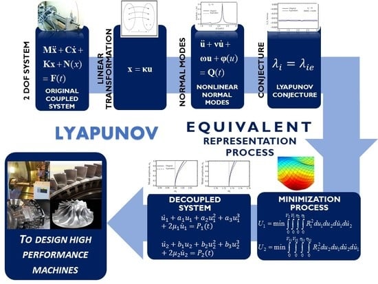
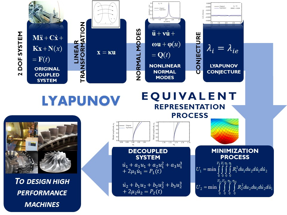
2. Transformation Technique

Before the decoupling procedure to find the equivalent representation form of Equation (1) in the sense of Lyapunov is introduced, Equation (1) is first written into its canonical, normal mode by applying the following linear transformation [36]

$$\left\{\begin{array}{c}{x}_1\\ x_2\end{array}\right\}=\mathit{\kappa }\left\{\begin{array}{c}{u}_1\\ u_2\end{array}\right\}$$

(3)

which yields:

$$\begin{array}{c}\left[\begin{array}{cc}1& 0\\ 0& 1\end{array}\right]\left\{\begin{array}{c}{\ddot{u}}_1\\ {\ddot{u}}_2\end{array}\right\}+\left[\begin{array}{cc}{\nu }_1& {\nu }_2\\ {\nu }_2& {\nu }_3\end{array}\right]\left\{\begin{array}{c}{\dot{u}}_1\\ {\dot{u}}_2\end{array}\right\}+\left[\begin{array}{cc}{\omega }_{n1}^2& 0\\ 0& {\omega }_{n2}^2\end{array}\right]\left\{\begin{array}{c}{u}_1\\ u_2\end{array}\right\}\\ +\left\{\begin{array}{c}{\phi }_1{u}_1^3+{\phi }_2{u}_1^2{u}_2+{\phi }_3{u}_1{u}_2^2+{\phi }_4{u}_2^3\\ {\phi }_5{u}_1^3+{\phi }_6{u}_1^2{u}_2+{\phi }_7{u}_1{u}_2^2+{\phi }_8{u}_2^3\end{array}\right\}=\left\{\begin{array}{c}{P}_1\left(t\right)\\ P_2\left(t\right)\end{array}\right\}\end{array}$$

(4)

where $u_1$ and $u_2$ are the normal coordinates of the linear, undamped, free vibration system, $\mathit{\kappa }$ is the modal matrix which consists of the characteristic vectors that represent the natural modes of the linear system obtained from (1), and these are given by $\mathit{\kappa }=\left[R_1{\left\{\kappa \right\}}_1,R_2{\left\{\kappa \right\}}_2\right]$, where $R_i$ are scale factors that can be determined from $\sqrt{1/M_{ii}}$, in which $M_{ii}={\mathit{\kappa }}_i^T\mathit{M}{\mathit{\kappa }}_i$ is the generalized mass and ${\left\{\kappa \right\}}_1$ and ${\left\{\kappa \right\}}_2$ denote column eigenvectors. If the scale factors are chosen so that $M_{ii}={\mathit{\kappa }}_i^T\mathit{M}{\mathit{\kappa }}_i=1,$ $i=1,2$, then the normal modes are mass-orthonormal, and thus, ${\omega }_{ni}^2={\mathit{\kappa }}_i^T\mathit{M}{\mathit{\kappa }}_i,$ $i=1,2$. Furthermore, ${\phi }_1$ through ${\phi }_8$, and $P_1\left(t\right)$ and $P_2\left(t\right)$ are parameters that are defined in accordance with the physics of the system. Here, the initial conditions are assumed to be given as $u_1\left(0\right)=u_{10}$, $u_2\left(0\right)=u_{20}$, ${\dot{u}}_1\left(0\right)={\dot{u}}_{10}$ and ${\dot{u}}_2\left(0\right)={\dot{u}}_{20}$. It is further assumed that the linear transformation (3) preserves the Lyapunov exponents of the original system (1); this implies that Lyapunov exponents of the original system (1) are equal to those computed from (4) and hold for any solution of the original system and the corresponding solution of the transformed one, as stated by Barabanov [37].

On the other hand, one can notice that the nonlinear Equation (4) does not have known exact solutions and is as difficult to solve as the original equations of motion (1). In order to avoid these difficulties, it is now assumed that the modal system (4) can be expressed, for the system generalized coordinates (displacements or rotations), in a third-order power series expansion [18,19,20,21]. Thus, Equation (4) becomes

$$\begin{array}{r}{\ddot{u}}_1+{\omega }_{n1}^2{u}_1+{\nu }_1{\dot{u}}_1+{\nu }_2{\dot{u}}_2+{\phi }_1{u}_1^3+{\phi }_2{u}_1^2{u}_2+{\phi }_3{u}_1{u}_2^2+{\phi }_4{u}_2^3\\ \equiv {\ddot{u}}_1+a_1{u}_1+a_2{u}_1^2+a_3{u}_1^3+2{\mu }_1{\dot{u}}_1+\cdots =P_1\left(t\right)\end{array}$$

(5)

$$\begin{array}{r}{\ddot{u}}_2+{\omega }_{n2}^2{u}_2+{\nu }_2{\dot{u}}_1+{\nu }_3{\dot{u}}_2+{\phi }_5{u}_1^3+{\phi }_6{u}_1^2{u}_2+{\phi }_7{u}_1{u}_2^2+{\phi }_8{u}_2^3\\ \equiv {\ddot{u}}_2+b_1{u}_2+b_2{u}_2^2+b_3{u}_2^3+2{\mu }_2{\dot{u}}_2+\cdots =P_2\left(t\right)\end{array}$$

(6)

Expressions (5) and (6) provide approximate decoupled representation forms of the original equations of motion whose accuracy depends on the unknown coefficients: $a_i$, $b_i$, and ${\mu }_i$. Here, the external forces and the driving frequencies are considered to be the same in both systems [16,38]. Once these coefficients are determined, the approximate solutions of (5) and (6) can be derived by using perturbation or numerical techniques [39], and their LCEs can be numerically computed by using the procedure discussed in [40,41].

The following remarks are important to set the number of terms of the power series expansion of Equations (5) and (6) that provides an invariant polynomial expression which describes the shapes of the invariant manifolds that are related to the system’s nonlinear normal modes [21,38,42]:

(a)

Odd terms arise in the right-hand term (RHT) of the invariant polynomial expressions of Equations (5) and (6) if the restoring forces of the dynamic system are described by an invariant odd polynomial expression.

(b)

If the restoring forces of the original system have mixed-parity nonlinearities, then even and odd terms arise in the RHT invariant polynomial expressions of Equations (5) and (6).

(c)

Velocity-dependent terms arise mainly in the RHT of the invariant polynomial expressions of Equations (5) and (6) in order to capture not only the effective trend of the system’s nonlinearities responsible for displaying amplitude-dependent nonlinear mode shapes, but also to take into account decay rate effects.

3. Determination of $a_i$, $b_i$, and ${\mu }_i$

To determine the coefficients $a_i$, $b_i$, and ${\mu }_i$, a minimization procedure analogous to the one followed by Caughley in [2] is assumed. Here, it is assumed that the square of the difference between the acceleration of the originally coupled system and that of the simplified cubic one, given by Expressions (5) and (6), could be minimized for each system by considering that the weighted mean square errors, U₁ and U₂, can be determined by using the following expressions [17]:

$$\begin{array}{c}{U}_1=\min \underset{0}{\overset{V_2}{{\displaystyle \int }}}\underset{0}{\overset{V_1}{{\displaystyle \int }}}\underset{0}{\overset{{\eta }_2}{{\displaystyle \int }}}\underset{0}{\overset{{\eta }_1}{{\displaystyle \int }}}({\omega }_{n1}^2{u}_1+{\nu }_1{\dot{u}}_1+{\nu }_2{\dot{u}}_2+{\phi }_1{u}_1^3+{\phi }_2{u}_1^2{u}_2+{\phi }_3{u}_1{u}_2^2+{\phi }_4{u}_2^3-a_1{u}_1\\ -a_2{u}_1^2-a_3{u}_1^3-2{\mu }_1{\dot{u}}_1-\cdots ){}^2 d{u}_1 d{u}_2 d{\dot{u}}_1 d{\dot{u}}_2,\end{array}$$

(7)

$$\begin{array}{c}{U}_2=\min \underset{0}{\overset{V_{11}}{{\displaystyle \int }}}\underset{0}{\overset{V_{22}}{{\displaystyle \int }}}\underset{0}{\overset{{\eta }_{11}}{{\displaystyle \int }}}\underset{0}{\overset{{\eta }_{22}}{{\displaystyle \int }}}({\omega }_{n2}^2{u}_2+2{\nu }_2{\dot{u}}_1+{\nu }_3{\dot{u}}_2+{\phi }_5{u}_1^3+{\phi }_6{u}_1^2{u}_2+{\phi }_7{u}_1{u}_2^2+{\phi }_8{u}_2^3\\ -b_1{u}_2-b_2{u}_2^2-b_3{u}_2^3-2{\mu }_2{\dot{u}}_2-\cdots ){}^2 d{u}_2 d{u}_1 d{\dot{u}}_2 d{\dot{u}}_1.\end{array}$$

(8)

Furthermore, the minimization of $U_1$ and $U_2$ with respect to the coefficients, a_i, b_i and μ_i, can be achieved from [9]

$$\frac{\partial U_1}{\partial a_i}=0\mathrm{with} i=1, 2, 3,\frac{\partial U_1}{\partial {\mu }_1}=0,$$

(9)

$$\frac{\partial U_2}{\partial b_i}=0\mathrm{with} i=1, 2, 3,\frac{\partial U_2}{\partial {\mu }_2}=0.$$

(10)

Equations (9) and (10) yield, after performing some algebraic computer calculations with the help of Mathematica 11.1.1.0 symbolic computer package, the following expressions:

$$a_1={\omega }_{n1}^2+\frac{{\phi }_3{\eta }_2^2}{3}+\frac{85}{74{\eta }_1}\left({\phi }_4{\eta }_2^3+2{\nu }_2{V}_2\right),a_2=\frac{37{\phi }_2{\eta }_1^2{\eta }_2-320\left({\phi }_4{\eta }_2^3+{\nu }_2{V}_2\right)}{37{\eta }_1^2},$$

(11)

$$a_3=\frac{111{\phi }_1{\eta }_1^3+560\left({\phi }_4{\eta }_2^3+{\nu }_2{V}_2\right)}{111{\eta }_1^3},{\mu }_1=\frac{48{\phi }_4{\eta }_2^3+37{\nu }_1{V}_1+48{\nu }_2{V}_2}{74V_1},$$

(12)

$$b_1=-\frac{-222{\eta }_{22}{\omega }_{n2}^2-255{\phi }_5{\eta }_{11}^3-74{\phi }_6{\eta }_{11}^2{\eta }_{22}-510{\nu }_2{V}_{11}}{222{\eta }_{22}},$$

(13)

$$b_2=-\frac{160{\phi }_5{\eta }_{11}^3-37{\phi }_7{\eta }_{11}{\eta }_{22}^2+320{\nu }_2{V}_{11}}{74{\eta }_{22}^2},$$

(14)

$$b_3=-\frac{-140{\phi }_5{\eta }_{11}^3-111{\phi }_8{\eta }_{22}^3-280{\nu }_2{V}_{11}}{111{\eta }_{22}^2},$$

(15)

$${\mu }_2=-\frac{-12{\phi }_5{\eta }_{11}^3-24{\nu }_2{V}_{11}-37{\nu }_3{V}_{22}}{74V_{22}}.$$

(16)

Here, ${\eta }_i$, ${\eta }_{ii}$, $V_i$, and $V_{ii}$ describe integration constants whose values must minimize Expressions (7) and (8). The general procedure to compute the integration constants ${\eta }_i$, ${\eta }_{ii}$, $V_i$, and $V_{ii}$ is discussed in the following section.

Computation of ${\eta }_i$, ${\eta }_{ii}$, $V_i$, and $V_{ii}$ Values

To determine the above integration constants, Equations (11) and (12) are substituted into Equations (7), and (13)–(16) are substituted into Equation (8). This step yields, after performing the corresponding integrations, the following expressions:

$$S_1=\frac{121{\eta }_1{\eta }_2{V}_1{V}_2}{258741}\left(12{\phi }_4^2{\eta }_2^6+21{\phi }_4{\eta }_2^3{\nu }_2{V}_2+28{\nu }_2^2{V}_2^2\right),$$

(17)

$$\begin{array}{ll}{S}_2=\frac{{\eta }_{11}{\eta }_{22}{V}_{11}{V}_{22}}{41398560}& (3780750{\phi }_5^2{\eta }_{11}^6+3677800{\phi }_5{\phi }_6{\eta }_{11}^5{\eta }_{22}+1226624{\phi }_6^2{\eta }_{11}^4{\eta }_{22}^2\\ & +2206680{\phi }_5{\phi }_7{\eta }_{11}^4{\eta }_{22}^2+1724940{\phi }_6{\phi }_7{\eta }_{11}^3{\eta }_{22}^3+689976{\phi }_7^2{\eta }_{11}^2{\eta }_{22}^4\\ & +4957575{\phi }_5{\nu }_2{\eta }_{11}^3{V}_{11}+2755760{\phi }_6{\nu }_2{\eta }_{11}^2{\eta }_{22}{V}_{11}+2066820{\phi }_7{\nu }_2{\eta }_{11}{\eta }_{22}^2{V}_{11}\\ & +4952920{\nu }_2^2{V}_{11}^2),\end{array}$$

(18)

Notice that the resulting polynomial expressions, (17) and (18), provide convex, continuous functions in the relative interior of their domains which depend on the values of ${\eta }_i$, ${\eta }_{ii}$, $V_i$, and $V_{ii}$ [43,44]. These functions, $S_i$, have a unique minimum value within their bounded domain intervals, as discussed in [45,46] and references cited therein. Thus, the values of ${\eta }_i$, ${\eta }_{ii}$, $V_i$, and $V_{ii}$ that provide the minimum values of $U_i$ could be computed by following a classical minimization algorithm in which the partial derivatives of Equations (17) and (18) must be determined, respectively, with respect to the unknowns: ${\eta }_i$, ${\eta }_{ii}$, $V_i$, and $V_{ii}$. This step provides the following equations:

$$\frac{\partial S_1}{\partial {\eta }_1}=\frac{121{\eta }_2{V}_1{V}_2}{258741}\left(12{\phi }_4^2{\eta }_2^6+21{\phi }_4{\eta }_2^3{\nu }_2{V}_2+28{\nu }_2^2{V}_2^2\right),$$

(19)

$$\frac{\partial S_1}{\partial {\eta }_2}=\frac{484{\eta }_1{V}_1{V}_2}{369663}\left(3{\phi }_4^2{\eta }_2^6+3{\phi }_4{\eta }_2^3{\nu }_2{V}_2+{\nu }_2^2{V}_2^2\right),$$

(20)

$$\frac{\partial S_1}{\partial V_1}=\frac{121{\eta }_1{\eta }_2{V}_2}{258741}\left(12{\phi }_4^2{\eta }_2^6+21{\phi }_4{\eta }_2^3{\nu }_2{V}_2+28{\nu }_2^2{V}_2^2\right),$$

(21)

$$\frac{\partial S_1}{\partial V_2}=\frac{242{\eta }_1{\eta }_2{V}_1}{86247}\left(2{\phi }_4^2{\eta }_2^6+7{\phi }_4{\eta }_2^3{\nu }_2{V}_2+14{\nu }_2^2{V}_2^2\right),$$

(22)

$$\begin{array}{ll}\frac{\partial S_2}{\partial {\eta }_{11}}=\frac{{\eta }_{22}{V}_{11}{V}_{22}}{2957040}& (1890375{\phi }_5^2{\eta }_{11}^6+1576200{\phi }_5{\phi }_6{\eta }_{11}^5{\eta }_{22}+438080{\phi }_6^2{\eta }_{11}^4{\eta }_{22}^2\\ & +788100{\phi }_5{\phi }_7{\eta }_{11}^4{\eta }_{22}^2+492840{\phi }_6{\phi }_7{\eta }_{11}^3{\eta }_{22}^3+147852{\phi }_7^2{\eta }_{11}^2{\eta }_{22}^4\\ & +1416450{\phi }_5{\nu }_2{\eta }_{11}^3{V}_{11}+590520{\phi }_6{\nu }_2{\eta }_{11}^2{\eta }_{22}{V}_{11}+295260{\phi }_7{\nu }_2{\eta }_{11}{\eta }_{22}^2{V}_{11}\\ & +353780{\nu }_2^2{V}_{11}^2),\end{array}$$

(23)

$$\begin{array}{ll}\frac{\partial S_2}{\partial {\eta }_{22}}=\frac{{\eta }_{11}{V}_{11}{V}_{22}}{41398560}& (3780750{\phi }_5^2{\eta }_{11}^6+7355600{\phi }_5{\phi }_6{\eta }_{11}^5{\eta }_{22}+3679872{\phi }_6^2{\eta }_{11}^4{\eta }_{22}^2\\ & +6620040{\phi }_5{\phi }_7{\eta }_{11}^4{\eta }_{22}^2+6899760{\phi }_6{\phi }_7{\eta }_{11}^3{\eta }_{22}^3+3449880{\phi }_7^2{\eta }_{11}^2{\eta }_{22}^4\\ & +4957575{\phi }_5{\nu }_2{\eta }_{11}^3{V}_{11}+5511520{\phi }_6{\nu }_2{\eta }_{11}^2{\eta }_{22}{V}_{11}+6200460{\phi }_7{\nu }_2{\eta }_{11}{\eta }_{22}^2{V}_{11}\\ & +4952920{\nu }_2^2{V}_{11}^2),\end{array}$$

(24)

$$\begin{array}{ll}\frac{\partial S_2}{\partial V_{11}}=\frac{{\eta }_{11}{\eta }_{22}{V}_{22}}{20699280}& (1890375{\phi }_5^2{\eta }_{11}^6+1838900{\phi }_5{\phi }_6{\eta }_{11}^5{\eta }_{22}+613312{\phi }_6^2{\eta }_{11}^4{\eta }_{22}^2\\ & +1103340{\phi }_5{\phi }_7{\eta }_{11}^4{\eta }_{22}^2+862470{\phi }_6{\phi }_7{\eta }_{11}^3{\eta }_{22}^3+344988{\phi }_7^2{\eta }_{11}^2{\eta }_{22}^4\\ & +4957575{\phi }_5{\nu }_2{\eta }_{11}^3{V}_{11}+2755760{\phi }_6{\nu }_2{\eta }_{11}^2{\eta }_{22}{V}_{11}+2066820{\phi }_7{\nu }_2{\eta }_{11}{\eta }_{22}^2{V}_{11}\\ & +7429380{\nu }_2^2{V}_{11}^2),\end{array}$$

(25)

$$\begin{array}{ll}\frac{\partial S_2}{\partial V_{22}}=\frac{{\eta }_{11}{\eta }_{22}{V}_{11}}{41398560}& (3780750{\phi }_5^2{\eta }_{11}^6+3677800{\phi }_5{\phi }_6{\eta }_{11}^5{\eta }_{22}+1226624{\phi }_6^2{\eta }_{11}^4{\eta }_{22}^2\\ & +2206680{\phi }_5{\phi }_7{\eta }_{11}^4{\eta }_{22}^2+1724940{\phi }_6{\phi }_7{\eta }_{11}^3{\eta }_{22}^3+689976{\phi }_7^2{\eta }_{11}^2{\eta }_{22}^4\\ & +4957575{\phi }_5{\nu }_2{\eta }_{11}^3{V}_{11}+2755760{\phi }_6{\nu }_2{\eta }_{11}^2{\eta }_{22}{V}_{11}+2066820{\phi }_7{\nu }_2{\eta }_{11}{\eta }_{22}^2{V}_{11}\\ & +4952920{\nu }_2^2{V}_{11}^2),\end{array}$$

(26)

which are set equal to zero to find the critical points at which Equations (7) and (8) are minimized. Notice from Equation (9) through (16) that the denominator terms depend, respectively, on ${\eta }_1$, $V_1$, ${\eta }_{22}$, and $V_{22}$. Therefore, these coefficients cannot be zero. Thus, $\partial S_1/\partial {\eta }_1=0$, $\partial S_1/\partial {\eta }_2=0$, $\partial S_1/\partial V_1=0$, $\partial S_1/\partial V_2=0$, $\partial S_2/\partial {\eta }_{11}=0$, $\partial S_2/\partial {\eta }_{22}=0$, $\partial S_2/\partial V_{11}=0$, $\partial S_2/\partial V_{22}=0$ are identically satisfied, if, and only if, ${\eta }_2=0$, $V_2=0$, ${\eta }_{11}=0$, and $V_{11}=0$. Then, the expressions for $a_i$ and $b_i$ that minimize the weighted mean square error of using Expressions (7) and (8) to determine the coefficients, $a_i$, $b_i$, and ${\mu }_i$ that describes the equivalent representation form of the original equation of motion, into the approximate forms (5) and (6), simplify to

$$a_1={\omega }_{n1}^2,a_2=0,a_3={\phi }_1,{\mu }_1=\frac{{\nu }_1}{2},$$

(27)

$$b_1={\omega }_{n2}^2,b_2=0,b_3={\phi }_8,{\mu }_2=\frac{{\nu }_3}{2}.$$

(28)

Thus, the above approach and the usage of power series expansion up to the third-order to replace the modal restoring forces of Equations (5) and (6) provide the following uncoupled Duffing-type equivalent equations:

$${\ddot{u}}_1+2{\mu }_1{\dot{u}}_1+a_1{u}_1+a_3{u}_1^3=P_1\left(t\right),{\ddot{u}}_2+2{\mu }_2{\dot{u}}_2+b_1{u}_2+b_3{u}_2^3=P_2\left(t\right).$$

(29)

It is important to point out that such equivalence in this two degree-of-freedom (DOF), non-integrable system (4) is only equivalent, in an approximate form, to two single degree-of-freedom integrable equations. Furthermore, in the conservative case, almost periodic solutions can be observed in two-DOF nonlinear system of coupled equations, but they are absent in the uncoupled, single-DOF, nonlinear Equation (29). However, the linear combination of their approximate solutions, in accordance with Equation (3), could exhibit, as in the case of the original system of differential Equation (1), almost periodic solutions, as will be demonstrated in Example 2. In accordance with Shaw and Pierre [20], the advantage of having decoupled modal equations is related to the possibility of obtaining information about the system modal amplitudes and thus, the numerical integration solution of these equivalent expressions, which could provide valuable information about the qualitative and quantitative behaviors of the system dynamics.

On the other hand, if the restoring forces, $f_1\left(x_1,x_2\right)$ and $f_2\left(x_1,x_2\right),$ of the dynamic system (1) contain even, nonlinear effects, then, their equivalent representation forms in the sense of Lyapunov could also be expanded to power series in which decay terms must be considered. Section 5 focuses on studying the effects of these new terms in the decoupled form of a nonlinear, dynamic system.

4. Numerical Validation

The applicability of the proposed approach of replacing, in the sense of Lyapunov, a two-degree-of-freedom system with equivalent expressions of the Duffing type will be examined by considering three nonlinear dynamic systems.

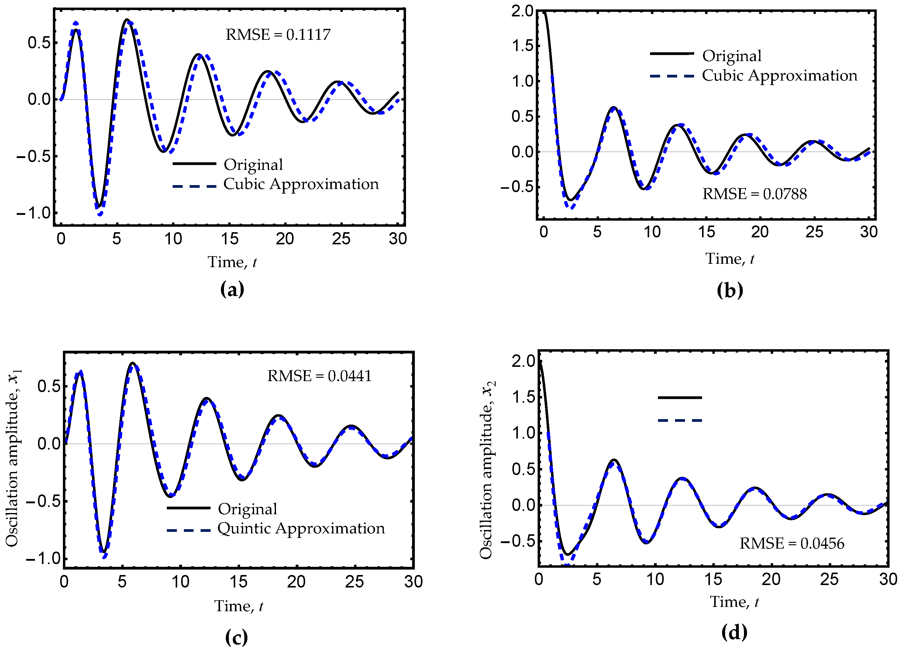
4.1. Example 1: Dynamic System with Cubic Nonlinearities

To study the accuracy attained by applying the proposed approach to decouple nonlinear differential equations and to validate the proposed conjecture, first, the frequency-amplitude response curves of the original unforced, undamped system (4) will be compared to the backbone curves obtained from the Duffing equations described by Equation (29). To accomplish this goal, the nonlinear dynamic systems discussed in [20,21] are considered, in which the corresponding equations of motion are described by

$$\left[\begin{array}{cc}m& 0\\ 0& m\end{array}\right]\left\{\begin{array}{c}{\ddot{x}}_1\\ {\ddot{x}}_2\end{array}\right\}+\left[\begin{array}{cc}c& -c\\ -c& 2c\end{array}\right]\left\{\begin{array}{c}{\dot{x}}_1\\ {\dot{x}}_2\end{array}\right\}+\left[\begin{array}{cc}1+k& -k\\ -k& 1+k\end{array}\right]\left\{\begin{array}{c}{x}_1\\ x_2\end{array}\right\}+\left\{\begin{array}{c}\epsilon x_1^3\\ 0\end{array}\right\}=\left\{\begin{array}{c}{f}_1\cos {\omega }_{f}t\\ 0\end{array}\right\}$$

(30)

where $f_1$ is the magnitude of the driving force, and ${\omega }_f$ represents the corresponding driving frequency. The system initial conditions are assumed to be given as $x_1\left(0\right)=x_{10}$, ${\dot{x}}_1\left(0\right)=0$, $x_2\left(0\right)=x_{20}$, and ${\dot{x}}_2\left(0\right)=0$. In order to study the dynamic response of the system (30), this is first transformed into the modal coordinates, ${\left\{\begin{array}{cc}{u}_1& u_2\end{array}\right\}}^T$, via the following linear transformation

$$\left\{\begin{array}{c}{x}_1\\ x_2\end{array}\right\}=\left[\begin{array}{cc}\beta & \beta \\ \beta & -\beta \end{array}\right]\left\{\begin{array}{c}{u}_1\\ u_2\end{array}\right\}$$

(31)

where $\beta =1/\sqrt{2}$. Thus, the system (30) can be equivalently written as Equation (4) with

$$\begin{array}{c}{\phi }_1\equiv \epsilon /8,{\phi }_2\equiv -3\epsilon /8,{\phi }_3\equiv 3\epsilon /8,{\phi }_4\equiv -\epsilon /8,{\phi }_5\equiv -\epsilon /8,{\phi }_6\equiv 3\epsilon /8,\\ {\phi }_7\equiv -3\epsilon /8,{\phi }_8\equiv \epsilon /8,{\nu }_1={\nu }_2=1/2c,{\nu }_3\equiv 5/2c,{\omega }_{n1}^2\equiv 1/m, \\ {\omega }_{n2}^2=\left(1+2k\right)/m,P_1\left(t\right)=P_2\left(t\right)=f_1/\sqrt{2}\cos {\omega }_{f}t.\end{array}$$

(32)

In order to determine if the decoupled Equation (29) provides a good description of the dynamics of the original system (30), the frequency-amplitude backbone curves are plotted. In accordance with Hsu [47], the exact frequency-amplitude equations for the unforced, undamped Duffing Equation (4) are given as

$$\mathrm{mode}1:{\omega }_1^2=a_1+a_3{u}_{10}^2;\mathrm{mode}2:{\omega }_2^2=b_1+b_3{u}_{20}^2$$

(33)

while the approximate frequency-amplitude relationships obtained from the modified Lindstedt–Poincaré method are [48,49]

$$\mathrm{mode}1:{\omega }_1^2={\omega }_{n1}^2+1/4\left(3/8\epsilon u_{10}^2+3/8\epsilon u_{10}{u}_{20}+O\left({\epsilon }^2\right)\right),$$

(34)

$$\mathrm{mode}2:{\omega }_2^2={\omega }_{n2}^2+1/4\left(3/8\epsilon u_{20}^2+3/8\epsilon u_{10}{u}_{20}+O\left({\epsilon }^2\right)\right).$$

(35)

Figure 1 shows the simulation performed to verify the accuracy of the proposed methodology that decouples the nonlinear normal mode’s differential equations. The system parameter values in dimensionless units are $m=1$, $k=1$, $\epsilon =0.5$ with $c=0$ and $f_1=0$; these are similar to those used in [20]. To plot the frequency-amplitude curve of the first mode, initial conditions of $\left(u_1, u_2, {\dot{u}}_1, {\dot{u}}_2\right)=\left(1, 0, 0, 0\right)$ were considered, and for the second mode, $\left(u_1, u_2, {\dot{u}}_1, {\dot{u}}_2\right)=\left(0, 1, 0, 0\right)$ was used. It is clear from the results exhibited in Figure 1 that the frequency-amplitude curves of the original system compare well with those of the uncoupled equations. Therefore, it is concluded that the replacement of the original equation of motion for two equivalent equations of the Duffing-type describes the qualitative and quantitative dynamic system behaviors well, as shown in Figure 2, in which the frequency-amplitude backbone curves for several values of $k$ and $\epsilon$ have been plotted.

Next, the damped nonlinear case was considered with parameter values of $m=1$, $c=0.3$, $k=1$ and $\epsilon =0.5$ to compare the numerical integration of Equation (30) with respect to those given by expressions (29). The results of the simulations in physical coordinates are depicted in Figure 3 in which the amplitude-time curves have been plotted by using the system’s initial conditions of $\left(x_1, x_2, {\dot{x}}_1, {\dot{x}}_2\right)=\left(0, 0, 2, 0\right)$.

It is evident from Figure 3, that the decoupled Equation (29) is in agreement with the numerical integration solutions of the original equations of motion (30). In fact, the LCEs of the original system have mean values of ${\lambda }_1=-0.0756$, ${\lambda }_2=-0.0802$, ${\lambda }_3=-0.3698$, and ${\lambda }_4=-0.3743$ bits/second, while the LCEs computed from the equivalent models are ${\lambda }_{1e}=-0.0749$, ${\lambda }_{2e}=-0.0750$, ${\lambda }_{3e}=-0.3726$, and ${\lambda }_{4e}=-0.3773$ bits/second. In spite of having some discrepancies in the computed numerical values, the order of magnitude of the LCEs of the equivalent expressions tend to be similar to those computed from the original equations of motion with root mean square error (RMSE) values of 0.1117 and 0.0788 for the first and second mode, respectively.

To further assess the accuracy of the proposed nonlinear decoupling procedure, the frequency-amplitude steady-state response curves of the forced, damped nonlinear system (30) were plotted with parameter values of $m=1$, $k=1$, $c=0.3$, $\epsilon =0.5$ and $f_1=0.25$.

It can be seen from Figure 4 that the numerical integration solutions of the decoupled Equation (29) provide curves that slightly differ close to the resonant region to those obtained from the numerical integration solutions of the original equations of motion, but its qualitative and quantitative system dynamic predictions are, in general, good. The corresponding Largest Lyapunov Characteristic Exponent (LLE) curves plotted versus the driving frequency, ${\omega }_f$, are exhibited in Figure 5. It is evident from Figure 5 that the LLE curve computed from the equivalent uncoupled expressions (29) is closed to that estimated from Equation (30). In this case, the RMSE does not exceed the value of 0.0056. This confirms that the proposed conjecture is numerically true.

As a second example to investigate the validity of the proposed conjecture, a forced, damped nonlinear dynamic system with cubic nonlinearities was next examined.

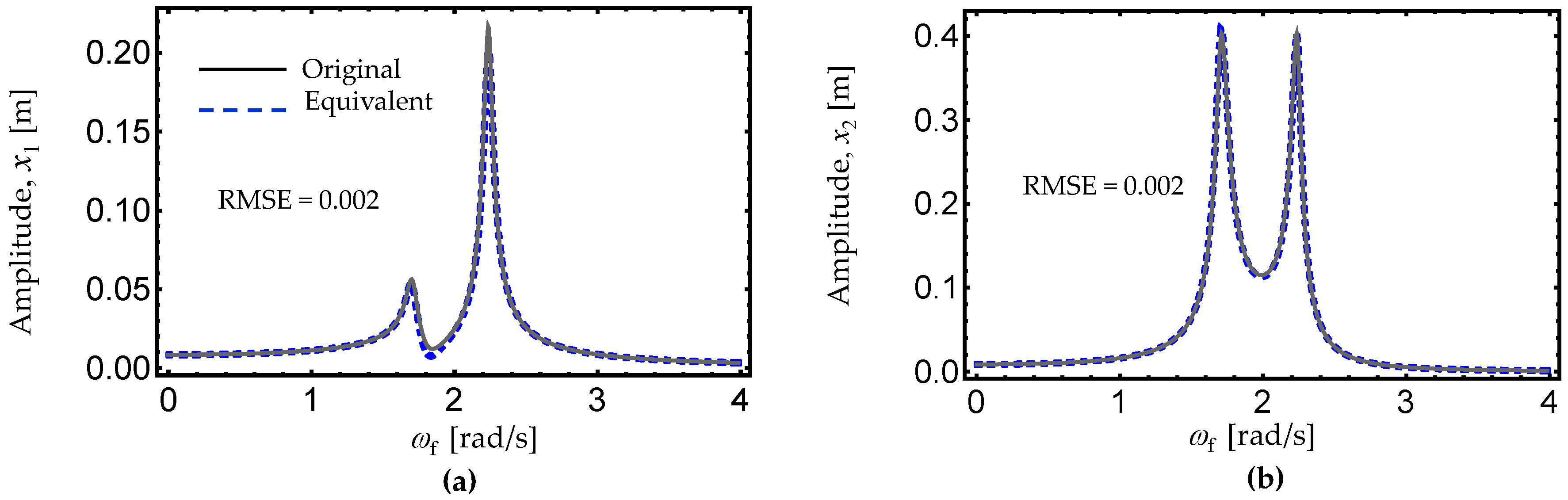
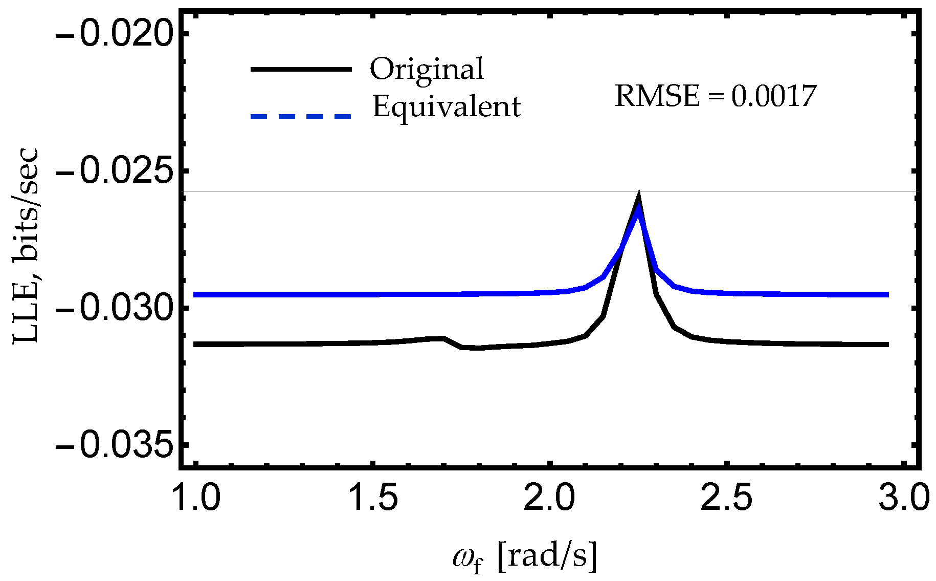
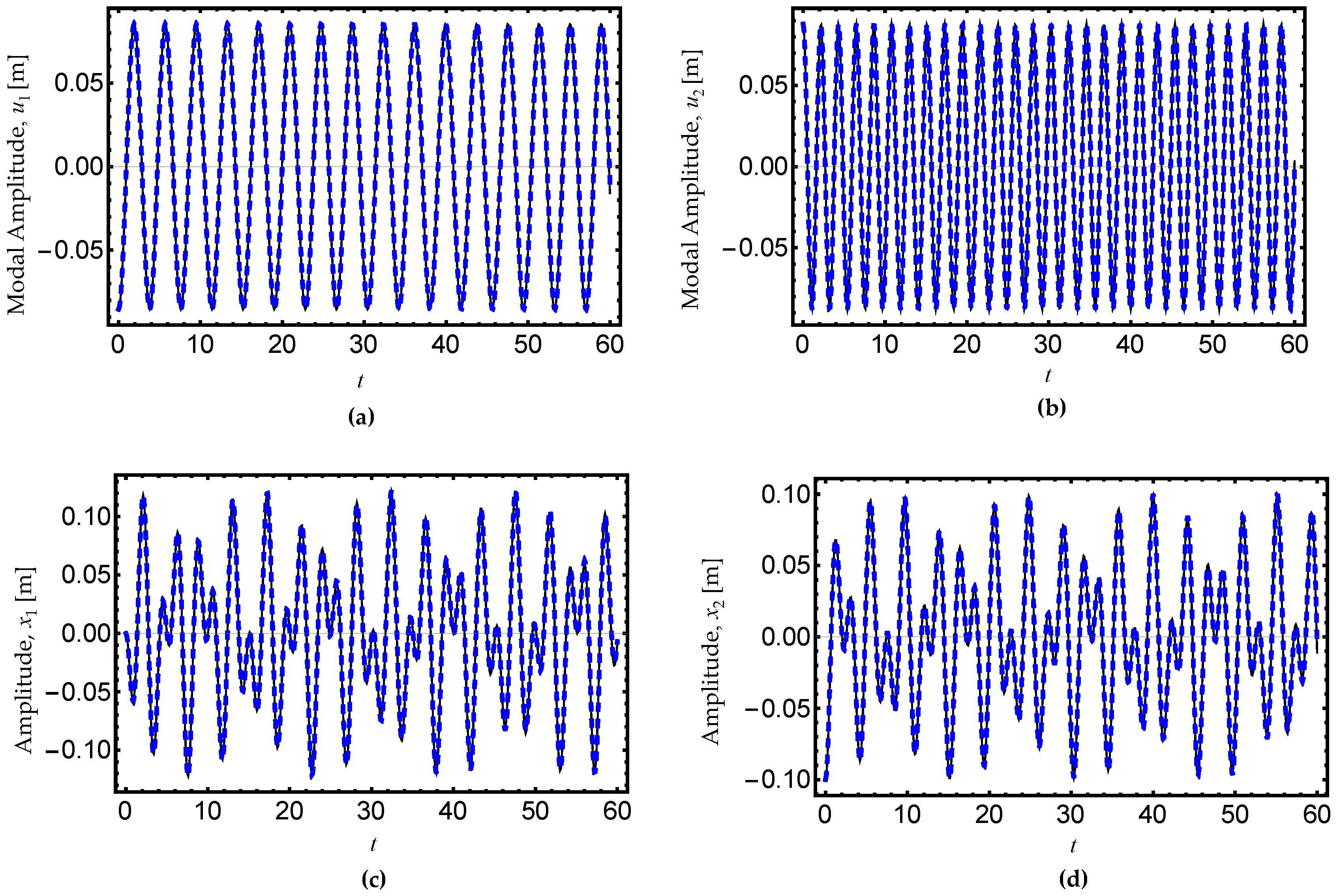
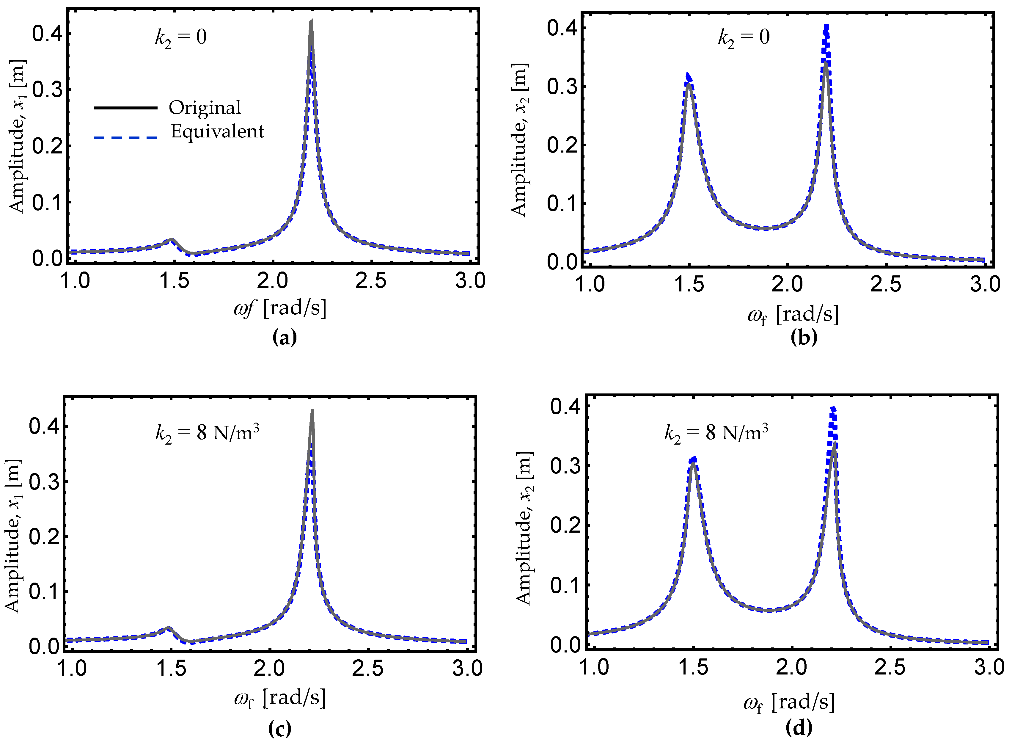
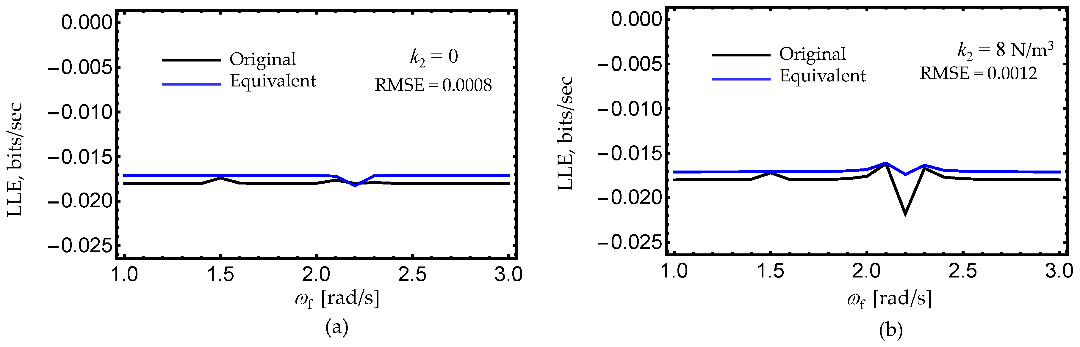
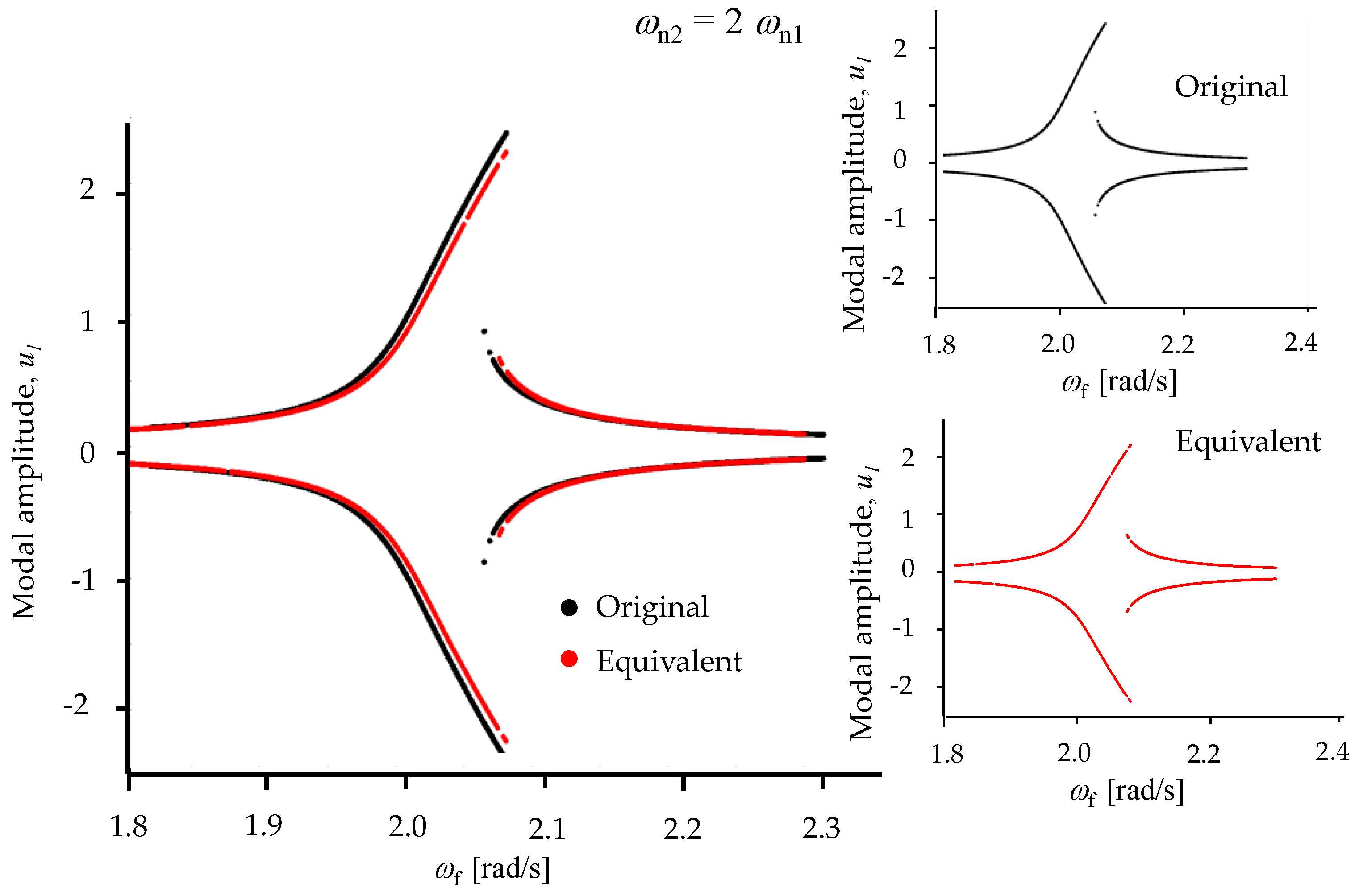
4.2. Example 2: A Forced System with Cubic Nonlinearities

Here, the nonlinear dynamic system introduced in [21] was examined, which has the form

$$\left[\begin{array}{cc}{m}_1& 0\\ 0& m_2\end{array}\right]\left\{\begin{array}{c}{\ddot{x}}_1\\ {\ddot{x}}_2\end{array}\right\}+\left[\begin{array}{cc}{c}_1& 0\\ 0& c_2\end{array}\right]\left\{\begin{array}{c}{\dot{x}}_1\\ {\dot{x}}_2\end{array}\right\}+\left[\begin{array}{cc}{k}_1+k_2& -k_2\\ -k_2& k_2+k_3\end{array}\right]\left\{\begin{array}{c}{x}_1\\ x_2\end{array}\right\}+\left\{\begin{array}{c}{\epsilon }_1{x}_1^3\\ {\epsilon }_2{x}_2^3\end{array}\right\}=\left\{\begin{array}{c}{Q}_1\cos {\omega }_{f}t\\ 0\end{array}\right\},$$

(36)

with initial conditions given by $x_1\left(0\right)=x_{10}$, ${\dot{x}}_1\left(0\right)=0$, $x_2\left(0\right)=x_{20}$, and ${\dot{x}}_2\left(0\right)=0$. To find the canonical representation form of Equation (36), the following transformation approach is applied [36]:

$$\left\{\begin{array}{c}{x}_1\\ x_2\end{array}\right\}=\left[\begin{array}{cc}{R}_1& R_2\\ R_1{f}_1& R_2{f}_2\end{array}\right]\left\{\begin{array}{c}{u}_1\\ u_2\end{array}\right\},$$

(37)

which yields the canonical form (4). In this case,

$${\omega }_{n1}^2=\frac{1}{2m_1{m}_2}\left[k_1{m}_2+k_2\left(m_1+m_2\right)+k_3{m}_1-H_1\right],$$

(38)

$${\omega }_{n2}^2=\frac{1}{2m_1{m}_2}\left[k_1{m}_2+k_2\left(m_1+m_2\right)+k_3{m}_1+H_1\right],$$

(39)

where

$$H_1=\sqrt{{\left(\left(k_2+k_3\right)m_1+k_1+k_2{m}_2\right)}^2-4\left(k_2{k}_3+k_1\left(k_2+k_3\right)\right)m_1{m}_2}$$

(40)

and

$$\begin{array}{c}{\nu }_1=\left(c_1+c_2{f}_1^2\right)r_1^2,{\nu }_2=\left(c_1+c_2{f}_1{f}_2\right)r_1{r}_2,{\nu }_3=\left(c_1+c_2{f}_2^2\right)r_2^2,\\ {\phi }_1\equiv {\epsilon }_1{R}_1^4+f_1^4{\epsilon }_2{R}_1^4,{\phi }_2\equiv 3R_1^3{R}_2{\epsilon }_1+3f_1^3{f}_2{\epsilon }_2{R}_1^3{R}_2,{\phi }_3\equiv 3R_1^2{R}_2^2{\epsilon }_1+3f_1^2{f}_2^2{\epsilon }_2{R}_1^2{R}_2^2,\\ {\phi }_4\equiv R_1{R}_2^3{\epsilon }_1+f_1{f}_2^3{\epsilon }_2{R}_1{R}_2^3,{\phi }_5\equiv R_1^3{R}_2{\epsilon }_1+f_1^3{f}_2{\epsilon }_2{R}_1^3{R}_2,{\phi }_6\equiv 3R_1^2{R}_2^2{\epsilon }_1+3f_1^2{f}_2^2{\epsilon }_2{R}_1^2{R}_2^2,\\ {\phi }_7\equiv 3R_1{R}_2^3{\epsilon }_1+f_1{f}_2^3{\epsilon }_2{R}_1{R}_2^3,{\phi }_8\equiv R_2^4{\epsilon }_1+f_2^4{\epsilon }_2{R}_2^4,\\ f_1\equiv \frac{k_1+k_2-m_1{\omega }_{n1}^2}{k_2},f_2\equiv \frac{k_1+k_2-m_1{\omega }_{n2}^2}{k_2},P_1\left(t\right)\equiv R_1{Q}_1\cos {\omega }_{f}t.\end{array}$$

(41)

Thus, the equivalent decoupled representation form of Equation (36), becomes

$${\ddot{u}}_1+2{\mu }_1{\dot{u}}_1+a_1{u}_1+a_3{u}_1^3=P_1\left(t\right),{\ddot{u}}_2+2{\mu }_2{\dot{u}}_2+b_1{u}_2+b_3{u}_2^3=P_2\left(t\right).$$

(42)

where $a_i$, $b_i$, and ${\mu }_i$, are defined by Equations (27) and (28).

To assess the precision of the proposed approach, the frequency amplitude response curves were next computed using the following system parameter values: $m_1=1$ kg, $m_2=1.5$ kg, $k_1=2$ N/m, $k_2=3.5$ N/m, $k_3=5$ N/m, $c_1=0.066$ N-s/m, $c_2=0.099$ N-s/m, ${\epsilon }_1=1 \mathrm{N}$/m³, ${\epsilon }_2=1$ N/m³ and $Q_1=0.2$ N. The computation is performed starting with ${\omega }_f=0,$ with the initial conditions given by $\left(x_1, x_2, {\dot{x}}_1, {\dot{x}}_2\right)=\left(0, 0, 0, 0\right)$ and the driving frequency, ${\omega }_f$, increased gradually at small incremental driving frequency step values of $\Delta {\omega }_f=0.05$. The steady-state vibration amplitude of the previous solution is used as the initial condition to obtain the corresponding numerical integration solution at the next ${\omega }_f$ value.

Figure 6 shows the frequency-amplitude response diagrams from the numerically computed form, Equation (36), and from the corresponding equivalent representation forms (42). Notice that the numerical integration of (42) slightly differs from the numerical integration solutions of Equation (36) near to the second resonance region; however, the nonlinear modal equations capture the dynamics of the original system well. The LLE average values for Expressions (36) and (42) are ${\lambda }_{LLE}=-0.0229$ bits/second, and ${\lambda }_{LLEe}=-0.0226$ bits/second, respectively. These computed LLE average values are almost the same, which confirms the validity of the proposed conjecture.

Next the undamped and unforced case was considered with the above system parameter values and $\left(x_1,{\dot{x}}_1,x_2,{\dot{x}}_2\right)=\left(0,-0.1,0,0\right)$. Then, the transformation relationships (42) were used to plot the time-amplitude response curves. Notice from Figure 7 that the linear combination solution (37) describes the qualitative and quantitative system dynamics well. In fact, almost periodic solutions can be observed when the modal displacements are transformed back into the original coordinate systems by using the relationships (37). Therefore, it is concluded that the equivalent representation form of Equation (36) validates the conjecture, since the numerical integration solutions follow the dynamic behavior, observed during the numerical integration of the original equations of motion, well.

As a final example, the nonlinear absorber system introduced by Ji in [50] was examined.

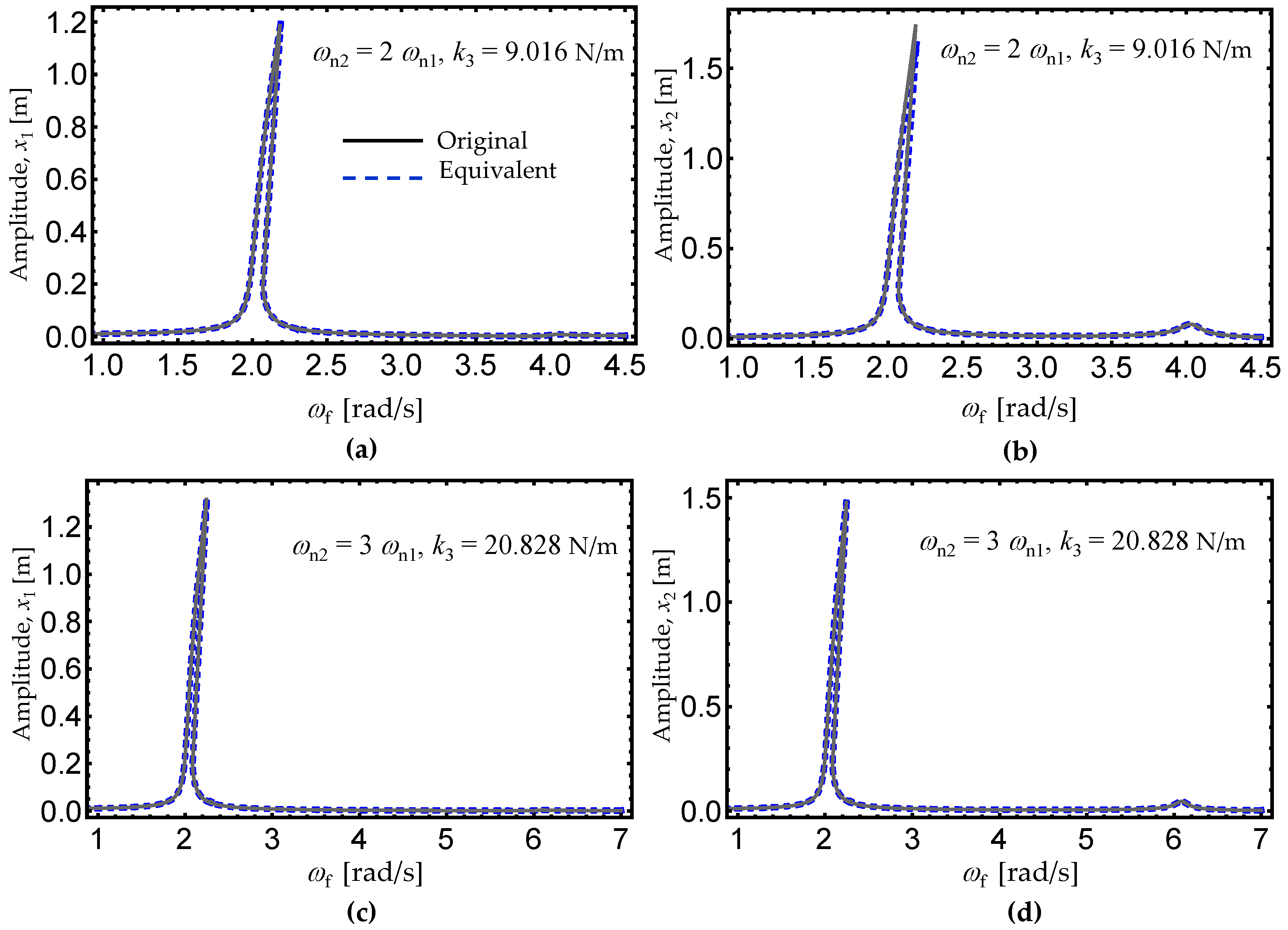
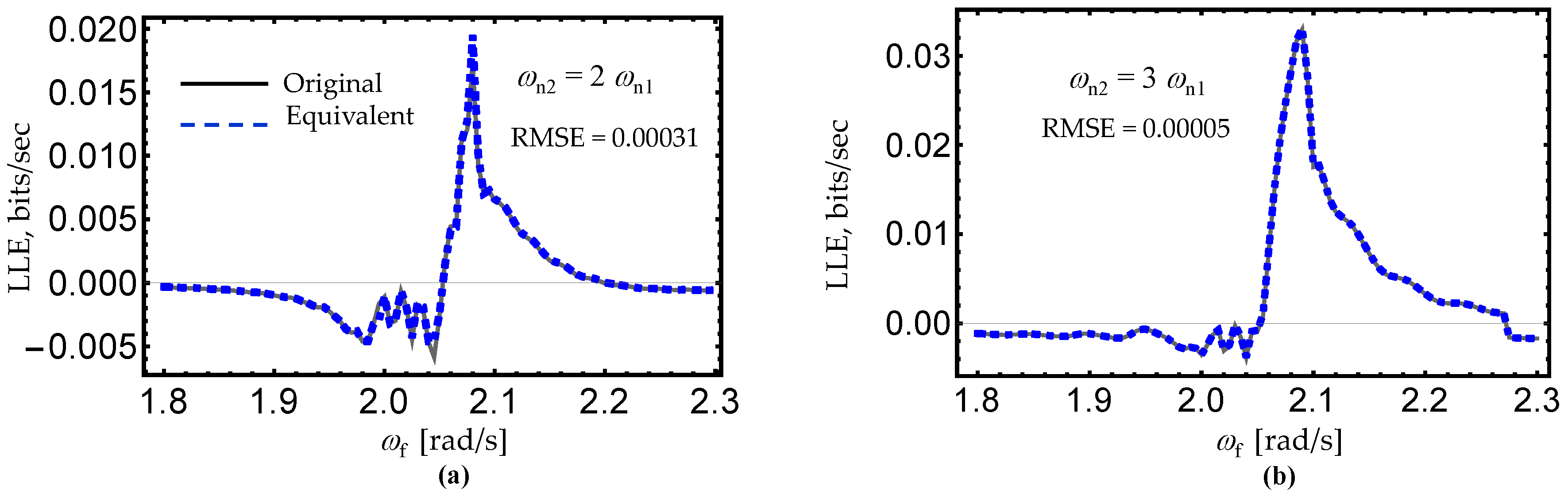
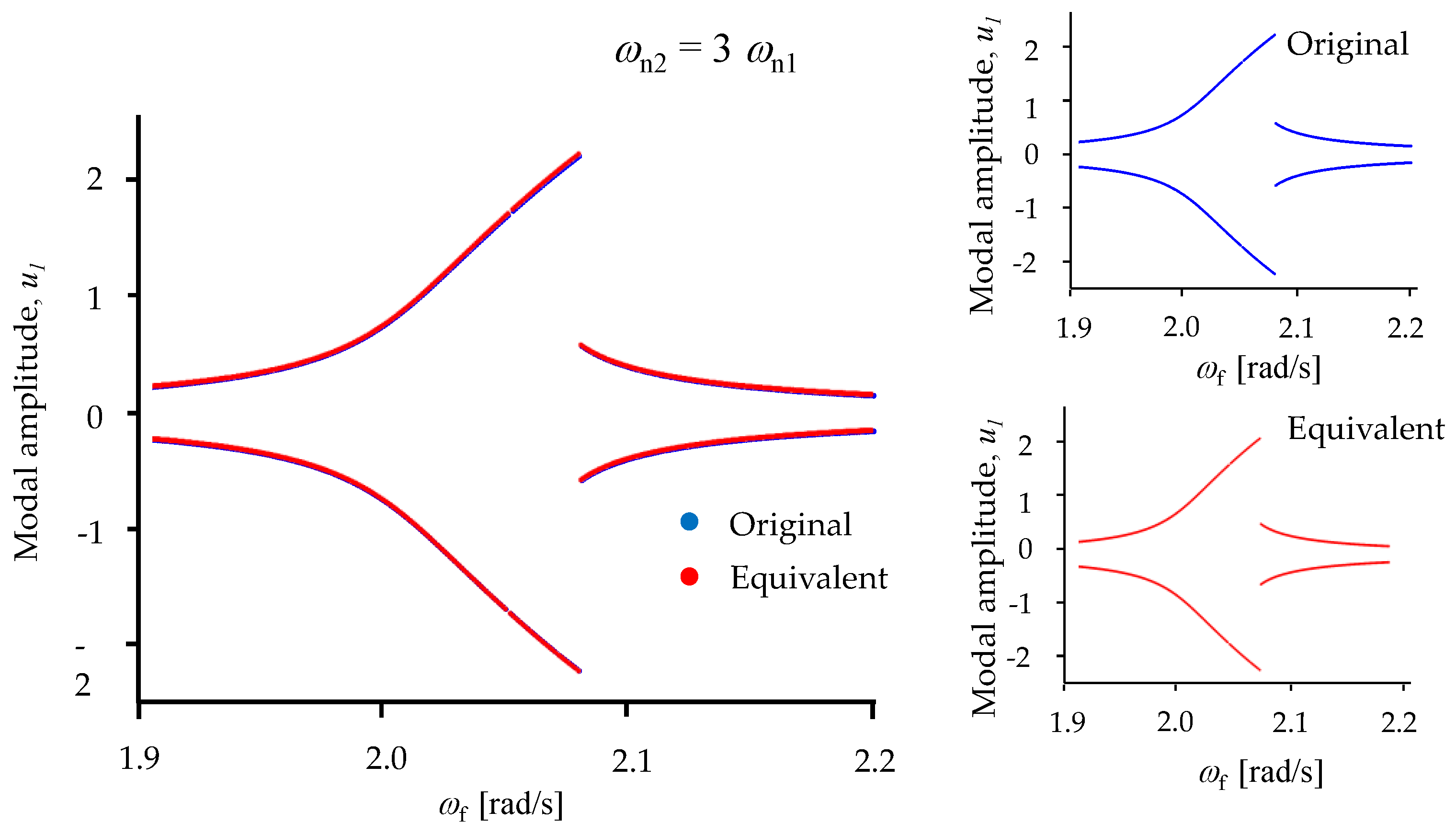
4.3. Example 3: A Nonlinear Absorber System

The following equations of motion,

$$\begin{array}{l}\left[\begin{array}{cc}{m}_1& 0\\ 0& m_2\end{array}\right]\left\{\begin{array}{c}{\ddot{x}}_1\\ {\ddot{x}}_2\end{array}\right\}+\left[\begin{array}{cc}{c}_1+c_2& -c_2\\ -c_2& c_2\end{array}\right]\left\{\begin{array}{c}{\dot{x}}_1\\ {\dot{x}}_2\end{array}\right\}+\left[\begin{array}{cc}{k}_1+k_3& -k_3\\ -k_3& k_3\end{array}\right]\left\{\begin{array}{c}{x}_1\\ x_2\end{array}\right\}+\left\{\begin{array}{c}{k}_2{x}_1^3+k_4{\left(x_1-x_2\right)}^3\\ -k_4{\left(x_1-x_2\right)}^3\end{array}\right\}\\ =\left\{\begin{array}{c}{f}_0\cos {\omega }_{f}t\\ 0\end{array}\right\},\end{array}$$

(43)

describe the dynamics of a nonlinear absorber attached to a single degree-of-freedom nonlinear oscillator [50]. Here, $x_1$, $m_1$, $k_1$, $k_2$ and $c_1$ represent the displacement, mass, linear and nonlinear stiffnesses, and damping coefficient of the primary system, respectively, while $x_2$, $m_2$, $k_3$, $k_4$ and $c_2$ are system parameters related to the nonlinear secondary absorber system, and $f_0$ and ${\omega }_f$ are the external excitation force and driving frequency, respectively.

It is easy to show that system (43) has the normal canonical modal representation form (4) with

$${\phi }_1=r_1^4\left[k_2+k_4\left(f_1+1\right){\left(f_1-3\right)}^3\right],{\phi }_2=3r_1^3{r}_2\left[k_2+k_4{\left(f_1-1\right)}^2\left(f_1+1\right)\left(f_2-1\right)\right],$$

(44)

$${\phi }_3=3r_1^2{r}_2^2\left[k_2+k_4\left(f_1^2-1\right){\left(f_2-1\right)}^2\right],{\phi }_4=r_1^3{r}_2\left[k_2+k_4\left(f_1+1\right){\left(f_1-3\right)}^3\right],$$

(45)

$${\phi }_5=r_1^3{r}_2\left[k_2+k_4{\left(f_1-1\right)}^3\left(f_2+1\right)\right],{\phi }_6=3r_1^2{r}_2^2\left[k_2+k_4{\left(f_1-1\right)}^2{\left(f_2^2-1\right)}^2\right],$$

(46)

$${\phi }_7=3r_1{r}_2^3\left[k_2+k_4\left(f_1-1\right){\left(f_2-1\right)}^2\left(f_2+1\right)\right],{\phi }_8=r_2^4\left[k_2+k_4{\left(f_2-1\right)}^3\left(f_2+1\right)\right],$$

(47)

$${\nu }_1=r_1^2\left[c_1+c_2{\left(f_1-1\right)}^2\right],{\nu }_2=r_1{r}_2\left[c_1+c_2\left(f_1-1\right)\left(f_2-1\right)\right],{\nu }_3=r_2^2\left[c_1+c_2{\left(f_1-1\right)}^2\right],$$

(48)

$${\omega }_{n1}^2=1/\left(2m_1{m}_2\right)\left\{k_1{m}_2+k_3\left(m_1+m_2\right)-\sqrt{{\left[k_1{m}_2+k_3\left(m_1+m_2\right)\right]}^2-4k_1{k}_3{m}_1{m}_2}\right\}$$

(49)

$${\omega }_{n2}^2=1/\left(2m_1{m}_2\right)\left\{k_1{m}_2+k_3\left(m_1+m_2\right)+\sqrt{{\left[k_1{m}_2+k_3\left(m_1+m_2\right)\right]}^2-4k_1{k}_3{m}_1{m}_2}\right\}$$

(50)

$$f_1=\left(k_1+k_3-{\omega }_{n1}^2{m}_1\right)/k_3,f_2=\left(k_1+k_3-{\omega }_{n2}^2{m}_1\right)/k_3,r_1^2=1/\left(m_1+f_1^2{m}_2\right)$$

(51)

$$r_2^2=\frac{1}{\left(m_1+f_2^2{m}_2\right)},P_1\left(t\right)=f_0{r}_1\cos {\omega }_{f}t,P_1\left(t\right)=f_0{r}_2\cos {\omega }_{f}t.$$

(52)

To obtain the frequency-amplitude response curves of the nonlinear absorber system, the parameter values of $m_1=10$ kg, $m_2=0.6$ kg, $c_1=0.1$ Ns/m, $c_2=0.08$ Ns/m, $k_1=44$ N/m, $k_2=8$ N/m³, $k_3=2$ N/m, $k_4=-0.15$ N/m³, and $f_0=0.37$ N were considered, which are similar to those used in [50]. Figure 8 illustrates the frequency-amplitude response curves obtained from the numerical integrations of Equations (29) and (43), in which the equivalent damping coefficients, ${\mu }_1$ and ${\mu }_2$, are bigger than zero. Figure 8 shows that the decoupled solutions describe the dynamic behavior of the original equations of motion well. The LLE numerically-calculated curves are illustrated in Figure 9. As before, these computed LLE curves agree well along the driving frequency range, since the estimated RMSE value is lower than 0.0017.

Next, the following system parameter values are used to plot the frequency-amplitude curves shown in Figure 10: $m_1=10$ kg, $m_2=0.8$ kg, $c_1=0.1$ Ns/m, $c_2=0.08$ Ns/m, $k_1=44$ N/m, $k_3=2$ N/m, $k_4=-0.65$ N/m³, $f_0=0.37$ N, and $k_2=0$ and 8 N/m³. As can be seen from Figure 10, the frequency-amplitude curves obtained using the corresponding decoupled expressions follow closely, in spite of having an absorber device that can have linear or nonlinear stiffness effects; these curves are obtained by numerically integrating the original expressions (43). In this case, the corresponding LLE-computed curves for the original and equivalent equations in the sense of Lyapunov are shown in Figure 11.

To further assess the accuracy of the proposed approach, the values of $k_3=9.016$ N/m, and 20.828 N/m with $m_2=0.6$ kg were used to excite internal resonances of the types, ${\omega }_{n2}=2{\omega }_{n1}$ and ${\omega }_{n2}=3{\omega }_{n1}$, which are second-order and third-order internal resonance relationships, respectively. Figure 12 illustrates the frequency-amplitude curves obtained from the numerical integration solutions of Equations (29) and (43).

It is evident that the equivalent equations in the sense of Lyapunov capture both types of internal resonances without any additional assumptions or simplifications in the method. The estimated LLE curves for the original and equivalent equations are shown in Figure 13. From Figure 13, it is very interesting to see the agreement in the computed LLE curves which is also confirmed by the computed RMSE values and by the bifurcation diagrams shown in Figure 14 and Figure 15. As a consequence, one can conclude that the proposed conjecture is true, i.e., the decoupled Duffing Equations (29) are equivalent, in the sense of Lyapunov, to the normal canonical form of the original equations of motion (43) if the system’s nonlinearities are small and the oscillation amplitudes are moderate. In other words, although our proposed approach is straightforward and easy to apply, this uncoupling process could be only justifiable for small deviations in the system’s linear behavior because, for large amplitudes, coupling and nonlinear terms are important. However, in spite of these drawbacks, the proposed decoupling technique can capture internal resonances, something that is cumbersome when applying other techniques [38,51]. Of course, further investigation into the applicability of this approach to the prediction of internal resonances in other dynamic systems and its potential advantages or disadvantages are beyond the scope of this paper, and these issues will be addressed in a forthcoming article.

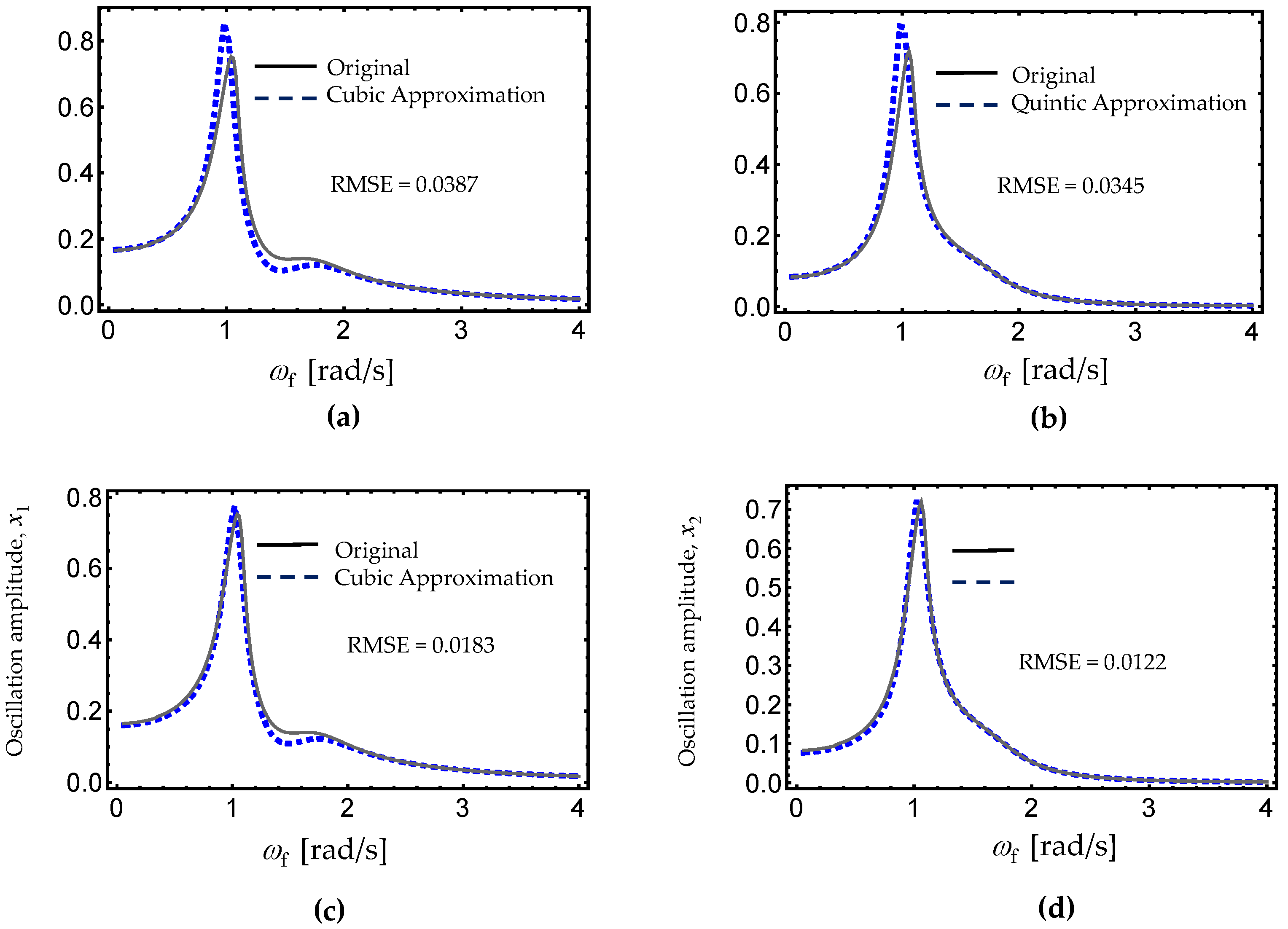
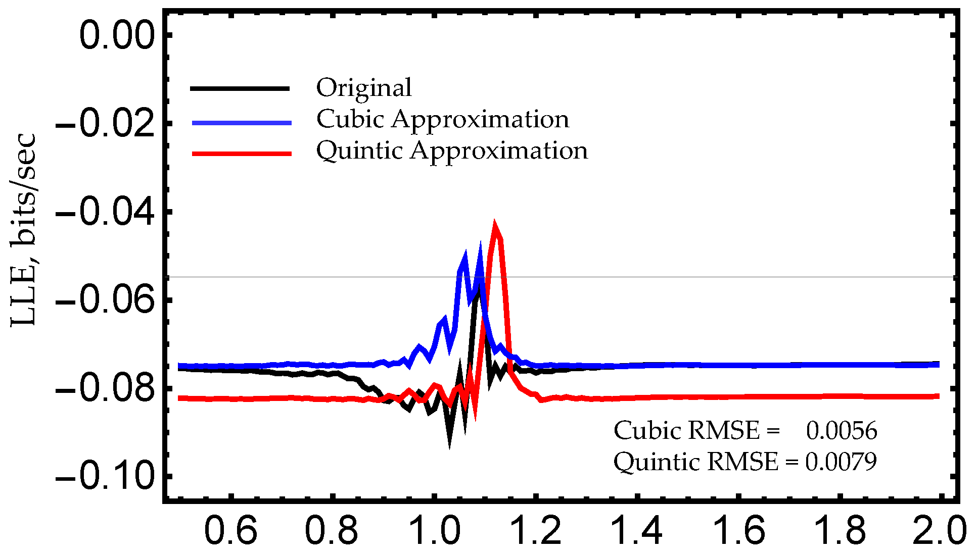
5. Fifth-Order Power Series Expansion

It is important to bear in mind that the predictions obtained in the above examples consider a truncated power series to replace the nonlinear restoring forces, $f_i=\left(x_1,x_2\right)$, by uncoupled cubic polynomial expressions, which, if inaccurate, would cause the conjecture to be false. In an attempt to avoid this situation, the modal system (4) was next replaced by a truncated fifth-order power series expansion that contained nonlinear damping terms [13,38,51,52,53]. As usual, driving forces were assumed to remain constant during the transformation approach. The uncoupled dynamic equations of motion are now written as

$$\begin{array}{r}{\ddot{u}}_1+{\omega }_{n1}^2{u}_1+{\nu }_1{\dot{u}}_1+{\nu }_2{\dot{u}}_2+{\phi }_1{u}_1^3+{\phi }_2{u}_1^2{u}_2+{\phi }_3{u}_1{u}_2^2+{\phi }_4{u}_2^3\\ \equiv {\ddot{u}}_1+a_1{u}_1+a_2{u}_1^3+a_2{u}_1^5+2{\mu }_1{\dot{u}}_1+{\mu }_2{u}_1{\dot{u}}_1^2+{\mu }_3{u}_1^2{\dot{u}}_1+\cdots =P_1\left(t\right),\end{array}$$

(53)

$$\begin{array}{r}{\ddot{u}}_2+{\omega }_{n2}^2{u}_2+{\nu }_2{\dot{u}}_1+{\nu }_3{\dot{u}}_2+{\phi }_5{u}_1^3+{\phi }_6{u}_1^2{u}_2+{\phi }_7{u}_1{u}_2^2+{\phi }_8{u}_2^3\\ \equiv {\ddot{u}}_2+b_1{u}_2+b_2{u}_2^3+b_3{u}_2^5+2{\mu }_4{\dot{u}}_2+{\mu }_5{u}_2{\dot{u}}_2^2+{\mu }_6{u}_2^2{\dot{u}}_2+\cdots =P_2\left(t\right).\end{array}$$

(54)

The Expressions (53) and (54) provide equivalent decoupled representation forms, in the sense of Lyapunov, of the original equations of motion whose accuracy depends on the unknown coefficients: $a_i$, $b_i$, and ${\mu }_i$. By following the procedure described in Section 3, the coefficients, $a_i$, $b_i$, and ${\mu }_i$, were found to be

$$a_1={\omega }_{n1}^2+\frac{1206645{\phi }_1{\eta }_1{\eta }_2}{10446976{\eta }_1}+\frac{394725}{614528{\eta }_1}\left({\phi }_4{\eta }_2^3+2{\nu }_2{V}_2\right)+\frac{{\phi }_3{\eta }_2^2}{3},$$

(55)

$$a_2={\phi }_1+\frac{105\left[57921{\phi }_1{\eta }_1^2{\eta }_2-109055\left({\phi }_4{\eta }_2^3+2{\nu }_2{V}_2\right)\right]}{10446976{\eta }_1^3},$$

(56)

$$a_3=\frac{231\left[-9199{\phi }_1{\eta }_1^2{\eta }_2+31659\left({\phi }_4{\eta }_2^3+2{\nu }_2{V}_2\right)\right]}{10446976{\eta }_1^5},$$

(57)

$${\mu }_1=\frac{17\left(4875{\phi }_4{\eta }_2^3+19204{\nu }_1{V}_1+9750{\nu }_2{V}_2\right)-2727{\phi }_2{\eta }_1^2{\eta }_2}{652936V_1},$$

(58)

$${\mu }_2=\frac{135\left[1013{\phi }_2{\eta }_1^2{\eta }_2-35275\left({\phi }_4{\eta }_2^3+2{\nu }_2{V}_2\right)\right]}{10446976{\eta }_1{V}_1^2},$$

(59)

$${\mu }_3=\frac{3\left[-52{\phi }_2{\eta }_1^2{\eta }_2+3825\left({\phi }_4{\eta }_2^3+2{\nu }_2{V}_2\right)\right]}{81617{\eta }_1^2{V}_1},$$

(60)

$$b_1={\omega }_{n2}^2+\frac{15\left(447355{\phi }_5{\eta }_{11}^3+804432{\phi }_7{\eta }_{11}{\eta }_{22}^2+894710{\nu }_2{V}_{11}\right)}{10446976{\eta }_{22}}+\frac{{\phi }_6{\eta }_{11}^2}{3},$$

(61)

$$b_2=\frac{34\left(307264{\phi }_8{\eta }_{22}^3-673575{\nu }_2{V}_{11}\right)+6081705{\phi }_7{\eta }_{11}{\eta }_{22}^3-11450775{\phi }_5{\eta }_{11}^3}{10446976{\eta }_{11}^3},$$

(62)

$$b_3=\frac{231\left(31659{\phi }_5{\eta }_{11}^3-9199{\phi }_7{\eta }_{11}{\eta }_{22}^2+63138{\nu }_2{V}_{11}\right)}{10446976{\eta }_{22}^5},$$

(63)

$${\mu }_4=\frac{{\nu }_3}{2}+\frac{3\left(27625{\phi }_5{\eta }_{11}^3-909{\phi }_7{\eta }_{11}{\eta }_{22}^2+55250{\nu }_2{V}_{11}\right)}{652936V_{22}},$$

(64)

$${\mu }_5=-\frac{135\left(35275{\phi }_5{\eta }_{11}^3-1013{\phi }_7{\eta }_{11}{\eta }_{22}^2+70550{\nu }_2{V}_{11}\right)}{10446976{\eta }_{22}{V}_{22}^2},$$

(65)

$${\mu }_6=\frac{3\left(3825{\phi }_5{\eta }_{11}^3-52{\phi }_7{\eta }_{11}{\eta }_{22}^2+7650{\nu }_2{V}_{11}\right)}{10446976{\eta }_{22}{V}_{22}^2}.$$

(66)

The values of ${\eta }_i$, ${\eta }_{ii}$, $V_i$, and $V_{ii}$ were obtained by minimizing the following expressions:

$$\begin{array}{c}{U}_1=\min \underset{0}{\overset{V_2}{{\displaystyle \int }}}\underset{0}{\overset{V_1}{{\displaystyle \int }}}\underset{0}{\overset{{\eta }_2}{{\displaystyle \int }}}\underset{0}{\overset{{\eta }_1}{{\displaystyle \int }}}({\omega }_{n1}^2{u}_1+{\nu }_1{\dot{u}}_1+{\nu }_2{\dot{u}}_2+{\phi }_1{u}_1^3+{\phi }_2{u}_1^2{u}_2+{\phi }_3{u}_1{u}_2^2+{\phi }_4{u}_2^3-a_1{u}_1-a_2{u}_1^3\\ -a_3{u}_1^5-2{\mu }_1{\dot{u}}_1-{\mu }_2{u}_1{\dot{u}}_1^2-{\mu }_3{u}_1^2{\dot{u}}_1){}^2 d{u}_1 d{u}_2 d{\dot{u}}_1 d{\dot{u}}_2,\end{array}$$

(67)

$$\begin{array}{c}{U}_2=\min \underset{0}{\overset{V_{11}}{{\displaystyle \int }}}\underset{0}{\overset{V_{22}}{{\displaystyle \int }}}\underset{0}{\overset{{\eta }_{11}}{{\displaystyle \int }}}\underset{0}{\overset{{\eta }_{22}}{{\displaystyle \int }}}({\omega }_{n2}^2{u}_2+2{\nu }_2{\dot{u}}_1+{\nu }_3{\dot{u}}_2+{\phi }_5{u}_1^3+{\phi }_6{u}_1^2{u}_2+{\phi }_7{u}_1{u}_2^2+{\phi }_8{u}_2^3-b_1{u}_2-b_2{u}_2^3\\ -b_3{u}_2^5-2{\mu }_4{\dot{u}}_2-{\mu }_5{u}_2{\dot{u}}_2^2-{\mu }_6{u}_2^2{\dot{u}}_2){}^{2}d{u}_2 d{u}_1 d{\dot{u}}_2 d{\dot{u}}_1.\end{array}$$

(68)

For comparison purposes, only the dynamic system examined in Example 1 was considered, since the oscillators studied in Examples 2 and 3 had small errors when the equivalent expressions in the sense of Lyapunov were compared to the original equations of motion. First, we focused on studying the unforced dynamic system (30) and plotted the amplitude-time curves by using the equivalent cubic, and quintic expressions: (29), (53) and (54). The parameter values selected were $m=1$, $k=1$, $c=0.3$, $\epsilon =0.5$, with $\left(x_1, x_2, {\dot{x}}_1, {\dot{x}}_2\right)=\left(0, 0, 2, 0\right)$. Projection of the initial condition onto the linear transformation (3), yielded $\left(u_{10}, u_{20}, {\dot{u}}_{10}, {\dot{u}}_{20}\right)=\left(1.9118,-0.9165,0,0\right).$ Figure 16 shows the time-amplitude curves for the two modes of the system. Notice that as a consequence of the fifth-order and nonlinear decay terms of the quintic approach, the equivalent representation forms (53) and (54) provide an improvement in the RMSE values. Next, the driving force magnitude of $f_1=0.25$ was considered and then, the frequency-amplitude response, as well as the LLE curves were plotted. As can be seen in Figure 17, the quintic equivalent representation form in the sense of Lyapunov provided a better approximation to the exact numerical values. An improvement was achieved in the frequency-amplitude response curves obtained from the quintic approach since the estimated curves match the numerical results well; however, one can notice from Figure 18, that when the quintic approach is used to compute the LLE values, the RMSE value is slightly higher than that computed by using the cubic model, which is mainly due to the numerical procedure used to compute these values rather than to the decoupling proposed approach.

Based on these results, one can conclude that the improvement of the numerical prediction obtained from the equivalent representation forms will depend on the physical system, its nonlinearities, and its initial condition values.

6. Conclusions

A transformation approach has been proposed to find the equivalent representation form in the sense of Lyapunov of forced, damped, nonlinear, two degree-of-freedom dynamic systems. This proposed approach of finding equivalent expressions has the main advantage of providing simple algebraic relations whose coefficient values are determined by minimizing the error of replacing the original restoring forces by equivalent ones. By studying the dynamic responses of three nonlinear dynamic systems, the validity of the proposed conjecture has been numerically examined by comparing the LCEs of the original equations with those obtained from their equivalent uncoupled expressions. From the numerical predictions obtained, it is concluded that the LCEs and the LLE of the equivalent expression are similar to those obtained from the original equations of motion. In fact, numerical results have shown that the proposed procedure predicts the quantitative behavior of the nonlinear systems examined here well; however, there are some discrepancies which could be removed if additional terms in the power series expansion of the dynamical system’s restoring forces are considered. Furthermore, when the system’s restoring forces were replaced by a fifth-order truncated power series expansion in which decay rate terms were considered, numerical predictions computed from the nonlinear dynamic system of Example 1, indicated that the RMSE values were lower than those of the cubic truncated power series expansion, since, in this quintic approach, decay rate terms were considered. In this case, both the qualitative and the quantitative dynamic system behaviors in physical coordinates were predicted well in spite of having uncoupled modal equivalent oscillators, as shown in Figure 16 and Figure 17.

Finally, and contrary to other proposed approaches, the one introduced here is capable of describing the dynamic behavior of nonlinear systems when internal resonance exists between the two modes, and thus, it is possible to uncouple, in modal coordinates, the resonant modes, as illustrated in Figure 12. Therefore, it can be concluded, in accordance with the numerical evidence of the dynamic systems examined here, that it is possible to have two decoupled Duffing-type equivalent representation forms of the original equations of motion in the sense of Lyapunov that can predict the dynamics of the original system, and accuracy can be improved if additional terms in the truncated power series are considered, not only to describe elastic forces, but also to take into account decay rate effects.

Of course, the system’s restoring forces could be replaced by other forms rather than Duffing-type equivalent representation expressions.

However, the applicability of the proposed approach to other nonlinear dynamic systems by using truncated power series expansions or alternative forms to replace the system restoring forces could be considered only for small deviations of the system’s linear behavior, because for large amplitudes, coupling and nonlinear terms are important.

References

1. Minorsky, N. Introduction to non-linear mechanics, Part II, Analytical Methods of Non-Linear Mechanics. The David W. Taylor Model Basin U. S. N. Report #546. MIT Libraries: Cambridge MA USA, September 1945. [Google Scholar]
2. Caughey, T.K. Equivalent linearisation techniques. J. Acoust. Soc. Am. 1963, 35, 1706–1711. [Google Scholar] [CrossRef]
3. Iwan, W.D. On defining equivalent systems for certain ordinary non-linear differential equations. Int. J. Non-Linear Mech. 1969, 4, 325–334. [Google Scholar] [CrossRef]
4. Iwan, W.D. A generalization of the concept of equivalent linearization. Int. J. Non-Linear Mech. 1973, 4, 279–287. [Google Scholar] [CrossRef]
5. Shina, S.C.; Srinivasan, P. A weighted mean square method of linearization in non-linear oscillators. J. Sound Vib. 1971, 16, 139–148. [Google Scholar]
6. Agrwal, V.P.; Denman, H.H. Weighted linearization technique for period approximation in large amplitude non-linear oscillations. J. Sound Vib. 1985, 99, 463–473. [Google Scholar] [CrossRef]
7. Yuste, S.B.; Sánchez, A.M. A weighted mean-square method of cubication for non-linear oscillators. J. Sound Vib. 1989, 134, 423–433. [Google Scholar] [CrossRef]
8. Yuste, S.B. Cubication of non-linear oscillators using the principle of harmonic balance. Int. J. Non-Linear Mech. 1992, 27, 347–356. [Google Scholar] [CrossRef]
9. Cai, J.; Wu, X.; Li, Y.P. An equivalent nonlinearization method for strongly nonlinear oscillations. Mech. Res. Commun. 2005, 32, 553–560. [Google Scholar] [CrossRef]
10. Farzaneh, Y.; Tootoonchi, A.A. Global Error Minimization method for solving strongly nonlinear oscillator differential equations. Comput. Math. Appl. 2010, 59, 2887–2895. [Google Scholar] [CrossRef]
11. Elías-Zúñiga, A.; Olvera Trejo, D.; Ferrer Real, I.; Martínez-Romero, O. A Transformation Method for Solving Conservative Nonlinear Two Degree-of-Freedom Systems. Math. Probl. Eng. 2014, 2014, 237234. [Google Scholar] [CrossRef]
12. Bhattacharyya, R.; Jain, P.; Nair, A. Normal model localization for a two degrees-of-freedom system with quadratic and cubic non-linearities. J. Sound Vib. 2002, 249, 909–919. [Google Scholar] [CrossRef]
13. Touzé, C.; Thomas, O.; Chaigne, A. Hardening/softening behaviour in nonlinear oscillations of structural systems using non-linear normal modes. J. Sound Vib. 2004, 273, 77–101. [Google Scholar] [CrossRef]
14. Alexander, N.A.; Schilder, F. Exploring the performance of a nonlinear tuned mass damper. J. Sound Vib. 2009, 319, 445–462. [Google Scholar] [CrossRef]
15. Pirbodaghi, T.; Hoseini, S. Nonlinear Free Vibration of a Symmetrically Conservative Two-Mass System With Cubic Nonlinearity. J. Comput. Non-Linear Dyn. 2010, 5, 011006-1–011006-6. [Google Scholar] [CrossRef]
16. Trueba, J.L.; Rams, J.; Sanjuán, M.A.F. Analytical estimates of the effect of nonlinear damping in some nonlinear oscillators. Int. J. Bifurc. Chaos 2000, 10, 2257–2267. [Google Scholar] [CrossRef]
17. Elías-Zúñiga, A.; Martínez-Romero, O. Accurate Solutions of Conservative Nonlinear Oscillators by the Enhanced Cubication Method. Math. Probl. Eng. 2013, 2013, 842423. [Google Scholar] [CrossRef]
18. Rand, R.H. Nonlinear Normal Modes in Two-Degree-of-Freedom Systems. J. Appl. Mech. 1971, 38, 561. [Google Scholar] [CrossRef]
19. Rand, R.H. The Geometrical Stability of Non-Linear Normal Modes in Two Degree of Freedom Systems. Int. J. Non-Linear Mech. 1973, 8, 161–168. [Google Scholar] [CrossRef]
20. Shaw, S.W.; Pierre, C. Normal Modes for Non-Linear Vibratory Systems. J. Sound Vib. 1993, 164, 85–124. [Google Scholar] [CrossRef]
21. Jiang, D.; Pierre, C.; Shaw, S.W. Nonlinear normal modes for vibratory systems under harmonic excitation. J. Sound Vib. 2005, 288, 791–812. [Google Scholar] [CrossRef]
22. Nayfeh, A.H.; Mook, D.T. Non-Linear Oscillations; John-Willey: New-York, NY, USA, 1979. [Google Scholar]
23. Nayfeh, A.H.; Sanchez, N.E. Bifurcations in a forced softening Duffing oscillator. Int. J. Non-Linear Mech. 1989, 24, 483–497. [Google Scholar] [CrossRef]
24. Okabea, T.; Kondou, T. Improvement to the averaging method using the Jacobian elliptic function. J. Sound Vib. 2009, 320, 339–364. [Google Scholar] [CrossRef]
25. Koshlyakov, V.N.; Makarov, V.L. Mechanical systems, equivalent in Lyapunov’s sense to systems not containing non-conservative positional forces. J. Appl. Math. Mech. 2007, 71, 10–19. [Google Scholar] [CrossRef]
26. Zalygina, V.I. Lyapunov Equivalence of Systems with Unbounded Coefficients. J. Math. Sci. 2015, 210, 210–216. [Google Scholar] [CrossRef]
27. Peeters, M.; Viguié, R.; Sérandour, G.; Kerschen, G.; Golinval, J.-C. Nonlinear normal modes, part II: Toward a practical computation using numerical continuation techniques. Mech. Syst. Signal Process. 2009, 23, 195–216. [Google Scholar] [CrossRef]
28. Dick, A.J.; Balachandran, B.; Mote, C.D. Intrinsic localized modes in microresonator arrays and their relationship to nonlinear vibration modes. Nonlinear Dyn. 2008, 54, 13–29. [Google Scholar] [CrossRef]
29. Bellet, R.; Cochelin, B.; Herzog, P.; Mattei, P.-O. Experimental study of targeted energy transfer from an acoustic system to a nonlinear membrane absorber. J. Sound Vib. 2010, 329, 2768–2791. [Google Scholar] [CrossRef]
30. Yan, Y.; Wang, W.; Zhang, L. Applied multiscale method to analysis of nonlinear vibration for double-walled carbon nanotubes. Appl. Math. Model. 2011, 35, 2279–2289. [Google Scholar] [CrossRef]
31. Kerschen, G.; Peeters, M.; Golinval, J.-C.; Stephan, C. Nonlinear modal analysis of a full-scale aircraft. J. Aircr. 2013, 50, 1409–1419. [Google Scholar] [CrossRef]
32. Renson, L.; Noël, J.P.; Kerschen, G. Complex dynamics of a nonlinear aerospace structure: Numerical continuation and normal modes. Nonlinear Dyn. 2015, 79, 1293–1309. [Google Scholar] [CrossRef]
33. Kuether, R.J.; Allen, M.S.; Hollkamp, J.J. Modal substructuring of geometrically nonlinear finite-element models. AIAA J. 2015, 54, 691–702. [Google Scholar] [CrossRef]
34. Kuether, R.J.; Deaner, B.J.; Hollkamp, J.J.; Allen, M.S. Evaluation of geometrically nonlinear reduced-order models with nonlinear normal modes. AIAA J. 2015, 53, 3273–3285. [Google Scholar] [CrossRef]
35. Lacarbonara, W.; Carboni, B.; Quaranta, G. Nonlinear normal modes for damage detection. Meccanica 2016, 51, 1–17. [Google Scholar] [CrossRef]
36. Meirovitch, L. Elements of Vibration Analysis; McGraw-Hill Book Company: New York, NY, USA, 1986. [Google Scholar]
37. Barabanov, E.A. Maximal Linear Transformation Groups Preserving the Asymptotic Properties of Linear Differential Systems: II. Differ. Equ. 2012, 48, 1545–1562. [Google Scholar] [CrossRef]
38. Touzé, C.; Amabili, M. Nonlinear normal modes for damped geometrically nonlinear systems: Application to reduced-order modelling of harmonically forced structures. J. Sound Vib. 2006, 298, 958–981. [Google Scholar] [CrossRef]
39. Elías-Zúñiga, A. A General Solution of the Duffing Equation. Nonlinear Dyn. 2006, 45, 227–235. [Google Scholar] [CrossRef]
40. Wolf, A.; Swift, J.B.; Swinney, H.L.; Vastano, J.A. Determining Lyapunov Exponents from a time series. Phys. D Nonlinear Phenom. 1985, 16, 285–317. [Google Scholar] [CrossRef]
41. Sandri, M. Numerical calculations of Lyapunov exponents. Math. J. 1996, 6, 78–84. [Google Scholar]
42. Kerschen, G.; Peeters, M.; Golinval, J.C.; Vakakis, A.F. Nonlinear normal modes, Part I: A useful frame work for the structural dynamicist. Mech. Syst. Signal Process. 2009, 23, 170–194. [Google Scholar] [CrossRef]
43. Blumberg, H. On Convex Functions. Trans. Am. Math. Soc. 1919, 20, 40–44. [Google Scholar] [CrossRef]
44. Boyd, S.; Vandenberghe, L. Convex Optimization; Cambridge University Press: Cambridge, UK, 2009; pp. 67–74. [Google Scholar]
45. Soriano, J.M. Global Minimum Point of a Convex Function. Appl. Math. Comput. 1993, 55, 213–218. [Google Scholar] [CrossRef]
46. Barbu, V.; Precupanu, T. Convexity and Optimization in Banach Spaces; Springer Monographs in Mathematics; Springer Science & Business Media: Berlin, Germany; Springer: New York, NY, USA, 2012. [Google Scholar] [CrossRef]
47. Hsu, C.S. On the application of elliptic functions in nonlinear forced oscillations. Q. Appl. Math. 1960, 17, 393–407. [Google Scholar] [CrossRef]
48. Chen, S.H.; Cheung, Y.K. A modified Lindstedt-Poincare method for a strongly non-linear two degree-of-freedom-system. J. Sound Vib. 1996, 193, 751–762. [Google Scholar] [CrossRef]
49. Franciosi, C.; Tomasiello, S. The use of Mathematica for the analysis of strongly nonlinear two degree-of-freedom systems by means of the modified Lindstedt-Poincaré method. J. Sound Vib. 1998, 211, 145–156. [Google Scholar] [CrossRef]
50. Ji, J.C. Application of a Weakly Nonlinear Absorber to Suppress the Resonant Vibrations of a Forced Nonlinear Oscillator. J. Vib. Acoust. 2012, 134, 044502. [Google Scholar] [CrossRef]
51. Vakakis, A.F. Nonlinear normal modes (NNMs) and their application in vibration theory: An overview. Mech. Syst. Signal Process. 1997, 11, 3–22. [Google Scholar] [CrossRef]
52. Elías-Zúñiga, A.; Martínez-Romero, O. Investigation of the equivalent representation form of damped strongly nonlinear oscillators by a nonlinear transformation approach. J. Appl. Math. 2013, 2013, 245092. [Google Scholar] [CrossRef]
53. Blanc, F.; Touzé, C.; Mercier, F.F.; Ege, K.; Ben-Dhia, A.S.B. On the numerical computation of nonlinear normal modes for reduced-order modelling of conservative vibratory systems. Mech. Syst. Signal Process. 2013, 36, 520–539. [Google Scholar] [CrossRef]
Figure 1. Modal amplitudes: (a) u1 vs ω1, (b) u2 vs ω2. The backbone curves were computed from Equations (33) to (35). The parameter values used to obtain these plots were m 1 = m 2 = 1 , k = 1 , ε = 0.5 with c = 0 and f 1 = 0 . Here, the black solid lines describe the solutions obtained from Equations (34) and (35), while the blue dashed lines represent the backbone curves computed from Equation (33).
Applsci 08 00649 g001
Figure 2. Modal amplitudes: (a) u1 vs ω1, (b) u2 vs ω2. The backbone curves were computed from Equations (33) to (35). The parameter values used to obtain these plots for different values of k and ε were m 1 = m 2 = 1 , with c = 0 and f 1 = 0 . Here, the black solid lines describe the solutions obtained from Equations (34) and (35), while the colored, dashed lines represent the backbone curves computed from Equation (33).
Applsci 08 00649 g002
Figure 3. Time-amplitude response curves (a) x1 vs t, (b) x2 vs t. These were computed from the numerical integration solutions of Equations (29) and (30). The parameter values used to obtain these plots were m 1 = m 2 = 1 , k = 1 , ε = 0.5 with c = 0.3 , with initial conditions given by ( x 1 ,   x 2 ,   x ˙ 1 ,   x ˙ 2 ) = ( 0 ,   0 ,   2 ,   0 ) . Here, the black lines describe the numerical integration solutions of Equation (30), while the blue, dashed lines represent the numerical solutions obtained from the nonlinear equations of motion (29).
Applsci 08 00649 g003
Figure 4. Frequency-amplitude response curves: (a) x1 vs ωf, (b) x2 vs ωf. These were computed from the numerical integration solutions of Equations (29) and (30). The parameter values used to obtain these plots were m 1 = m 2 = 1 , k = 1 , ε = 0.5 with c = 0.3 and f 1 = 0.25 . Here, the black solid lines describe the numerical integration solutions of Equation (30), while the blue dashed lines represent the numerical solutions obtained from Equation (29).
Applsci 08 00649 g004
Figure 5. Largest Lyapunov Characteristic Exponent (LLE) curves computed from the numerical integration solutions of Equations (29) and (30). The parameter values used to obtain these plots were m 1 = m 2 = 1 , k = 1 and ε = 0.5 with c = 0.3 and f 1 = 0.25 . Here, the black, solid line represents the LLE computed from the numerical integration solutions of Equation (30), while the blue, dashed line describes the LLE obtained from Equation (29).
Applsci 08 00649 g005
Figure 6. Frequency-amplitude response curves: (a) x1 vs ωf, (b) x2 vs ωf. These were computed from the numerical integration solutions of Equations (36) and (42). The parameter values used to obtain these plots were m 1 = 1 kg, m 2 = 1.5 kg, k 1 = 2 N/m, k 2 = 3.5 N/m, k 3 = 5 N/m, c 1 = 0.066 N-s/m, c 2 = 0.099 N-s/m, ε 1 = 1   N /m3, ε 2 = 1 N/m3, Q 1 = 0.2 N. Here, the black, solid lines describe the numerical integration solutions of Equations (36), while the blue, dashed lines represent the numerical solutions obtained from the derived equivalent nonlinear equations of motion (42).
Applsci 08 00649 g006
Figure 7. Amplitude versus time response curves: (a) u1 vs t, (b) u2 vs t, (c) x1 vs t, (d) x2 vs t. Almost periodic solutions can be observed when the modal displacements are transformed back into the original coordinate systems x1 and x2 using the relationships (37). Here the solid line represents the numerical integration solution of Equation (36), while the dashed, colored line describes the approximate solution obtained from Equation (42).
Applsci 08 00649 g007
Figure 8. Frequency-amplitude response curves: (a) x1 vs ωf, (b) x2 vs ωf. These were computed from the numerical integration solutions of Equations (29) and (43). The parameter values used to obtain these plots were m 1 = 10 kg, m 2 = 0.6 kg, c 1 = 0.1 Ns/m, c 2 = 0.08 Ns/m, k 1 = 44 N/m,   k 2 = 8 N/m3, k 3 = 2 N/m, k 4 = 0.15 N/m3, f 0 = 0.37 N. Here, the black, solid lines describe the numerical integration solution of Equation (43), while the blue, dashed lines represent the numerical solutions obtained from the derived equivalent nonlinear equations of motion (29).
Applsci 08 00649 g008
Figure 9. LLE curves computed from the numerical integration solutions of Equations (29) and (43). The parameter values used to obtain these plots were m 1 = 10 kg, m 2 = 0.6 kg, c 1 = 0.1 Ns/m, c 2 = 0.08 Ns/m, k 1 = 44 N/m,   k 2 = 8 N/m3, k 3 = 2 N/m, k 4 = 0.15 N/m3, f 0 = 0.37 N. Here, the black line represents the LLE computed from the numerical integration solutions of Equation (43), while the blue line describes the LLE obtained from Equation (29).
Applsci 08 00649 g009
Figure 10. Frequency-amplitude response curves computed from the numerical integration solutions of Equations (29) and (43). The parameter values used to obtain these plots were m 1 = 10 kg, m 2 = 0.8 kg, c 1 = 0.1 Ns/m, c 2 = 0.08 Ns/m, k 1 = 44 N/m, k 3 = 2 N/m, k 4 = 0.65 N/m3, f 0 = 0.37 N, and (a) x1 vs ωf, and (b) x2 vs ωf with k2 = 0; (c) x1 vs ωf, and (d) x2 vs ωf with k2 = 8 N/m3. Here, the black, solid lines describe the numerical integration solution of Equation (43), while the blue, dashed lines represent the numerical solutions obtained from the derived equivalent nonlinear equations of motion (29).
Applsci 08 00649 g010
Figure 11. LLE curves computed from the numerical integration solutions of Equations (29) and (43). The parameter values used to obtain these plots were m 1 = 10 kg, m 2 = 0.8 kg, c 1 = 0.1 Ns/m, c 2 = 0.08 Ns/m, k 1 = 44 N/m, k 3 = 2 N/m, k 4 = 0.65 N/m3, f 0 = 0.37 N, and (a) k 2 = 0 and (b) k 2 = 8 N/m3. Here, the black line represents the LLE computed from the numerical integration solutions of Equation (43), while the blue line describes the LLE obtained from Equation (29).
Applsci 08 00649 g011
Figure 12. Frequency-amplitude response curves computed from the numerical integration solutions of Equations (29) and (43) when subjected to internal resonances. Internal resonance of the type ω n 2 = 2 ω n 1 , (a) x1 vs ωf, (b) x2 vs ωf with k 3 = 9.016   N / m . Internal resonance of the type, ω n 2 = 3 ω n 1 , (c) x1 vs ωf, (d) x2 vs ωf with k 3 = 20.828 N/m. The parameter values used to obtain these plots were m 1 = 10 kg, m 2 = 0.6 kg, c 1 = 0.1 Ns/m, c 2 = 0.08 Ns/m, k 1 = 44 N/m, k 2 = 8 N/m3, k 4 = 0.65 N/m3, and f 0 = 0.37 N. Here, the black, solid lines describe the numerical integration solution of Equation (43), while the blue, dashed lines describe the numerical solutions obtained from the derived equivalent nonlinear equations of motion (29).
Applsci 08 00649 g012
Figure 13. LLE curves computed from the numerical integration solutions of Equations (29) and (43). The parameter values used to obtain these plots were m 1 = 10 kg, m 2 = 0.6 kg, c 1 = 0.1 Ns/m, c 2 = 0.08 Ns/m, k 1 = 44 N/m, k 2 = 8 N/m3, k 4 = 0.65 N/m3, and f 0 = 0.37 N; (a) LLE vs ωf with k 3 = 9.016 N/m, (b) LLE vs ωf with k 3 = 20.828 N/m. Here, the black, solid line represents the LLE computed from the numerical integration solutions of Equation (43), while the blue, dashed line represents the LLE obtained from Equation (29).
Applsci 08 00649 g013
Figure 14. Bifurcation diagrams computed from the numerical integration solutions of Equations (29) and (43). The parameter values used to obtain these curves were m 1 = 10 kg, m 2 = 0.6 kg, c 1 = 0.1 Ns/m, c 2 = 0.08 Ns/m, k 1 = 44 N/m, k 2 = 8 N/m3, k 3 = 9.016 , k 4 = 0.65 N/m3, and f 0 = 0.37 N, with ω n 2 = 2 ω n 1 . Here, the black line represents the bifurcation diagram computed from the numerical integration solutions of Equation (43), while the red line describes the one obtained from Equation (29).
Applsci 08 00649 g014
Figure 15. Bifurcation diagrams computed from the numerical integration solutions of Equations (29) and (43). The parameter values used to obtain these curves were m 1 = 10 kg, m 2 = 0.6 kg, c 1 = 0.1 Ns/m, c 2 = 0.08 Ns/m, k 1 = 44 N/m, k 2 = 8 N/m3, k 3 = 20.828 N/m, k 4 = 0.65 N/m3, and f 0 = 0.37 N, with ω n 2 = 3 ω n 1 . Here, the black line represents the bifurcation diagram computed from the numerical integration solutions of Equation (43), while the red line describes the one obtained from Equation (29).
Applsci 08 00649 g015
Figure 16. Time-amplitude response curves computed from the numerical integration solutions of Equations (53) and (54). Cubic approximation: (a) x1 vs t, (b) x2 vs t. Quintic approximation: (c) x1 vs t, (d) x2 vs t. The parameter values used to obtain these plots were m 1 = m 2 = 1 , k = 1 , ε = 0.5 with c = 0.3 , with initial conditions given by ( x 1 ,   x 2 ,   x ˙ 1 ,   x ˙ 2 ) = ( 0 ,   0 ,   2 ,   0 ) , a 1 = 1.055 , a 2 = 0.1375 , a 3 = 0.0109 , b 1 = 2.9995 , b 2 = 0.1228 , b 3 = 0.0008 , μ 1 = 0.0807 , μ 2 = 0.0206 , μ 3 = 0.0066 , μ 4 = 0.375 , μ 5 = 0 , μ 6 = 0 , with fitting parameter values of η 1 = 1 , η 2 = 0.3 , V 1 = 1 , V 2 = 0.15 , η 11 = 0.01 , η 22 = 1 , V 11 = 0 , V 22 = 1 , and weighted mean square error values of U1 = −2.16 × 10⁻⁵, U2 = 0. Here, the black, solid lines describe the numerical integration solutions of Equation (30), while the blue, dashed lines represent the numerical solutions obtained from the nonlinear equations of motion, (53) and (54).
Applsci 08 00649 g016
Figure 17. Frequency-amplitude response curves computed from the numerical integration solutions of Equations (53) and (54). Cubic approximation: (a) x1 vs ωf, (b) x2 vs ωf. Quintic approximation: (c) x1 vs ωf, (d) x2 vs ωf. The values used to obtain these plots were m 1 = m 2 = 1 , k = 1 , ε = 0.5 with c = 0.3 and f 1 = 0.25 , with fitting parameter values for the quintic approximation of η 1 = 1 , η 2 = 0.3 , V 1 = 1 , V 2 = 0.15 , η 11 = 0.01 , η 22 = 1 , V 11 = 0 , V 22 = 1 , and weighted mean square error values of U 1 = 2.16 × 10 5 , U 2 = 0 . Here, the black, solid lines describe the numerical integration solutions of Equation (30), while the blue, dashed lines are the numerical solutions obtained from the equivalent cubic and quintic expressions, (29), (53) and (54), respectively.
Applsci 08 00649 g017
Figure 18. LLE curves computed from the numerical integration solutions of Equations (29), (30), (53) and (54). The parameter values used to obtain these plots were m 1 = m 2 = 1 , k = 1 , ε = 0.5 with c = 0.3 and f 1 = 0.25 , with fitting parameter values for the quintic approximation of η 1 = 1 , η 2 = 0.3 , V 1 = 1 , V 2 = 0.15 , η 11 = 0.01 , η 22 = 1 , V 11 = 0 , V 22 = 1 , and weighted mean square error values of U 1 = 2.16 × 10 5 , U 2 = 0 . Here, the black line represents the LLE computed from the numerical integration solutions of Equation (30), while the blue and red lines describe the LLE obtained from Equations (29), (53) and (54), respectively.
Applsci 08 00649 g018