Forecasting of Power Grid Investment in China Based on Support Vector Machine Optimized by Differential Evolution Algorithm and Grey Wolf Optimization Algorithm

Abstract

1. Introduction
- (1)
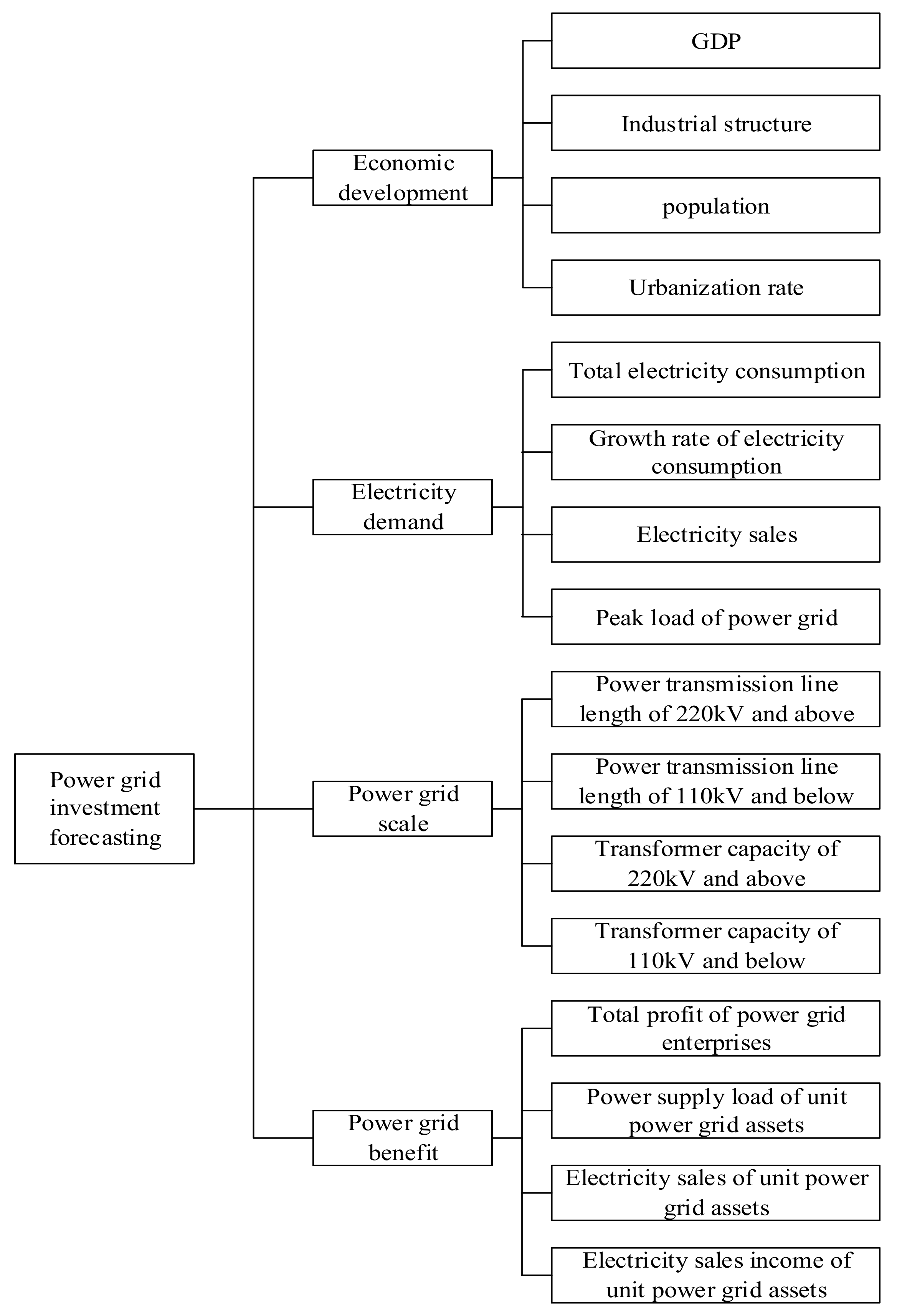
- Power grid investment forecasting in China is affected by many factors. In order to realize the accurate forecasting of China’s power grid investment, relevant factors of power grid investment forecasting are preliminarily selected based on studying a large number of literatures in this article. Through the Delphi method, multiple rounds of anonymous consultations and feedbacks are carried out on experts’ opinions, and the influencing factors system for China’s power grid investment forecasting is finally determined. From the four dimensions of economic development, electricity demand, power grid scale, and power grid benefit, the influencing factors system for power grid investment forecasting is constructed. Then, the method of grey relational analysis is used for screening the main influencing factors of power grid investment as the prediction model input.
- (2)
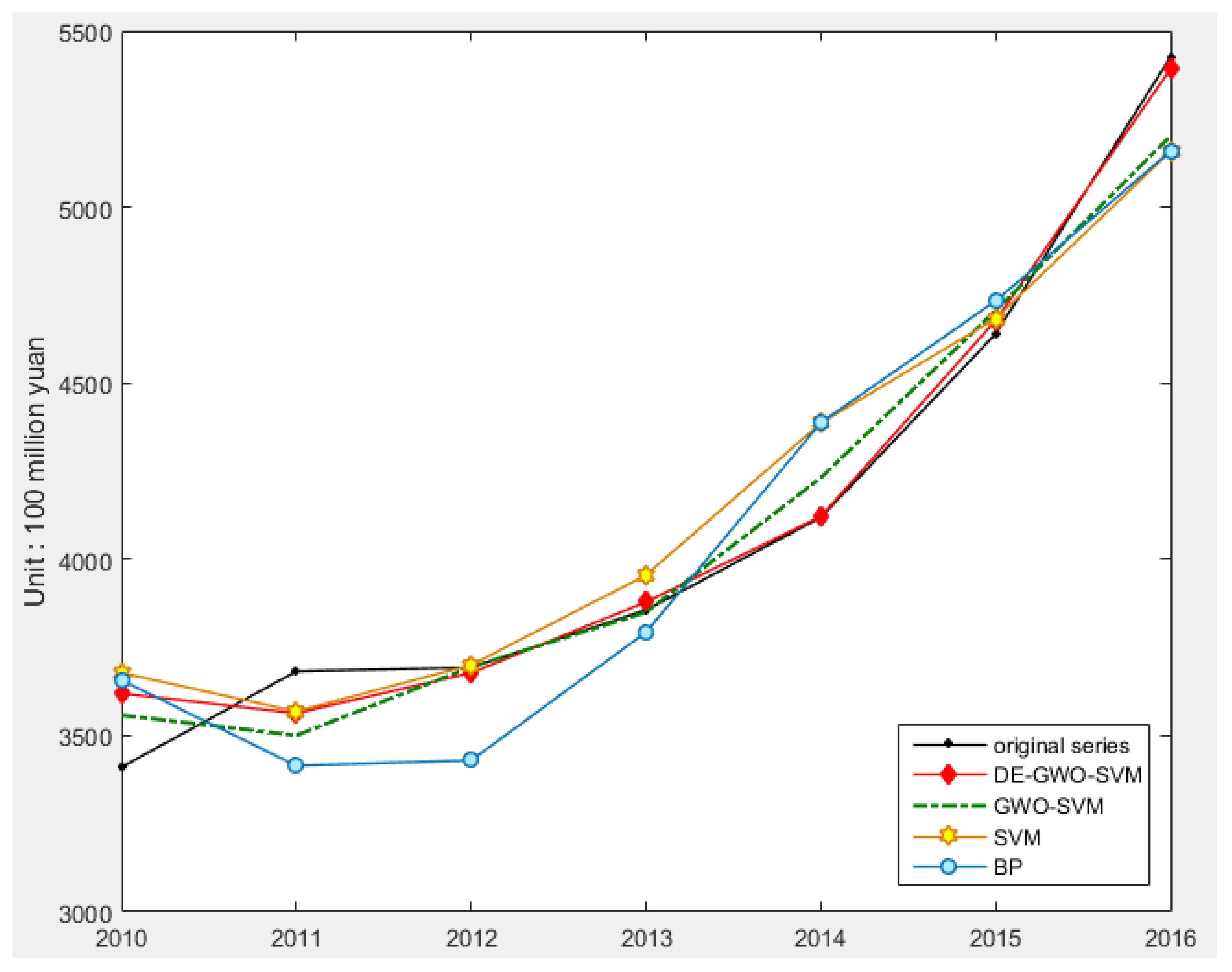
- In this article, the model of DE-GWO-SVM is proposed to predict power grid investment in China. Three algorithms—differential evolution algorithm, grey wolf optimization algorithm, and support vector machine—are combined for power grid investment forecasting. The improved combination prediction model will greatly improve the global search capability for avoiding being lost into the local optimum, which can predict the power grid investment accurately. Through empirical analysis, it is proven that the DE-GWO-SVM model has strong generalization ability and robustness in power grid investment prediction, whose prediction accuracy is better than that of GWO-SVM, SVM, and back propagation (BP) neural network.
2. Methodology
2.1. Construction of the Influencing Factors System for Power Grid Investment Forecasting
2.2. Screening of the Main Influencing Factors Based on Grey Relational Analysis
2.3. Support Vector Machine
2.4. Grey Wolf Optimization
2.5. Differential Evolution
2.6. Support Vector Machine Optimized by Differential Evolution Algorithm and Grey Wolf Optimization Algorithm
2.7. Forecasting Process
3. Empirical Analysis
3.1. Influencing Factors Screening for Forecasting Model Input
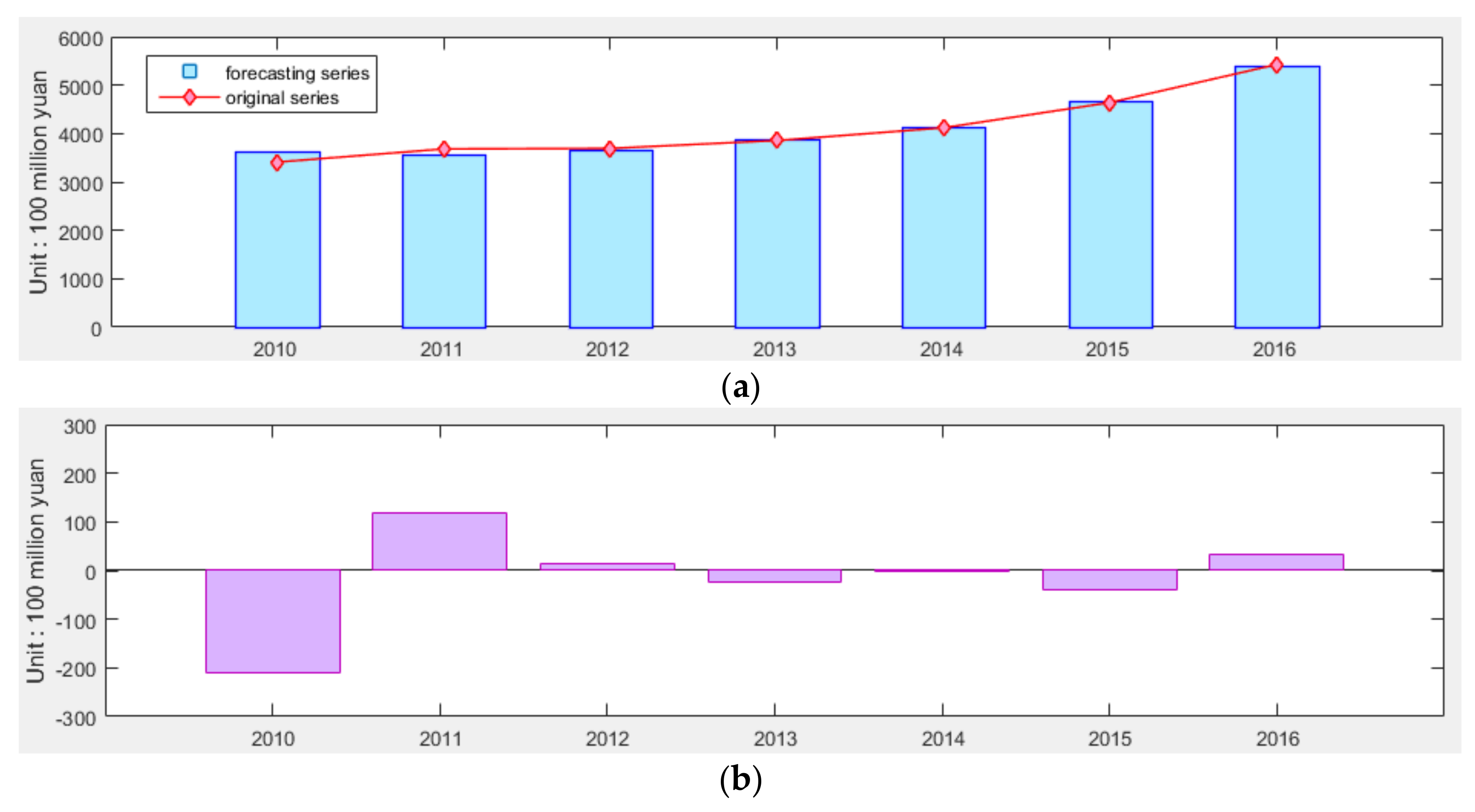
3.2. Forecasting Effect Test for DE-GWO-SVM Model
3.3. Supplementary Experiment
3.4. Forecasting of Power Grid Investment in China Based on DE-GWO-SVM Model
4. Conclusions
Acknowledgments
Author Contributions
Conflicts of Interest
Abbreviation
| Abbreviation | Full Name |
| GRA | Grey relational analysis |
| SVM | Support vector machine |
| GWO | Grey wolf optimization |
| DE | Differential evolution |
| GM | Grey model |
| BP | Back propagation |
| GWO-SVM | Support vector machine optimized by grey wolf optimization algorithm |
| DE-GWO-SVM | Support vector machine optimized by differential evolution algorithm and grey wolf optimization algorithm |
References
- Apergis, N.; Payne, J.E. Energy consumption and economic growth in Central America: Evidence from a panel cointegration and error correction model. Energy Econ. 2009, 31, 211–216. [Google Scholar] [CrossRef]
- Strachan, R.W.; Inder, B. Bayesian analysis of the error correction model. J. Econom. 2004, 123, 307–325. [Google Scholar] [CrossRef]
- Gang, L.; Wong, K.K.F.; Song, H.Y.; Witt, S.F. Tourism demand forecasting: A time varying parameter error correction model. J. Travel Res. 2006, 45, 175–185. [Google Scholar] [CrossRef]
- Zhang, X.; Pang, Y.; Cui, M.; Stallones, L.; Xiang, H. Forecasting mortality of road traffic injuries in China using seasonal autoregressive integrated moving average model. Ann. Epidemiol. 2015, 25, 101–106. [Google Scholar] [CrossRef] [PubMed]
- Chang, X.; Gao, M.; Wang, Y.; Hou, X. Seasonal autoregressive integrated moving average model for precipitation time series. J. Math. Stat. 2012, 8, 500–505. [Google Scholar] [CrossRef]
- Lin, C.S.; Liou, F.M.; Huang, C.P. Grey forecasting model for CO2 emissions: A Taiwan study. Adv. Mater. Res. 2011, 88, 3816–3820. [Google Scholar] [CrossRef]
- Hsu, C.C.; Chen, C.Y. Applications of improved grey prediction model for power demand forecasting. Energy Convers. Manag. 2003, 44, 2241–2249. [Google Scholar] [CrossRef]
- Lee, Y.S.; Tong, L.I. Forecasting energy consumption using a grey model improved by incorporating genetic programming. Energy Convers. Manag. 2011, 52, 147–152. [Google Scholar] [CrossRef]
- Lunsford, K.G. Forecasting residential investment in the United States. Int. J. Forecast. 2015, 31, 276–285. [Google Scholar] [CrossRef]
- Singh, D.P.; Dalei, N.N.; Raju, T.B. Forecasting investment and capacity addition in Indian airport infrastructure: Analysis from post-privatization and post-economic regulation era. J. Air Transp. Manag. 2016, 53, 218–225. [Google Scholar] [CrossRef]
- Chang, C.O.; Linneman, P. Forecasting Housing Investment in Developing Countries. Growth Chang. 2010, 21, 59–72. [Google Scholar] [CrossRef]
- Gupta, R. Bayesian Methods of Forecasting Inventory Investment in South Africa. S. Afr. J. Econ. 2009, 77, 113–126. [Google Scholar] [CrossRef]
- Jere, S.; Kasense, B.; Chilyabanyama, O. Forecasting Foreign Direct Investment to Zambia: A Time Series Analysis. Open J. Stat. 2017, 07, 122–131. [Google Scholar] [CrossRef]
- Zhao, H.; Lu, Y.; Li, C.J.; Ma, X. Research on Prediction to Investment Demand of Power Grid Based on Co-integration Theory and Error Correction Model. Power Syst. Technol. 2011, 35, 193–198. [Google Scholar] [CrossRef]
- Hu, B.C.; Hu, G.; Hu, C.H.; Qin, S.; Li, M.W.; Peng, C. Grid Infrastructure Investment Calculation Model Based on Gray Prediction. J. Univ. Electron. Sci. Technol. China 2013, 42, 890–894. [Google Scholar] [CrossRef]
- Fang, J.L.; Xie, Y.J.; Jin, Y.; Feng, S. Study on Forecasting Model of Power Grid Investment Scale of Electric Power Company. China High Technol. Enterp. 2016, 8, 20–21. [Google Scholar] [CrossRef]
- Russell, S.J.; Norvig, P. Artificial intelligence: A modern approach. Appl. Mech. Mater. 2010, 263, 2829–2833. [Google Scholar]
- Negnevitsky, M. Artificial Intelligence: A Guide to Intelligent Systems. Inf. Comput. Sci. 2011, 48, 284–300. [Google Scholar]
- Weng, J.; Mcclelland, J.; Pentland, A.; Sporns, O.; Stockman, I.; Sur, M.; Thelen, E. Artificial intelligence. Autonomous mental development by robots and animals. Science 2001, 291, 599–600. [Google Scholar] [CrossRef] [PubMed]
- Zhu, S.Y.; Ma, X.J.; Liang, C.Y. Application of Artificial Intelligence technology to search engine. J. Hefei Univ. Technol. 2003. [Google Scholar] [CrossRef]
- Bin, H.; Zu, Y.X.; Zhang, C. A Forecasting Method of Short-Term Electric Power Load Based on BP Neural Network. Appl. Mech. Mater. 2014, 538, 247–250. [Google Scholar] [CrossRef]
- Huang, D.Z.; Gong, R.X.; Gong, S. Prediction of Wind Power by Chaos and BP Artificial Neural Networks Approach Based on Genetic Algorithm. J. Electr. Eng. Technol. 2015, 10, 41–46. [Google Scholar] [CrossRef]
- Narayanakumar, S.; Raja, K. A BP Artificial Neural Network Model for Earthquake Magnitude Prediction in Himalayas, India. Circ. Syst. 2016, 7, 3456–3468. [Google Scholar] [CrossRef]
- Yang, J.F.; Cheng, H.Z. Application of SVM to power system short-term load forecast. Electr. Power Autom. Equip. 2004, 24, 30–32. [Google Scholar]
- Shi, X.; Huang, Q.; Chang, J.; Zhao, J. Optimal parameters of the SVM for temperature prediction. Remote Sens. GIS Hydrol. Water Resour. 2015, 368, 162–167. [Google Scholar] [CrossRef]
- Hong, W.C. Electric load forecasting by support vector model. Appl. Math. Model. 2009, 33, 2444–2454. [Google Scholar] [CrossRef]
- Ding, S.; Zhang, X.; Yu, J. Twin support vector machines based on fruit fly optimization algorithm. Int. J. Mach. Learn. Cybern. 2016, 7, 193–203. [Google Scholar] [CrossRef]
- Pan, W.T. A new Fruit Fly Optimization Algorithm: Taking the financial distress model as an example. Knowl. Based Syst. 2012, 26, 69–74. [Google Scholar] [CrossRef]
- Wang, L.; Shi, Y.; Liu, S. An improved fruit fly optimization algorithm and its application to joint replenishment problems. Expert Syst. Appl. 2015, 42, 4310–4323. [Google Scholar] [CrossRef]
- Yang, W.; Li, Q. Survey on Particle Swarm Optimization Algorithm. Eng. Sci. 2004, 6, 87–94. [Google Scholar]
- Trelea, I.C. The particle swarm optimization algorithm: Convergence analysis and parameter selection. Inf. Process. Lett. 2016, 85, 317–325. [Google Scholar] [CrossRef]
- Zwickl, D.J.; Cannetella, D.C.; Gutell, R.R.; Jansen, R.K.; Warnow, T.J. Genetic algorithm approaches for the phylogenetic analysis of large biological sequence datasets under the maximum likelihood criterion. Diss. Theses Gradworks 2006, 3, 257–260. [Google Scholar]
- Pourbasheer, E.; Riahiab, S.; Norouzi, P. Application of genetic algorithm-support vector machine (GA-SVM) for prediction of BK-channels activity. Eur. J. Med. Chem. 2009, 44, 5023. [Google Scholar] [CrossRef] [PubMed]
- Deb, K. An efficient constraint handling method for genetic algorithms. Comput. Meth. Appl. Mech. Eng. 2000, 186, 311–338. [Google Scholar] [CrossRef]
- Mirjalili, S.; Lewis, A. The Whale Optimization Algorithm. Adv. Eng. Softw. 2016, 95, 51–67. [Google Scholar] [CrossRef]
- Tharwat, A.; Moemen, Y.S.; Hassanien, A.E. Classification of Toxicity Effects of Biotransformed Hepatic Drugs using Whale Optimized Support Vector Machines. J. Biomed. Inform. 2017, 68, 132–149. [Google Scholar] [CrossRef] [PubMed]
- Qin, A.K.; Huang, V.L.; Suganthan, P.N. Differential Evolution Algorithm with Strategy Adaptation for Global Numerical Optimization. IEEE. Trans. Evol. Comput. 2009, 13, 398–417. [Google Scholar] [CrossRef]
- Liu, J.; Lampinen, J. A Fuzzy Adaptive Differential Evolution Algorithm. Soft Comput. 2005, 9, 448–462. [Google Scholar] [CrossRef]
- Abbass, H.A. The self-adaptive Pareto differential evolution algorithm. Congr. Evol. Comput. 2002, 1, 831–836. [Google Scholar]
- Saxena, P.; Kothari, A. Optimal Pattern Synthesis of Linear Antenna Array Using Grey Wolf Optimization Algorithm. Int. J. Antennas Propag. 2016, 2016, 1–11. [Google Scholar] [CrossRef]
- Vinothini, J. Grey Wolf Optimization Algorithm for Colour Image Enhancement Considering Brightness Preservation Constraint. Int. J. Emerg. Trends Technol. Comput. Sci. 2016. [Google Scholar] [CrossRef]
- Alaa, F.; Abdel-Raouf, A. Estimating the Parameters of Software Reliability Growth Models Using the Grey Wolf Optimization Algorithm. Int. J. Adv. Comput. Sci. Appl. 2016, 7, 499–505. [Google Scholar] [CrossRef]
- Jin, X.; Shao, Z.C.; Wang, S.H. A Hybrid Optimization Algorithm Based on Differential Evolution and Gray Wolf Algorithm. Sci. Technol. Eng. 2017, 17, 266–269. [Google Scholar] [CrossRef]
- Xu, D.Y.; Ding, S. Research on Short-term Prediction of Cloud Computing Resource Load Based on Improved GWO Optimization SVM. Comput. Eng. Appl. 2017, 53, 68–73. [Google Scholar] [CrossRef]
- Kuo, Y.; Yang, T.; Huang, G.W. The use of grey relational analysis in solving multiple attribute decision-making problems. Comput. Ind. Eng. 2008, 55, 80–93. [Google Scholar] [CrossRef]
- Lai, H.H.; Lin, Y.C.; Yeh, C.H. Form design of product image using grey relational analysis and neural network models. Comput. Oper. Res. 2005, 32, 2689–2711. [Google Scholar] [CrossRef]
- Huang, S.J.; Chiu, N.H.; Chen, L.W. Integration of the grey relational analysis with genetic algorithm for software effort estimation. Eur. J. Oper. Res. 2008, 188, 898–909. [Google Scholar] [CrossRef]


| Influencing Factor | Grey Relational Degree |
|---|---|
| GDP | 0.8738 |
| Industrial structure | 0.6662 |
| Population | 0.6510 |
| Urbanization rate | 0.7022 |
| Total electricity consumption | 0.8679 |
| Growth rate of electricity consumption | 0.8774 |
| Electricity sales | 0.6226 |
| Peak load of power grid | 0.6128 |
| Power transmission line length of 220 kV and above | 0.8543 |
| Power transmission line length of 110 kV and below | 0.7256 |
| Transformer capacity of 220 kV and above | 0.8733 |
| Transformer capacity of 110 kV and below | 0.7672 |
| Total profit of power grid enterprises | 0.6136 |
| Power supply load of unit power grid assets | 0.8080 |
| Electricity sales of unit power grid assets | 0.6885 |
| Electricity sales income of unit power grid assets | 0.7363 |
| Year | Power Grid Investment | GDP | Total Electricity Consumption | Electricity Sales | Power Transmission Line Length of 220 kV and Above | Transformer Capacity of 220 kV and Above |
|---|---|---|---|---|---|---|
| 1990 | 0 | 0 | 0 | 0 | 0 | 0 |
| 1991 | 0.0022 | 0.0043 | 0.0108 | 0.0164 | 0.0087 | 0.0086 |
| 1992 | 0.0058 | 0.0115 | 0.0250 | 0.0316 | 0.0216 | 0.0140 |
| 1993 | 0.0104 | 0.0232 | 0.0391 | 0.0477 | 0.0320 | 0.0204 |
| 1994 | 0.0195 | 0.0410 | 0.0550 | 0.0619 | 0.0425 | 0.0270 |
| 1995 | 0.0277 | 0.0586 | 0.0709 | 0.0767 | 0.0572 | 0.0346 |
| 1996 | 0.0302 | 0.0730 | 0.0837 | 0.0896 | 0.0692 | 0.0439 |
| 1997 | 0.0570 | 0.0839 | 0.0926 | 0.1002 | 0.0834 | 0.0529 |
| 1998 | 0.0975 | 0.0914 | 0.0984 | 0.1040 | 0.1064 | 0.0640 |
| 1999 | 0.1668 | 0.0989 | 0.1124 | 0.1172 | 0.1236 | 0.0769 |
| 2000 | 0.2483 | 0.1122 | 0.1383 | 0.1406 | 0.1432 | 0.0896 |
| 2001 | 0.2202 | 0.1268 | 0.1612 | 0.1671 | 0.1664 | 0.1072 |
| 2002 | 0.2707 | 0.1418 | 0.1933 | 0.1994 | 0.1881 | 0.1236 |
| 2003 | 0.2254 | 0.1635 | 0.2405 | 0.2494 | 0.2211 | 0.1478 |
| 2004 | 0.2284 | 0.1971 | 0.2941 | 0.3036 | 0.2600 | 0.1806 |
| 2005 | 0.2904 | 0.2323 | 0.3513 | 0.3210 | 0.3067 | 0.2211 |
| 2006 | 0.3531 | 0.2765 | 0.4191 | 0.3907 | 0.3629 | 0.2738 |
| 2007 | 0.4259 | 0.3466 | 0.4994 | 0.4679 | 0.4380 | 0.3369 |
| 2008 | 0.5270 | 0.4145 | 0.5303 | 0.5671 | 0.4927 | 0.4115 |
| 2009 | 0.7061 | 0.4553 | 0.5741 | 0.6117 | 0.5652 | 0.4984 |
| 2010 | 0.6247 | 0.5435 | 0.6759 | 0.7330 | 0.6478 | 0.5675 |
| 2011 | 0.6754 | 0.6486 | 0.7707 | 0.8376 | 0.7003 | 0.6337 |
| 2012 | 0.6774 | 0.7191 | 0.8202 | 0.8801 | 0.7553 | 0.7378 |
| 2013 | 0.7077 | 0.7947 | 0.8912 | 0.9271 | 0.8237 | 0.8077 |
| 2014 | 0.7567 | 0.8619 | 0.9253 | 0.9666 | 0.8841 | 0.9018 |
| 2015 | 0.8537 | 0.9241 | 0.9303 | 0.9644 | 0.9405 | 0.9206 |
| 2016 | 1 | 1 | 1 | 1 | 1 | 1 |
| Parameters | Values |
|---|---|
| The regularization parameter search range | 0.1, 200 |
| The the radial basis kernel function parameter search range | 0.01, 20 |
| Population size | 20 |
| Maximum iteration number | 200 |
| Crossover probability | 0.2 |
| The scope of the zoom factor | 0.2, 0.8 |
| Model | MAPE (%) | RMSE (Billion Yuan) | MAE (Billion Yuan) |
|---|---|---|---|
| DE-GWO-SVM | 1.70 | 9.36 | 6.31 |
| GWO-SVM | 2.54 | 13.22 | 10.58 |
| SVM | 3.73 | 18.51 | 15.25 |
| BP | 5.25 | 22.63 | 21.01 |
| Model | MAPE (%) | RMSE (100 Million Yuan) | MAE (100 Million Yuan) |
|---|---|---|---|
| DE-GWO-SVM | 0.13% | 0.17 | 0.10 |
| GWO-SVM | 0.73% | 0.68 | 0.43 |
| SVM | 3.29% | 2.16 | 2.16 |
| BP | 6.00% | 3.97 | 3.96 |
© 2018 by the authors. Licensee MDPI, Basel, Switzerland. This article is an open access article distributed under the terms and conditions of the Creative Commons Attribution (CC BY) license (http://creativecommons.org/licenses/by/4.0/).
Share and Cite
Dai, S.; Niu, D.; Han, Y. Forecasting of Power Grid Investment in China Based on Support Vector Machine Optimized by Differential Evolution Algorithm and Grey Wolf Optimization Algorithm. Appl. Sci. 2018, 8, 636. https://doi.org/10.3390/app8040636
Dai S, Niu D, Han Y. Forecasting of Power Grid Investment in China Based on Support Vector Machine Optimized by Differential Evolution Algorithm and Grey Wolf Optimization Algorithm. Applied Sciences. 2018; 8(4):636. https://doi.org/10.3390/app8040636
Chicago/Turabian StyleDai, Shuyu, Dongxiao Niu, and Yaru Han. 2018. "Forecasting of Power Grid Investment in China Based on Support Vector Machine Optimized by Differential Evolution Algorithm and Grey Wolf Optimization Algorithm" Applied Sciences 8, no. 4: 636. https://doi.org/10.3390/app8040636
APA StyleDai, S., Niu, D., & Han, Y. (2018). Forecasting of Power Grid Investment in China Based on Support Vector Machine Optimized by Differential Evolution Algorithm and Grey Wolf Optimization Algorithm. Applied Sciences, 8(4), 636. https://doi.org/10.3390/app8040636