Article

Predicting Output Power for Nearshore Wave Energy Harvesting

Department of Information and Communications Engineering, Myongji University, 116 Myongji-ro, Yongin, Gyeonggi 17058, Korea
*
Author to whom correspondence should be addressed.
Appl. Sci. 2018, 8(4), 566; https://doi.org/10.3390/app8040566
Submission received: 22 February 2018 / Revised: 15 March 2018 / Accepted: 3 April 2018 / Published: 5 April 2018
(This article belongs to the Special Issue Applications of Artificial Neural Networks for Energy Systems)

Abstract

:
Energy harvested from a Wave Energy Converter (WEC) varies greatly with the location of its installation. Determining an optimal location that can result in maximum output power is therefore critical. In this paper, we present a novel approach to predicting the output power of a nearshore WEC by characterizing ocean waves using floating buoys. We monitored the movement of the buoys using an Arduino-based data collection module, including a gyro-accelerometer sensor and a wireless transceiver. The collected data were utilized to train and test prediction models. The models were developed using machine learning algorithms: SVM, RF and ANN. The results of the experiments showed that measurements from the data collection module can yield a reliable predictor of output power. Furthermore, we found that the predictors work better when the regressors are combined with a classifier. The accuracy of the proposed prediction model suggests that it could be extremely useful in both locating optimal placement for wave energy harvesting plants and designing the shape of the buoys used by them.

1. Introduction

Although wave energy harvesting technology was proposed as early as the late Eighteenth Century, in recent years, it has attracted particular attention as a potentially viable source of renewable energy [1]. Renewable energy, a central component of efforts to reduce the use of natural resources and to mitigate climate change, is currently generated from several sources, including solar, wind, tides, water, biomass and waves, most of which are rooted in solar radiation. Despite wave energy’s noteworthy advantages, including its considerable power density, low environmental impact, relative consistency, potential predictability and the low costs of operation and maintenance of installations, it has not been as widely explored as other renewable energy sources [2,3].
Wave energy is an especially promising alternative energy source for South Korea, whose limited natural resources and resistance to adding nuclear power to its energy mix makes the county entirely dependent on imports to meet its energy demands [4]. The government’s commitment to expanding the use of renewable energy through its Renewable Portfolio Standard (RPS), which mandates that energy producers include a minimum portion of their installed capacity in the form of energy generated from renewable sources [5], has added particular impetus to the development of effective and efficient alternative sources.
In response to these factors, the South Korean company INGINE has recently developed a new device for harvesting wave energy close to shore. A nearshore location can resolve the energy transmission problems of conventional wave energy plants that are far from areas of energy consumption. INGINE’s device is composed of floating buoys located less than 100 m from the coast that capture wave energy and transfer it to power generating units onshore. The new device increases electric power generation efficiency by storing a portion of the transferred power and utilizing it during periods when energy demand exceeds energy production [6]. The ability to predict the output of such devices is key to determining the optimal location, size and configuration of power plants. In this paper, we discuss our development of a wave power predictor for the INGINE device.

1.1. A Summary of Wave Energy Conversion

Wave energy conversion is realized with the aid of a wave energy converter (WEC), a device that captures the energy inherent in the motion of waves and transforms it into electricity. WECs can be categorized according to their location (relative to the shoreline), their operational principle and their directional characteristics. Based on its distance from the shoreline, a WEC is categorized as either onshore, nearshore or offshore, with potential energy generation and difficulty of installation increasing in direct proportion to distance from the shore.
In terms of operational principle, WECs are divided into four types [1]: oscillating water columns, overtopping devices, submerged pressure differential devices and oscillating wave surge converters. Oscillating water columns use waves to compress and expand air to rotate an air turbine that produces electricity. Overtopping devices capture the movement of the tides and waves and coverts it into potential energy by lifting the water to a higher-level reservoir, where it is used to drive a hydro-pump to produce electricity [7]. Submerged pressure differential devices are submerged point absorbers that utilize the pressure differential above the device between wave crests and troughs. Oscillating wave surge converters are composed of a hinged deflector positioned perpendicular to the wave direction that moves back and forth, exploiting the horizontal particle velocity of the wave.
On the basis of directional characteristics, WECs can be categorized as attenuators, point absorbers and terminators. Attenuators lie parallel to the predominant wave direction and ride the waves. Point absorber devices absorb wave energy in all possible directions through the wave’s multi-directional movement. Terminator WECs absorb the wave energy in one direction only [8].
In addition to integrating renewable energy systems in the main power grid, maximizing the yield from these systems is important. Since the performance of such systems is influenced by non-human factors, such as environmental conditions, accurate prediction of output power is essential in determining the optimal location, size and configuration of the power plants. This study focuses on developing a prediction model for nearshore WECs that can help to determine both the optimal location and the optimal shape of the buoy.

1.2. Methods for Predicting Power Generation

There are numerous methods for predicting the power generated from renewable energy sources. Support vector machines (SVMs) have been utilized to predict solar power by analyzing four years of historical satellite images [9]. The images were processed to extract a large number of input and output datasets for the SVM algorithm. The prediction model performed better than conventional time series methods. Fuzzy models that developed a prediction model from the relationship between the wave height and the power generation were proposed for forecasting electric power generation from ocean waves in Thailand [10]; the dataset for this experiment was collected from a video camera and a multimeter connected to the load. In the fuzzy modeling, the wave height is the input (cm), and electric power is the output (Watt). The video camera and a PVC pipe with a scale were used to measure the wave height, and a multimeter connected to a load of 300 W was used to measure the output power. Machine learning was used to forecast output power of photovoltaic (PV) systems based on four classes of weather condition [11]: clear sky, cloudy, foggy and rainy. Weather forecasting data and actual historical power output were used to develop a prediction model, which was tested on a real PV station; these proved to be effective.
A comprehensive survey of machine learning applications in supporting renewable energy generation and integration that was presented by Perera, Aung and Woon [12] covered different techniques used to predict the output power from solar, wind and hydropower sources. Based on these studies, we can generalize that machine learning algorithms can be used to develop effective prediction models for renewable energy systems.
There are several mechanisms to predict output power from wave energy converters including spectral analysis methods. However, the goal of this study is to establish a new method using machine learning algorithms, which can estimate the average power based on the movement data of the buoy. In this paper, we discuss our development of a wave power prediction model for the nearshore WEC made by INGINE. The model exploits machine learning algorithms to predict electric power generation from the movement of the buoys. The movement is monitored by an offshore module consisting of a tri-axial MPU6050 gyro-accelerometer sensor, a microcontroller and wireless transmitter that is attached to the buoy. This transmitter communicates with an onshore module that comprises a microcontroller and a wireless receiver. We analyzed the relation between the movement of buoys and the power generated by the WEC using machine learning algorithms, and we evaluated whether the model works for forecasting electric power generation. To this end, we applied several preprocessing techniques before classifying the collected data using supervised learning algorithms. We compared the performance of three classifiers: support vector machine (SVM), random forest (RF) and artificial neural network (ANN). The collected data were segmented, and each segment was labelled as weak, mild or strong in accordance with the amount of power generated. Based on the classification and the segmented data, we developed a regression model for the data to predict the power generation.
Section 2 describes the working principle of the wave power harvesting device developed by INGINE. Section 3 explains the proposed approach and the experimental procedures. In Section 4, we explain the experiments that were conducted. Section 5 deals with the simulation result and includes a discussion of the work. In the final section, we offer our concluding remarks.

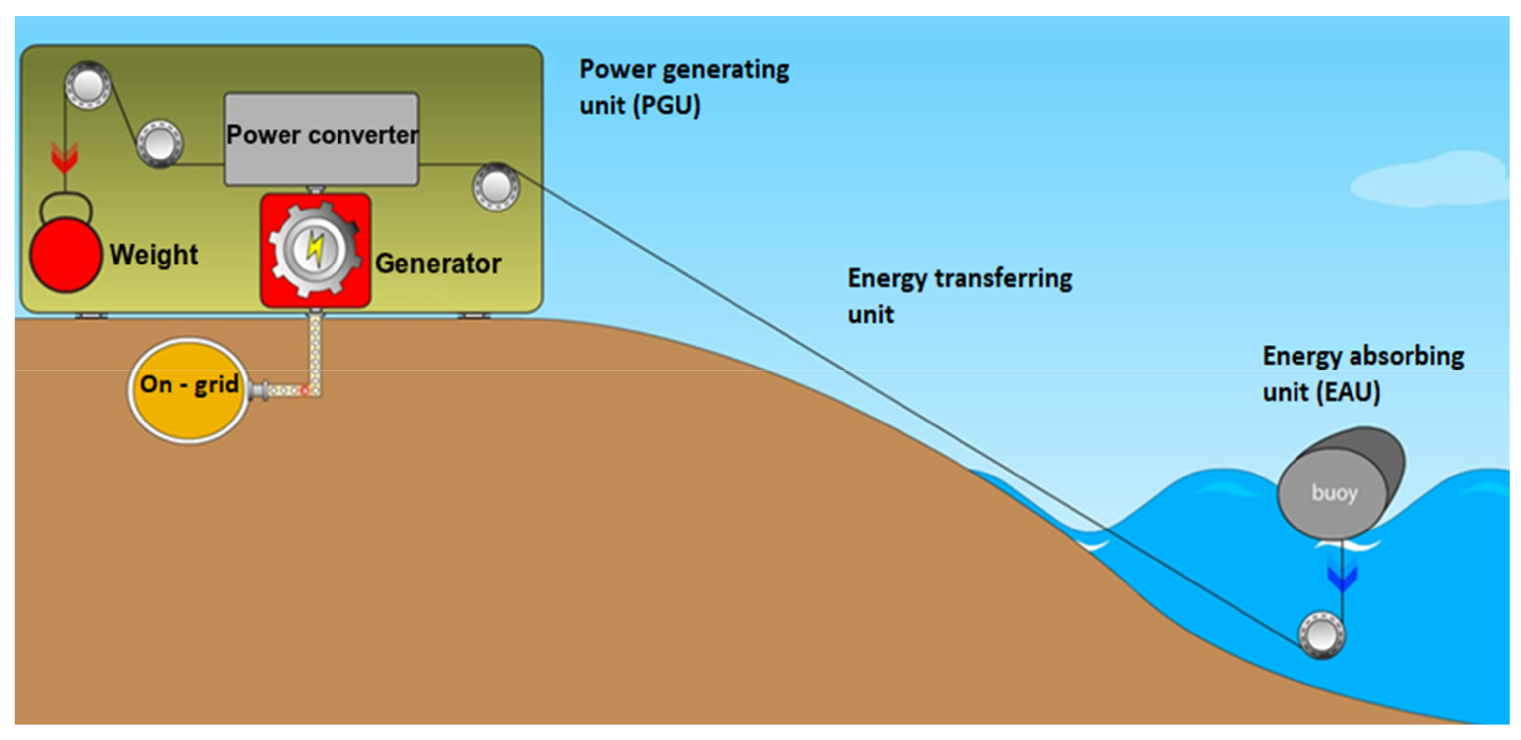
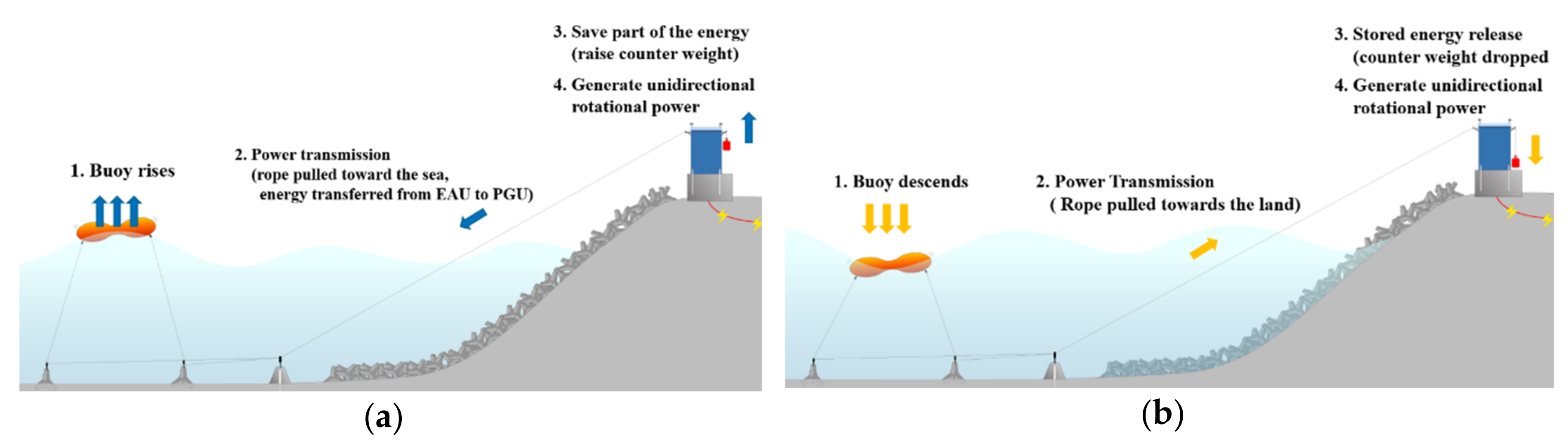
2. Wave Energy Generation
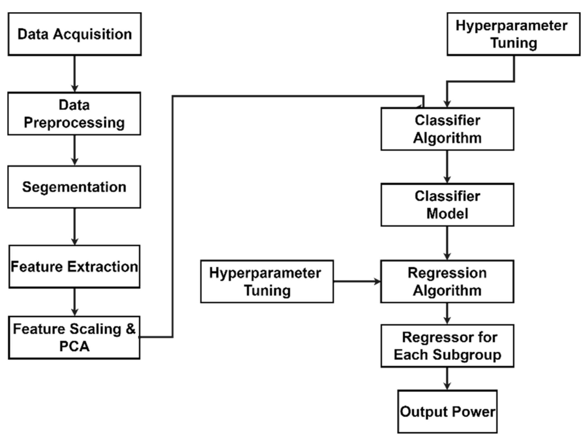
Nearshore wave energy converters are installed in waters of moderate depth and only a few hundred meters from the coastline, thus offering the advantages of lower construction and maintenance costs than deep-water devices. INGINE’s new system takes advantage of the nearshore location and adopts an innovative method for generating power using the whole range of wave movements, even in shallow waters [6].
Figure 1 shows the schematic diagram of the system. The system is composed of two main building units: the energy absorbing unit (EAU) and the power generating unit (PGU). The EAU is a floating buoy, located approximately 80 m from the shoreline, anchored to the pulley located at the seabed depth of 4 m, which is connected to the onshore PGU by three ropes, the tension of which is balanced by counterweights. The buoy is able to move within a limited range in any direction in response to wave motion. When the buoy rises, at least one of the connecting ropes pulls to the water side, and the kinetic energy from the motion is transferred to the PGU [13]. The opposite ends of the ropes connecting the buoy to the power converter are attached to a drum, where the linear reciprocating motion is converted into rotary motion through the process of winding and unwinding the rope on the drum. A one-way clutch installed inside the drum ensures that the shaft connected to the generator always rotates in one direction. The wave energy recovered by the EAU is thus transferred to the PGU through the reciprocating motion of the ropes, which is further converted into the one-directional rotary motion of a generator turbine. In this system, energy transfer from the water side to the land side occurs only when the buoy rises; consequently, the WEC generates power only when the ropes are pulled by the rising buoy. On the other hand, when the buoy descends, the counterweight attached to the other end of the rope maintains the tension on the rope and ensures that the buoy stays in its designated position. The direction of movement of the buoy and the rope is indicate by the arrows in Figure 2.
This WEC increases the power generating efficiency by storing the energy transferred from the water side. According to Sung, Kim and Lee [6], the PGU uses a portion of the transferred energy to rotate the output shaft of the generators and a portion as stored potential energy. Thus, the system can compensate for fluctuations in wave strength by using the stored energy. As Figure 2 illustrates, the power-transmitting ropes are wound and unwound as the buoy moves up and down, respectively. As a result, the PGU generates electric power continuously, and structural stability is maintained regardless of any external force exerted by the waves.

3. Methods

This section describes the methods used to obtain the data of the buoy to reach a final characterization of the wave. A wave’s energy generating potential at a specific point on the wave can be roughly measured by the height, period and direction of the wave at the point. However, for example, waves of the same height may produce different behaviors in the buoy and in turn generate different amounts of electric power. Therefore, it is necessary to monitor the movement of the buoy and to associate the movement with the electric power that is generated. Assuming we can obtain clear relationships between them, we are able to predict the power generation from the movement of the buoy.

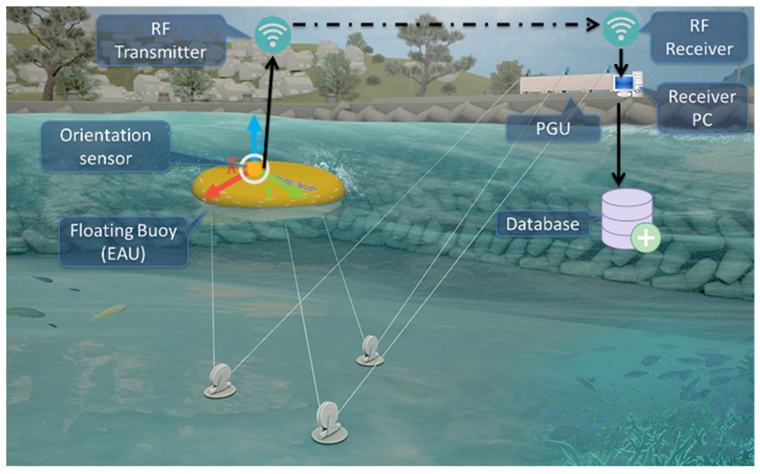
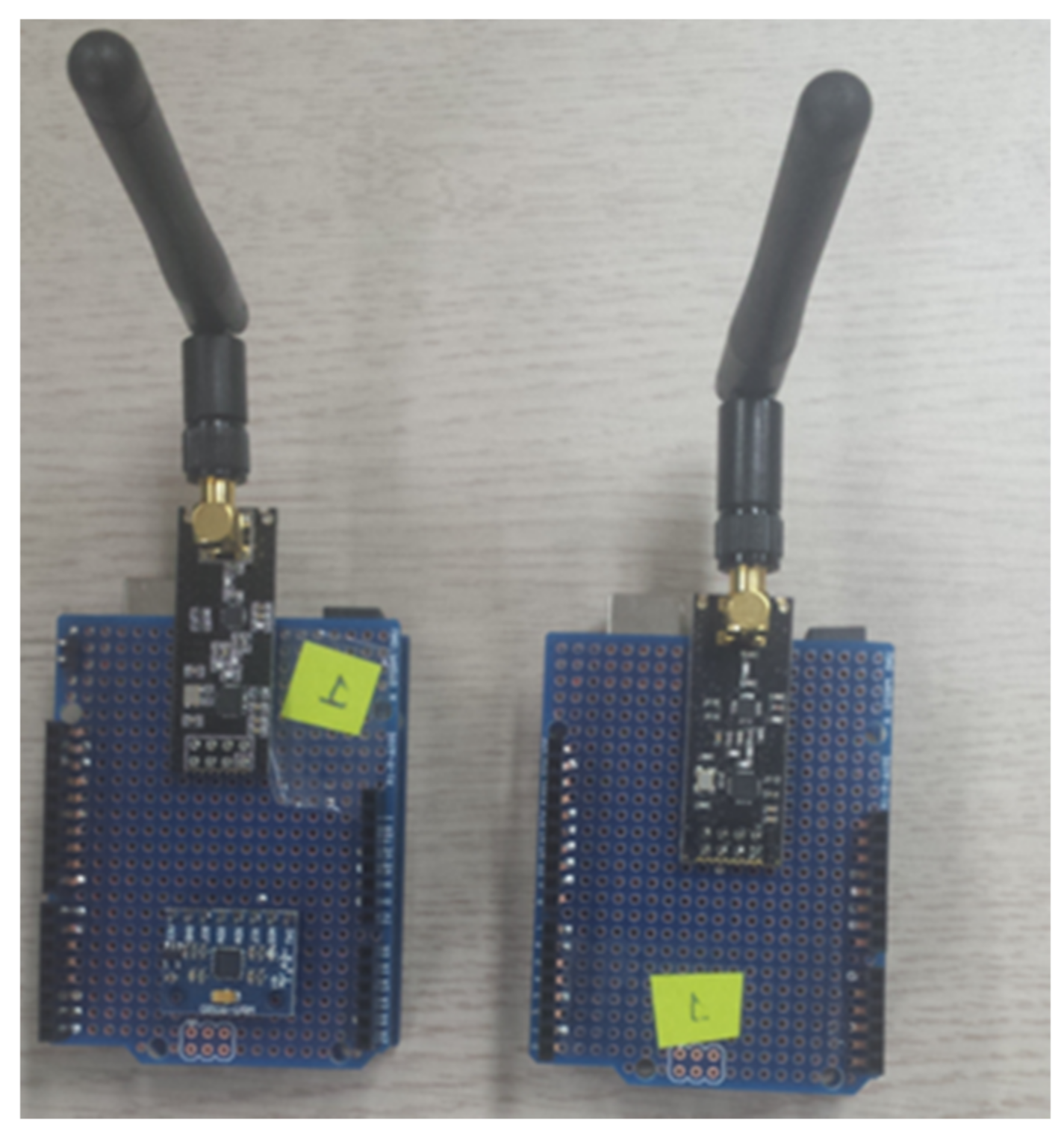
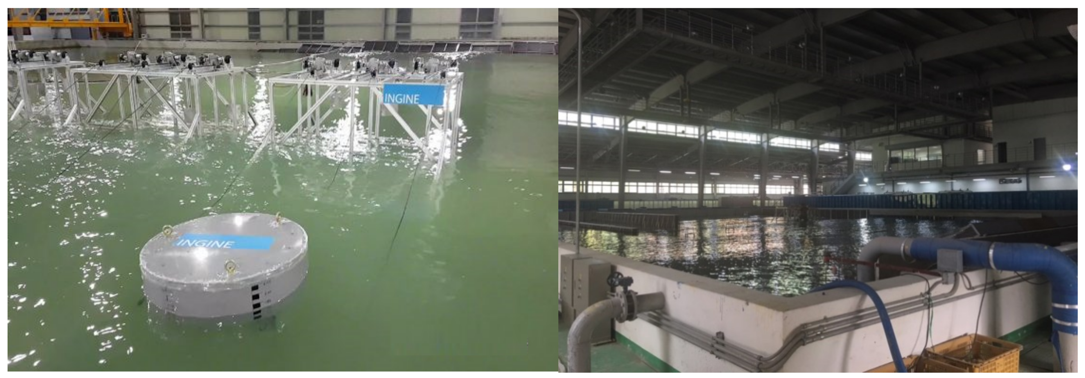
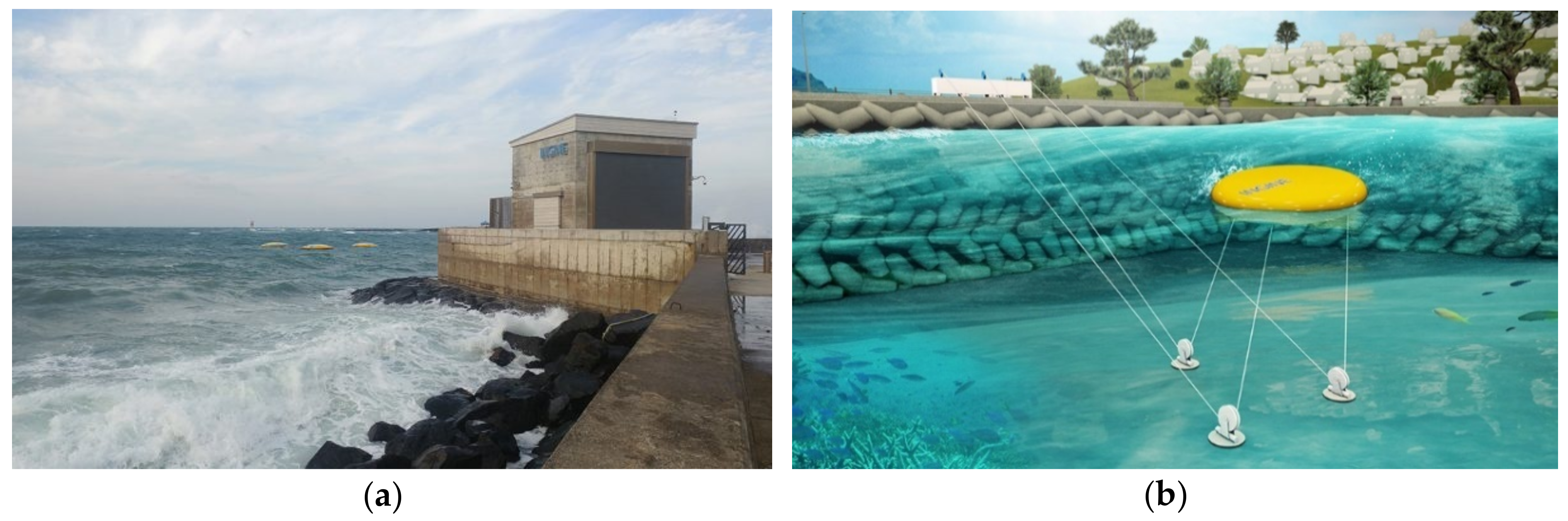
3.1. Data Collection

The data from the floating buoy were collected by an installation on the buoy and were transmitted to a computer and stored in a database for further analysis, as shown in Figure 3. The data consist of three accelerations and three angular velocities along the x, y and z axes, respectively. Thus, the dataset is composed of six time series data.
Wireless data transmission is accomplished with the transmitter and receiver module. The transmitter is composed of an MPU6050 tri-axial gyro-accelerometer sensor, an NRF2401 2.4-GHz transceiver and an Arduino microcontroller. The MPU6050 senses the accelerations and the angular velocities, and these data are transmitted by the NRF2401 transceiver shown in the left of Figure 4. Both are controlled by an Arduino microcontroller. The receiver module has an NRF2401 transceiver moderated by an Arduino. The gyro-accelerometer sensor, MPU6050, provides six time series data that represent the orientation of the floating buoy at a specific time. This dataset includes linear acceleration and angular velocity, as previously noted. The NRF2401 transceiver enables the data to be transmitted from the water side to the computer side. The transceiver can cover more than one hundred meters, which makes it suitable for nearshore applications [14]. Figure 4 shows the data collection module.

3.2. Data Segmentation and Feature Selection

Features serve to describe the characteristics of the source in machine learning. Feature extraction is used to obtain new features that are extracted from the original data. These new features are fewer in number, but are still effective in describing the source. Therefore, it is necessary to find quality features from the transmitted data to characterize the wave.
The data received from the buoys contain the information of the wave for energy harvesting. It is usually corrupted by noise or outliers, so it must go through preprocessing procedures to filter out abnormalities. Noise occurs in all measurements; outliers may include recording errors caused by faulty operation in the sensor, for example. In this study, we employed a moving average filter.
The raw time series data from the MPU 6050 contain angular velocities ( ω x , ω y , ω z ) and accelerations ( α x , α y , α z ). Since these values represent movement information of the buoy at a specific moment, they are not viable as a feature set for machine learning algorithms. We segmented the dataset into a certain size to use as a feature. Windowing approaches are normally used for segmentation, but no clear consensus exists on which window size should be preferably employed [15]. One reliable clue is the period of the wave. It is obvious that the segmented data correspond to at least more than one period to carry the characteristics of the wave. The longer data seem to be the better representation, but it in turn becomes a burden for computation and should be restrained. In this work, we chose the size of data to be at least one period or longer.
Feature selection has a significant impact on the performance of the prediction model and the computation time of the system. Therefore, features should capture important information of the data [16]. The angular velocities and accelerations are orientation-sensitive data, but the associated power generation may be independent of orientation. It is necessary to generate new orientation-insensitive variables from the angular velocities and accelerations, such as the magnitudes of accelerations (α) and angular velocities ( ω ). This magnitude equals the Euclidean distance from the origin. From the eight variables including the original six measurements and two magnitudes from segmented dataset, we derived sixteen new statistical variables that can characterize the windowed interval. The new features consist of the means of the accelerations ( μ α x ,   μ α y ,   μ α z ,   μ α ), the means of the angular velocities ( μ ω x ,   μ ω y ,   μ ω z ,   μ ω ), the variances of the accelerations ( σ α x 2 ,   σ α y 2 ,   σ α z 2 ,   σ α 2 ) and the variances of the angular velocities ( σ ω x 2 ,   σ ω y 2 , σ ω z 2 , σ ω 2 ).
Feature scaling is a process of standardizing the range of independent variables [17]. Since the features derived from the dataset can have various ranges of values, applying the features without standardization to a machine learning algorithm would yield erroneous outcomes. Among the varieties of feature scaling techniques, we used the standard scaling approach in this paper. Standard scaling, often called Z-score normalization, transforms our feature into a standard normally-distributed variable (Gaussian with a mean of zero and a unit standard deviation). In this approach, all the feature values are scaled up or down using the following equation:
x = ( x x ¯ ) σ
where x is the numeric value of data and x ¯ and σ represent the mean and standard deviation of x, respectively.

3.3. Principal Component Analysis

Principal component analysis (PCA) is a statistical procedure that uses an orthogonal transformation. As a result of applying PCA, a set of data of possibly correlated variables is converted to a set of values of linearly uncorrelated variables called principal components. The first component has the largest variance, and each following component in turn has the largest variance among the rest. Therefore, it is expected that only the first few principal components are able to express the data in a new set of orthogonal coordinates approximately, but quite accurately. As a consequence, PCA decreases the dimension of the data and thus reduces the computation time [18]. In this study, we applied PCA to the dataset, and we selected features that can explain 90% of the total variance. As a result, the new dataset consisted of more efficient and representative variables. We applied PCA in all of the experimental cases including the real wave power station experiment.

3.4. Machine Learning Algorithms

Machine learning is a field of study that gives computers the ability to learn from data without being completely programmed [19]. In this study, we used support vector machine (SVM), random forest (RF) and artificial neural networks (ANN) to develop a prediction model for the nearshore WEC.
SVM is designed to find a separating hyperplane that can classify the input values into several class labels with minimum classification error and maximum separation. It can be applied to regression, classification and pattern recognition problems [20]. RF is an ensemble approach that incorporates multiple decision trees to generate accurate models. In standard trees, each node is split using the best split among all variables. In RF, each node is split using the best among a subset of predictors randomly chosen at that node. This slightly counterintuitive strategy performs well compared to many other classifiers and is robust against overfitting [21]. Artificial neural networks are mathematical models whose structure and tuning procedure have some analogies with brain neural networks and their learning process. ANNs represent a nonlinear mapping between an input vector and an output vector. They consist of a system of interconnected neurons. Neurons are interconnected by weights. The output signals from each node are a function of the sum of the inputs to the node modified by a simple nonlinear transfer function called the activation function [22]. ANN has been applied to several real-world applications including power predictions. In this study, we thoroughly analyzed the performance of the three algorithms listed above regarding nearshore wave power prediction.
In this study, we divide the data obtained from buoy into two parts, one for training and the other for testing. From the buoy, we obtained data that are segmented into several pieces as D1, D2, ..., and Dn. Simultaneously, there were the corresponding average power data, which were also divided into pieces as P1, P2, …, and Pn. Using the pairs (D1, P1), (D2, P2), …, (Dm, Pm) where m < n, we trained ANN, RF and SVM. Then, the trained algorithms can predict (estimate) the output ( P ^ m + 1 , , P ^ n ) with the input (Dm+1, …, Dn). Since we have the actual average power Pm+1, …, Pn, we can compare these actual values with the predicted values to evaluate the ML algorithms.
In applying machine learning algorithms, there are some parameters in the algorithms that should be set by the user before the learning process begins. We call these hyperparameters. To obtain the optimal performance of the ML algorithm, it is necessary to find the proper hyperparameters, a process called hyperparameter tuning [23]. The task varies in accordance with the ML algorithms. We applied a tenfold cross-validated grid search on the tunable parameters of the models. First, we applied a general search with a wider range of the parameters. Then, we applied a finer grid search in the neighborhood of the first selection to find the best values for the hyperparameters.
In this paper, SVM, RF and ANN were chosen to address the problem. For SVM, the main task was to select an appropriate kernel that fits the problem to find the optimal values for the gamma and penalty parameter [24]. The parameter gamma is the inverse of the radius of influence of samples selected by the support vectors. If gamma is too small, the model is constrained and thus might be unable to capture the complexity of the data. On the other hand, if gamma is too large, it may lead to overfitting. The penalty parameter trades off misclassification of training examples against the simplicity of the decision surface. The main parameters tuned for the RF were the number of trees, the number of features and the criterion, which is a function to measure the quality of a split [25]. Similarly, for ANN, the number of neurons, the number of layers, the size of the batch and the number of epochs were fine-tuned.

3.5. Architecture of the Proposed Approach

Figure 5 summarizes the flow of the proposed procedure described in this section. Data collection occurs as the movement of the buoys was measured and sent to the computer onshore. Then, these data were filtered out to remove abnormalities before the data were segmented with a properly-sized window. As a result, eight time series data were derived from the window. We calculated two statistical variables, mean and variance, from the data of each time series so that they served as features. These features were standardized, and PCA was applied to these scaled features to reduce their dimension. Before developing prediction models based on ML algorithms, hyperparameter tuning was done with each algorithm. To check the validity of the models, the dataset was split into training and testing sets. We used 70% for training and 30% for testing the models.
Regression is performed to obtain the forecasting values of power generation. This is done in two ways: with a classifier and without a classifier. Regression with a classifier yields estimates using the classification result in the previous step. Depending on the result, there are three types of models available for regression. Classification has a positive effect on improving the accuracy of regression models [26]. Intuitively, the subsequent regression can narrow the interval of the estimate so that the prediction error could be smaller. Regression without a classifier was employed in only one model. Therefore, the resultant estimate cannot be as accurate as one with a classifier, in general, but it can yield a better result in case an incorrect classification is highly likely.

4. Experiments

We conducted experiments at two different sites. One experiment was run in a wave tank simulator where the environment was controllable. The other was run in an actual wave power harvesting plant for five days, which showed a wide enough range of output power to classify waves into three levels of power generation.
The wave tank simulator was located at Chonnam University, Yeosu, South Korea. The purpose of this experiment was to evaluate the feasibility of the proposed method before it was deployed in the actual site. The wave tank simulator was 50 m wide, 50 m long and 1.5 m tall, and it had the capacity to generate waves with periods ranging from 0.5–4 s and a maximum height of 60 cm. A WEC reduced to 1/20 of its original size was used at the site, as shown in Figure 6. In the experiment, we also used a smaller buoy, which had a radius of 1 m and a height of 0.5 m.
In the wave tank experiment, we attached the data collection module to the top of the buoy. For the simulation, we generated three types of regular waves: weak, mild and strong. Since waves generated in the tank are smaller than actual offshore waves, we scaled down the wave height and the period by a factor of 20. Table 1 shows the values for actual waves and the adjusted values for the waves in the wave tank. The three cases in the left column of the table represent the wave patterns for strong, mild and weak, respectively. The average powers in the table correspond to power generated for each case. The experiment for each case was conducted for 5 min without altering the experimental setup.
The second experiment site was located at Bukchon in Jejudo, the largest island in South Korea. We installed the data collection module on top of the yellow buoy and the receiver inside the power plant building located on the shoreline (see Figure 7). The distance between the buoy and the building was approximately 80 m. The incoming data were continuously monitored and recorded throughout the experiment. We segmented the data with several sizes and observed how the performance varied.

5. Results and Discussion

5.1. Evaluation Metrics

Evaluation metrics evaluate the quality of a model’s performance. For this study, we needed to quantify the validity of a regression model. We used mean absolute error (MAE), mean squared error (MSE) and R2 for the metrics of the regression. These metrics find the difference between actual values and predicted values. The definition of the evaluation metrics is shown in Table 2.

5.2. Wave Tank Experiment

As explained in Section 4, three waves with different periods and heights were generated, and the movement of the buoy was monitored by a data collection module. In order to estimate the power generation, classification was performed beforehand so that the corresponding regression model could be applied. The detailed results of data segmentation and prediction are presented below.

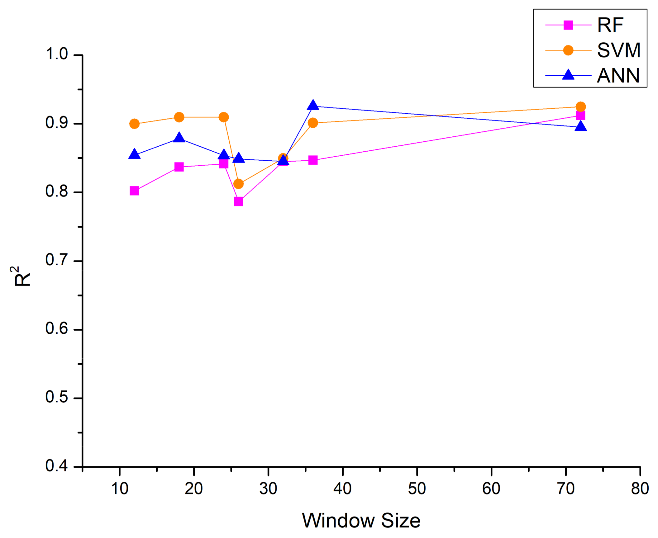
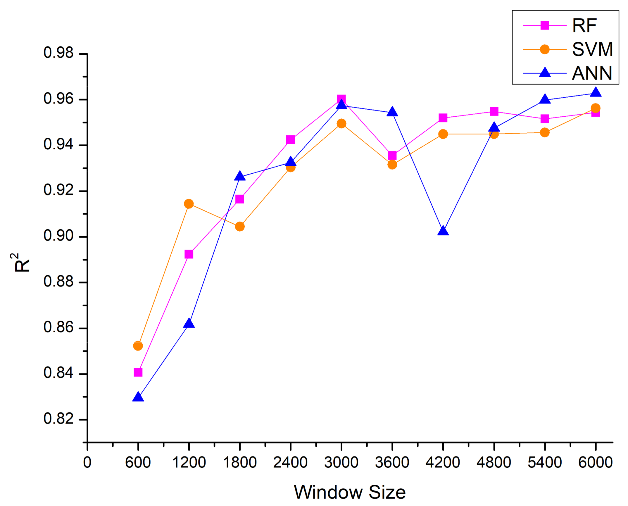
5.2.1. Data Segmentation

To carry out classification and regression, it was necessary to segment data for the analysis because the data were dynamically changing. We adopted a windowing approach; however, the appropriate size of the window should be found by trial and error [15]. To find the most appropriate window size, we performed several experiments with different window sizes by applying three types of ML algorithms: RF, SVM and ANN.
The data in the wave tank experiment were obtained with a sampling frequency of 12 Hz. We considered seven window sizes: 12, 18, 24, 26, 32, 36 and 72, which corresponded to window durations of 1, 1.5, 2, 2.16, 2.67, 3 and 6 s, respectively. Table 3 shows the numbers of the training and testing datasets. It is obvious that the window size dictated the number of samples because the total number of available data is constant.
Figure 8 shows the performance depending on the various window sizes defined in Table 3. The best result for the prediction model was found when the window size was 72. With this, the number of training datasets was 111 and that of testing datasets was 48. We used this window size (72) for the remainder of the wave tank experiment.

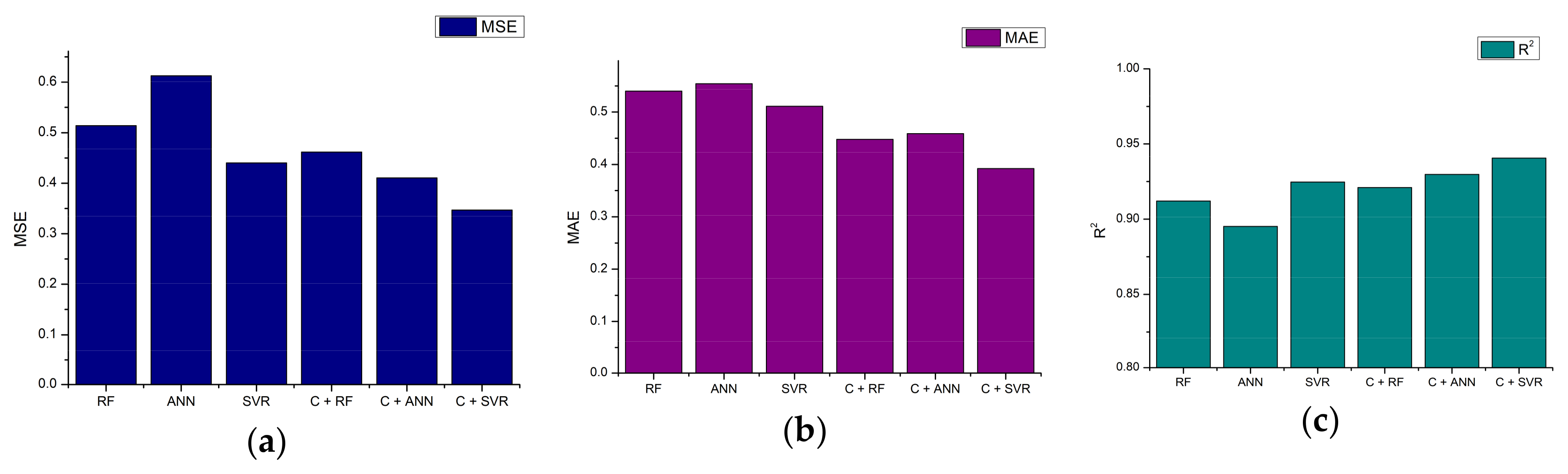
5.2.2. Output Power Estimation

To predict the output power, it is necessary to apply classification and regression steps after preprocessing the input data up to the hyperparameter tuning, as shown in Figure 5. For this experiment, we segmented the data into a group of 72 samples; the number of training and testing samples were 111 and 48, respectively, as noted in the previous section.
The experiment was also designed to identify the best predictor for waves among six types of predictors, which are grouped into two. The first group, containing three types, used ANN, RF and SVM algorithms as regression models. The second group, containing the remaining three types, were the prediction models in which the regressor was preceded by the classifier. For instance, the predictor based on ANN performed classifications and then chose the ANN regression model depending on the result of the classification. In Figure 9, we denote it as C + ANN. The other types can be expressed as C + RF and C + SVR (support vector regressor). These notations hold the same for the other figures in the manuscript. The performances of the proposed systems were analyzed using the mean absolute error (MAE), mean squared error (MSE) and R2 metrics.
Regardless of the metrics used, it is clear that the second group, which used a classifier and a regressor together, outperformed the first group without a classifier, as shown in Figure 9. The result of the first group indicates that SVR is the best in two metrics and ANN in one metric, and RF shows the least favorable result. Among the second group, all of the algorithms resulted in a similar amount of error with a slight difference. The predictor based on the SVR model (C + S VR) had the highest R2 score and the minimum MSE and MAE error values. We selected this model as the prediction model for our proposed approach.

5.3. Actual Wave Energy Harvesting Plant Experiment

Similar to the wave tank study, we conducted two distinct experiments on the collected dataset. Each sample in the dataset was labeled either strong, mild or weak in accordance with the output power. Wave patterns that generated more than 50% of the maximum output power were considered strong. When the power was between 10% and 50% of the maximum output, the wave pattern was labeled mild. If it was less than 10%, it was labeled weak. The results of the experiments are presented below.

5.3.1. Data Segmentation

Ocean waves, unlike waves in a tank, are irregular in nature and have a wider frequency spectrum. To handle the frequency variation, we adopted wider window sizes so that low-frequency components could be considered. The data were collected at 10 Hz, and the sizes of the windows were 600, 1200, 1800, 2400, 3000, 3600, 4200, 4800, 5400 and 6000 samples, as shown in Table 4.
We used three regressors to investigate the effect of the window size on the prediction accuracy. Figure 10 illustrates that the regressors tended to perform better as the window size increased. The maximum R2 value, 0.962, was obtained at the window size of 6000 samples by the ANN regressor.
Since the performance of the prediction models varies with the nature of the dataset and complexity, we have noticed that the prediction accuracy of the models fluctuates as the window size changes. This implies that the complexity of the dataset is altered with the window size. In general, the performance of the models varies with the nature of the algorithm used and the nature of the dataset used.

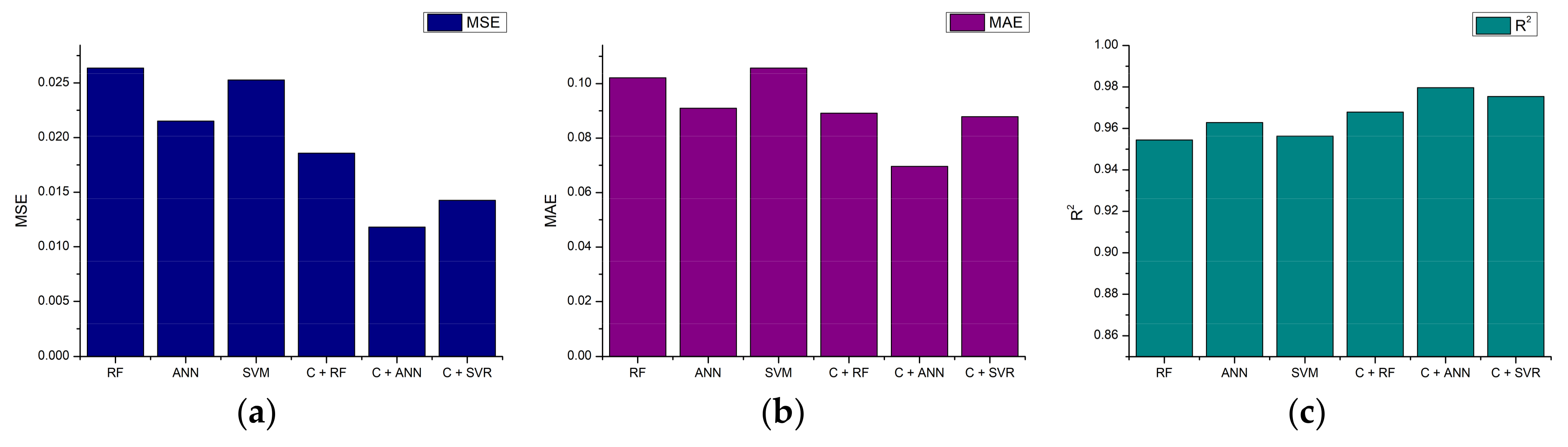
5.3.2. Output Power Estimation

The same types of regressors as those described in the wave tank experiment were used to predict the output power in the onsite experiment. The experimental results show that the regressor combined with a classifier exhibited better performance than one without a classifier in this experiment, as well. However, the performance difference among the three machine learning algorithms in Figure 11 is smaller than that of the wave tank experiment in Figure 9. It is also noticeable that the MSE and MAE in Figure 11 are less than those in Figure 9 because the output power was measured in watts (W) in Figure 9, while kilo-watts (kW) in Figure 11. Therefore, the prediction error is higher for Figure 11. From both experiments, we can confirm that the proposed regressors are efficient and accurate regardless of the algorithms used in predicting the output power from the movement of the buoys.

6. Conclusions

Renewable energy is considered as an option to reduce the use of natural resources and to mitigate climate change. Despite high power density and low environmental impact, wave energy has not been as widely explored as solar and wind. A number of devices and mechanisms has been proposed to harvest wave energy, but the development of effective and efficient energy converting methods remains a challenge.
In this study, we proposed an approach to predict the output power of a nearshore wave energy converter (WEC) based on the movement of the floating buoy and using machine learning algorithms. Since the output power from wave energy harvesting stations varies greatly with the location of installation and other non-human factors, it is important to design an effective prediction model to find optimal locations. The WEC device used in this study is comprised of an energy absorbing unit and a power generating unit. To monitor the movement of the buoy, we developed a data collection module that incorporates a microcontroller, a gyro-accelerometer sensor and a wireless transceiver. The data for the experiments were collected from a wave tank simulator and an actual wave energy harvesting plant. We thoroughly analyzed the collected dataset by applying several machine learning techniques. We proposed models for prediction based on SVM, RF and ANN. Experimental results indicated that the combined model, which is a classifier followed by regressor, worked accurately enough to be utilized to predict the output power from the movement of a buoy. The developed model is useful for finding the optimal locations for wave harvesting plants and to guide the design of the buoy to maximize output power.

Acknowledgments

This work was supported by the 2016 research fund of Myongji University.

Author Contributions

Henock Mamo Deberneh carried out the experiments. Henock Mamo Deberneh and Intaek Kim wrote the paper under the supervision of Intaek Kim. Intaek Kim finalized the paper.

Conflicts of Interest

The authors declare no conflict of interest.

References

  1. Drew, B.; Plummer, A.R.; Sahinkaya, M.N. A review of wave energy converter technology. Proc. IMechE Part A 2009, 223, 887–902. [Google Scholar] [CrossRef]
  2. Cruz, J. Ocean Wave Energy: Current Status and Future Prespectives; Springer: Berlin/Heidelberg, Germany, 2007. [Google Scholar]
  3. Brekken, T.K.; Von Jouanne, A.; Han, H.Y. Ocean wave energy overview and research at oregon state university. In Proceedings of the Power Electronics and Machines in Wind Applications, Lincoln, NE, USA, 24–26 June 2009; Volume 24, pp. 1–7. [Google Scholar]
  4. Kim, G.; Jeong, W.M.; Lee, K.S.; Jun, K.; Lee, M.E. Offshore and nearshore wave energy assessment around the korean peninsula. Energy 2011, 36, 1460–1469. [Google Scholar] [CrossRef]
  5. Korea Energy Agency. Available online: http://www.energy.or.kr/renew_eng/new/standards.aspx (accessed on 2 February 2018).
  6. Sung, Y.; Kim, J.; Lee, D. Power Converting Apparatus. U.S. Patent 20150275847A1, 1 October 2015. [Google Scholar]
  7. Margheritini, L.; Vicinanza, D.; Frigaard, P. Ssg wave energy converter: Design, reliability and hydraulic performance of an innovative overtopping device. Renew. Energy 2009, 34, 1371–1380. [Google Scholar] [CrossRef]
  8. Czech, B.; Bauer, P. Wave energy converter concepts: Design challenges and classification. IEEE Ind. Electron. Mag. 2012, 6, 4–16. [Google Scholar] [CrossRef]
  9. Jang, H.S.; Bae, K.Y.; Park, H.-S.; Sung, D.K. Solar power prediction based on satellite images and support vector machine. IEEE Trans. Sustain. Energy 2016, 7, 1255–1263. [Google Scholar] [CrossRef]
  10. Phaiboon, S.; Tanukitwattana, K. Fuzzy model for predicting electric generation from sea wave energy in Thailand. In Proceedings of the Region 10 Conference (TENCON), Singapore, 22–25 November 2016; pp. 2646–2649. [Google Scholar]
  11. Shi, J.; Lee, W.-J.; Liu, Y.; Yang, Y.; Wang, P. Forecasting power output of photovoltaic systems based on weather classification and support vector machines. IEEE Trans. Ind. Appl. 2012, 48, 1064–1069. [Google Scholar] [CrossRef]
  12. Perera, K.S.; Aung, Z.; Woon, W.L. Machine learning techniques for supporting renewable energy generation and integration: A survey. In Proceedings of the International Workshop on Data Analytics for Renewable Energy Integration, Nancy, France, 19 September 2014; Springer: Cham, Switzerland, 2014; pp. 81–96. [Google Scholar]
  13. Ingine, Inc. Available online: http://www.ingine.co.kr/en/ (accessed on 2 February 2018).
  14. Deberneh, H.M.; Kim, I. Wave Power Prediction Based on Regression Models. In Proceedings of the 18th International Symposium on Advanced Intelligent Systems, Daegu, Korea, 11–14 October 2017. [Google Scholar]
  15. Banos, O.; Galvez, J.-M.; Damas, M.; Pomares, H.; Rojas, I. Window size impact in human activity recognition. Sensors 2014, 14, 6474–6499. [Google Scholar] [CrossRef] [PubMed]
  16. Hira, Z.M.; Gillies, D.F. A review of feature selection and feature extraction methods applied on microarray data. Adv. Bioinform. 2015, 2015. [Google Scholar] [CrossRef] [PubMed]
  17. Juszczak, P.; Tax, D.; Duin, R.P. Feature scaling in support vector data description. In Proceedings of the ASCI; Citeseer: State College, PA, USA, 2002; pp. 95–102. [Google Scholar]
  18. Wold, S.; Esbensen, K.; Geladi, P. Principal component analysis. Chemom. Intell. Lab. Syst. 1987, 2, 37–52. [Google Scholar] [CrossRef]
  19. Samuel, A.L. Some studies in machine learning using the game of checkers. IBM J. Res. Dev. 1959, 3, 210–229. [Google Scholar] [CrossRef]
  20. Chapelle, O.; Vapnik, V.; Bousquet, O.; Mukherjee, S. Choosing multiple parameters for support vector machines. Mach. Learn. 2002, 46, 131–159. [Google Scholar] [CrossRef]
  21. Liaw, A.; Wiener, M. Classification and regression by randomforest. R News 2002, 2, 18–22. [Google Scholar]
  22. Peres, D.; Iuppa, C.; Cavallaro, L.; Cancelliere, A.; Foti, E. Significant wave height record extension by neural networks and reanalysis wind data. Ocean Model. 2015, 94, 128–140. [Google Scholar] [CrossRef]
  23. Raschka, S. Python Machine Learning; Packt Publishing Ltd.: Birmingham, UK, 2015. [Google Scholar]
  24. Hsu, C.-W.; Chang, C.-C.; Lin, C.-J. A Practical Guide to Support Vector Classification; National Taiwan University: Taipei City, Taiwan, 2003. [Google Scholar]
  25. Scikit Learn. Available online: http://scikit-learn.org/stable/modules/generated/sklearn.svm.SVC.html (accessed on 2 February 2018).
  26. Trivedi, S.; Pardos, Z.A.; Heffernan, N.T. Clustering students to generate an ensemble to improve standard test score predictions. In Proceedings of the International Conference on Artificial Intelligence in Education, Auckland, New Zealand, 28 June–1 July 2011; Springer: Berlin/Heidelberg, Germany, 2011; pp. 377–384. [Google Scholar]
Figure 1. Schematic diagram of nearshore WEC configuration [13].
Applsci 08 00566 g001
Figure 2. Working principle of the nearshore WEC [13] (a) when the buoy rises and (b) when the buoy descends.
Applsci 08 00566 g002
Figure 3. Schematic diagram of the data collection procedure.
Applsci 08 00566 g003
Figure 4. Data collection module (left: transmitter; right: receiver).
Applsci 08 00566 g004
Figure 5. Schematic diagram of the proposed system.
Applsci 08 00566 g005
Figure 6. Scene from the wave tank experimental site.
Applsci 08 00566 g006
Figure 7. INGINE wave energy harvesting station. (a) Scene from the experimental site located at Bukchon in Jejudo. (b) Simulated arrangement of the connecting ropes of the buoy.
Applsci 08 00566 g007
Figure 8. Performance evaluation on different window sizes for prediction.
Applsci 08 00566 g008
Figure 9. Comparison of predictors based on: (a) MSE; (b) MAE; (c) R2.
Applsci 08 00566 g009
Figure 10. Performance evaluation on different window sizes for prediction.
Applsci 08 00566 g010
Figure 11. Comparison of predictors based on: (a) MSE; (b) MAE; (c) R2.
Applsci 08 00566 g011
Table 1. Three cases for the experiment.
Experimental CasesActual ValuesScaled ValuesScaled Average Power (W)
HeightPeriodHeightPeriod
Case 14 m12 s20 cm2.68 s9.36
Case 23 m10 s15 cm2.24 s5.82
Case 32.5 m10 s12.5 cm2.24 s3.22
Table 2. Evaluation metrics (ns: number of samples).
MetricDefinition
MAE = 1 n s i = 0 n s 1 | y ^ i y i |
MSE = 1 n s i = 0 n s 1 ( y ^ i y i ) 2
R 2 = 1 i = 0 n s 1 ( y ^ i y i ) 2 i = 0 n s 1 ( y i y ¯ ) 2
Table 3. Window size vs. the numbers of training and testing datasets.
Window Size12182426323672
Number of training657438329303246220111
Number of testing2821891421311069548
Table 4. Training and testing sample sizes of the experiments.
Window Size600120018002400300036004200480054006000
Number of training362518131208906725604518453403362
Number of testing1554777519389311260222195173156

