Article

Acceleration Harmonic Estimation for Hydraulic Servo Shaking Table by Using Simulated Annealing Algorithm

College of Mechanical and Electrical Engineering, Harbin Engineering University, Harbin 150001, China
*
Author to whom correspondence should be addressed.
Appl. Sci. 2018, 8(4), 524; https://doi.org/10.3390/app8040524
Submission received: 15 March 2018 / Revised: 22 March 2018 / Accepted: 28 March 2018 / Published: 29 March 2018
(This article belongs to the Section Mechanical Engineering)

Abstract

:
In order to study the anti-shock performance of equipment under different working conditions, a hydraulic servo shaking table is used to replicate the desired motion with high fidelity. However, the sinusoidal acceleration response waveform is not a pure sinusoid due to the inherent nonlinearities within the system. The generating higher harmonic deteriorates the control performance and leads to system instability. To suppress the harmonic distortion and accurately estimate harmonic information, the harmonic estimation scheme based on simulated annealing algorithm is proposed. The sum of error square between actual value and estimated value is defined as the objective function. The amplitude and phase of each harmonic can be directly extracted when the objective function is minimized. Simulation and experimental results indicate that the proposed algorithm has good convergence performance and high estimation precision.

1. Introduction

A shaking table is usually used to replicate various vibration conditions that occur in civil engineering, automation industry, and aseismatic performance tests [1,2,3,4,5]. According to the drive mode, a shaking table falls into categories of mechanical shaking tables, electrical shaking tables, and hydraulic servo shaking tables. Hydraulic servo shaking tables are widely used in the engineering field because of their advantages: higher force-to-weight ratio, higher response speed, higher load stiffness, and control precision [6]. However, they have many drawbacks, such as a dead zone in the servo valve, friction and backlash in joints, and the dynamic characteristic in hydraulic actuator [7]. Due to the above nonlinear factor, the sinusoid acceleration response shows amplitude attenuation and phase delay, which causes waveform distortion. The harmonic distortion deteriorates the control performance of system and leads to system instability [8]. In order to suppress harmonic distortion and precisely reproduce the desired signal, it is necessary to obtain the amplitude and phase of the each harmonic component. Furthermore, the estimated information can be used to compensate for the harmonic distortion [9].
In past decades, various estimation methods have been developed in order to accurately estimate harmonic information. The most widely used method is the fast Fourier transform (FFT). Nevertheless, this method has some problems, namely aliasing, leakage, and picket-fence effect, which could result in harmonic estimation inaccuracy [10]. Some recursive algorithms, like the least mean square (LMS) and recursive least square (RLS), are also proposed to solve harmonic estimation problem [11,12,13]. Ray et al. developed the ensemble Kalman filter to estimate the amplitude and phase of distorted power system signal [14,15]. Barros presented the wavelet-packet transform to estimate the harmonic groups in voltage and current waveforms [16]. Sahoo et al. studied a digital algorithm for harmonic identification based on complex H∞ filter [17]. Soliman et al. utilized a new algorithm based on fuzzy linear regression to estimate the frequency and harmonic component of the voltage signal in a power network [18]. With the development of intelligent optimization theory, it offers the possibility of estimating the harmonic component with modern optimal algorithm [19]. Almaita and Asumadu applied the radial basis function (RBF) neural network to duly estimate harmonic components of converter waveforms [20]. Wang used a Hopfield neural network to simultaneously determine the supply frequency variation, the amplitude variation and phase variation of fundamentals, as well as each harmonic [21]. Ray et al. proposed particle swarm optimization (PSO) algorithm to identify current harmonic associated with fundamental current from measurement [22]. Ji et al. adopted an adaptive bacterial swarming (ABS) algorithm to dynamically estimate the frequencies and phases of the voltage or current harmonics in power grids [23].
The difficulty in harmonic estimation is due to the fact that harmonic generating is dynamic and nonlinear in nature. Thus, fast and accurate harmonic estimation approaches are required. However, the aforementioned methods can only be implemented offline and have several limitations on convergence and accuracy. In this paper, the simulated annealing optimization algorithm is used for hydraulic servo shaking table acceleration harmonic estimation. Simulation and experimental results indicated that the proposed algorithm can accurately estimate the amplitude and phase of each harmonic. Furthermore, the estimation algorithm has better real time performance and convergence performance when compared with conventional algorithm, such as RLS.

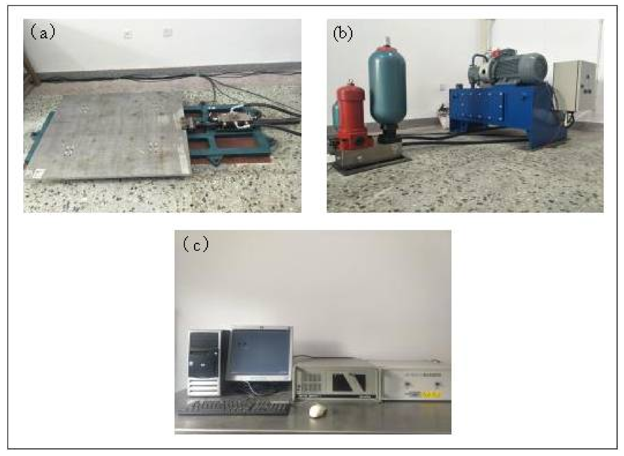
2. Hydraulic Servo Shaking Table
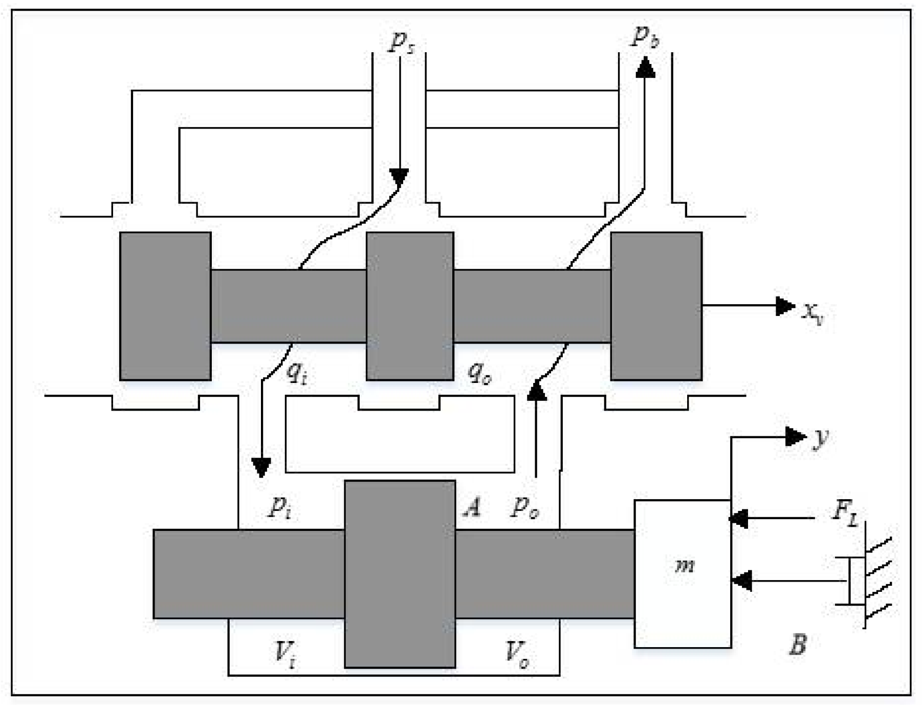
Figure 1 shows the hydraulic servo shaking table developed by Harbin Engineering University, which includes three subsystems: mechanical system, hydraulic system, and control system. The mechanical system consist of a platform and a symmetric cylinder controlled by a two-stage symmetric servo valve. The hydraulic system is used to provide hydraulic energy and control the pressure and flows of servo actuator. The control system consists of a host computer and a target computer. The host computer serves as user interface and allows users to generate a command signal, and obtain current experiment data. The real time control algorithm and serial communication with the programmable logic controller are operated on the target computer. Some main parameters of the shaking table are listed in Table 1.

2.1. Dynamic Model

The power mechanism of the hydraulic servo shaking table includes servo valve, hydraulic cylinder, and load, which can be simplified as symmetric hydraulic cylinder controlled by four-way valve. The schematic diagram of the power mechanism is shown in Figure 2, where p s and p b are the supply/return pressure, q i and q o are the input/output oil flow of the cylinder, p i and p o are the input/output pressure, V i and V o are the input/output oil volume, m is the mass, x v is the valve position, B is the piston’s viscous damping coefficient, y is the load position, A is the effective area of the cylinder. The physical features of shaking table’s hydraulic system can be described by the following three equations.
The linearized flow equation of the servo valve can be expressed as
q L = K q x v K c p L
where q L = ( q i + q o ) / 2 is load flow, K q = q L / x v is flow gain, p L = p i p o is pressure burden, K c = q L / p L is flow-pressure coefficient.
The flow continuity equation of the cylinder is
q L = A d y d t + C t p p L + V t 4 β e · d p L d t
where C t p is leakage coefficient, V t = V i + V o is the total volume of the actuator’s two chambers, β e is the effective bulk modulus.
The force balance equation is
F g = A ( p i p o ) = A p L = m d 2 y d t 2 + B d y d t + F L
Performing Laplace transform from Equation (1) to Equation (3), the transfer function G p ( s ) from the valve displacement x v to the hydraulic cylinder displacement y can be expressed as
G p ( s ) = Y X v = K q / A s ( s 2 ω h 2 + 2 ζ h ω h s + 1 )
where ω h = 4 β e A 2 m V t is load inherent resonant frequency, ζ h = K c A β e m V t + B c 4 A V t β e m is load damping ratio.

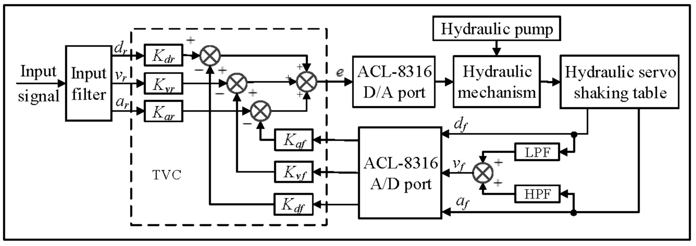
2.2. Control Principle

Figure 3 shows the schematic diagram of the hydraulic servo shaking table. The three variable controller (TVC) is a commonly used controller for shaking table [24]. The three variable of TVC represent displacement, velocity, and acceleration of the shaking table. The TVC feedforward gain ( K d r , K v r , K a r ) is used to improve system stability and the feedback gain ( K d f , K v f , K a f ) is used to extend frequency bandwidth and reduce tracking error. The velocity feedback signal is usually synthesized from the measured displacement and acceleration, as it is difficult to measure the displacement, velocity, and acceleration simultaneously. The velocity in the high/low frequency range is obtained from the displacement/acceleration using a high pass filter (HPF) or low pass filter (LPF), respectively. The measured displacement, velocity, and acceleration are acquired by the ACL-8316 A/D port, transforming analogue signal into digital signal. The input signal is obtained by input filter. The TVC compares the feedback signal ( d f , v f , a f ) with the given signal ( d r , v r , a r ) to generate the control signal e, which is sent to hydraulic actuator by means of ACL-8316 D/A port that transforms digital signal into analogue signal. Hydraulic power is supplied by the hydraulic pump to drive the hydraulic cylinder, causing the desired movement of hydraulic servo shaking table.

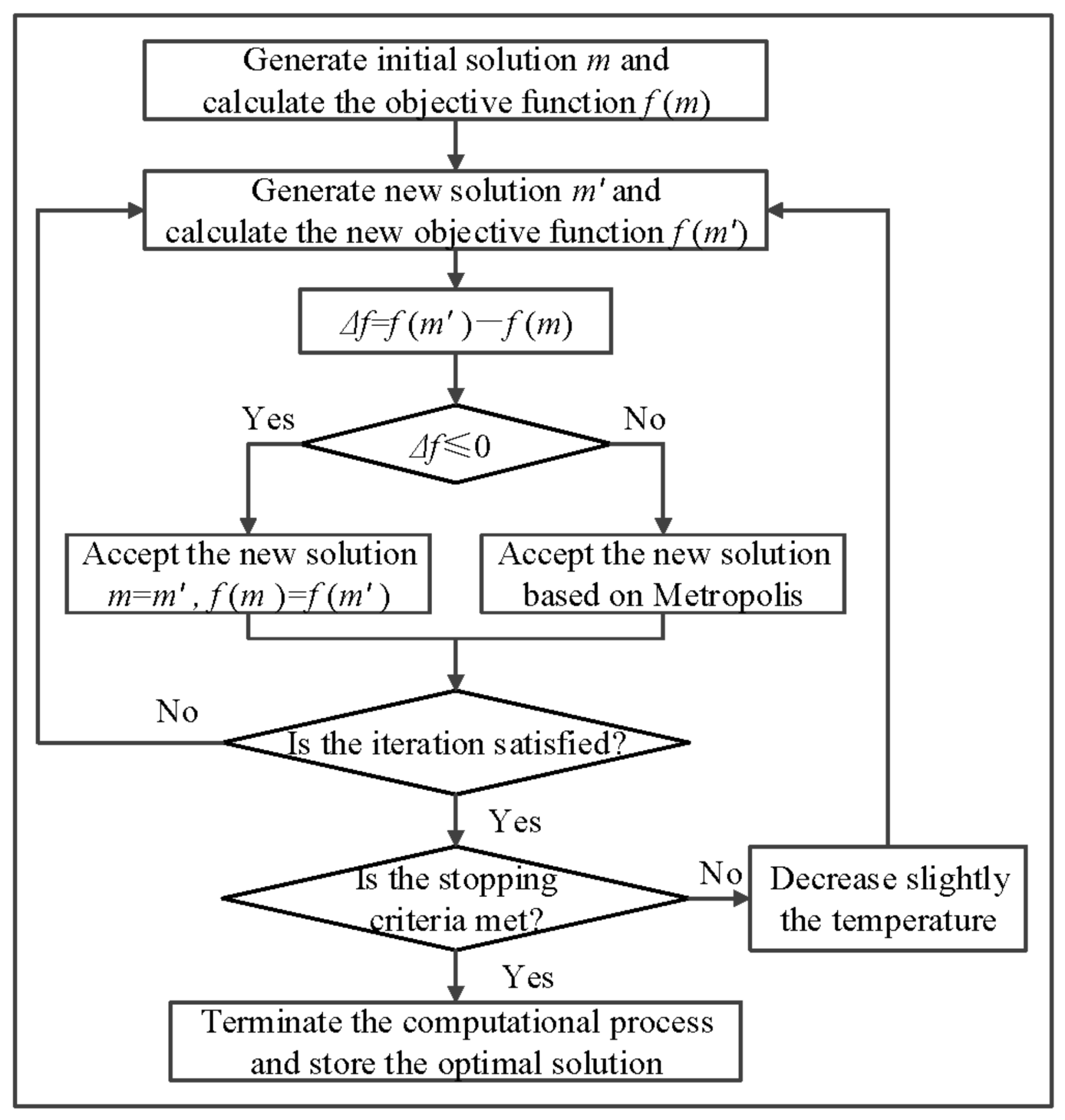
3. Simulated Annealing Algorithm

The simulated annealing is a population based stochastic algorithm, which was first introduced by Metropolis in 1953 [25]. Since then, it has been widely used to solve combination optimization problem. The algorithm stimulates the process of heating up a solid to a high temperature followed by slow cooling [26,27,28,29,30,31]. As the temperature goes up, the particles of solid change into disordered state, causing an increase in internal energy. However, the internal energy of solid decreases with a drop in temperature, and the particles gradually back in order. If the cooling rate is cooled slowly enough for the solid, the particles can reach thermal equilibrium at each temperature [32]. The minimum energy is obtained by reaching the ground state of room temperature. According to the Metropolis guidelines, the probability of particles tend to become equilibrium state exp ( Δ f / k T ) at a given temperature T, where k denotes the Boltzmann constant. Assuming a solid in current state m0 with energy level f(m) and the next state m′ with energy level f(m′), if the difference between the two energy levels is less than or equal to zero, the new state m is accepted. Otherwise, if the difference Δ f = f ( m ) f ( m ) is greater than zero, the new state is accepted with Metropolis criteria. The acceptance probability is compared to a number P r [ 0 , 1 ] generated randomly and m is accepted whenever P > P r . The initial temperature T0 is supposed to be high enough to allow acceptance of any new state in the first step. In each step, the procedure generates a fixed number of neighborhood solutions and evaluates them using the current temperature value T s = α T 0 , where α ( 0 < α < 1 ) is an attenuation factor [33,34]. The proposed simulated annealing algorithm used in this paper can be summarized as Figure 4.

4. Harmonic Estimation Scheme

The distorted signal can be considered as the sum of fundamental response and harmonic component. Each harmonic has its own amplitude and phase, and a frequency that is integral multiple of the fundamental response. Therefore, the sinusoidal acceleration response of the shaking table at time t can be expressed by
a ( t ) = n = 1 N A n sin ( n ω t + ϕ n )
where N represents the order of the harmonic; ω is the fundamental frequency; An and φn are the amplitude and phase of nth harmonic, respectively.
The discrete time version of Equation (5) can be represented as
a ( k ) = n = 1 N A n sin ( n ω k + ϕ n )
For estimating amplitude and phase, Equation (6) can be rewritten as
a ( k ) = n = 1 N ( A n cos ϕ n sin n ω k + A n sin ϕ n cos n ω k )
Define x n 1 = A n cos ϕ n , x n 2 = A n sin ϕ n . Then, Equation (7) can be written as
a ( k ) = n = 1 N ( x n 1 sin n ω k + x n 2 cos n ω k )
Sinusoidal signal in parametric form becomes
a ( k ) = h ( k ) x ( k )
where h ( k ) = [ sin ω k ,   cos ω k ,   sin 2 ω k ,   cos 2 ω k ,     , sin N ω k ,   cos N ω k ] T is the input vector and x ( k ) = [ x 11 ,   x 12 ,   x 21 ,   x 22 ,     x N 1 ,   x N 2 ] T is the weight vector.
The estimation model for the algorithm is
a ^ ( k ) = h ( k ) x ^ ( k )
where x ^ ( k ) is the estimation weight vector.
The estimate value x ^ ( k ) for the requested parameters x ^ ( k ) can be obtained by minimizing the objective function
f ( x ) = n = 1 N [ e ( k ) ] 2 = n = 1 N [ a ( k ) a ^ ( k ) ] 2
The harmonic estimation scheme based on simulated annealing algorithm can be illustrated with Figure 5. The sinusoidal acceleration response is used as desired signal, and the reference harmonic generates the input vector. The error between the actual value and the estimated value is optimized using simulated annealing algorithm. The problem is formulated as an optimization problem, where the goal is to minimize the objective function. After updating the weight vector, the amplitude and phase of the fundamental and nth harmonic are derived as follows
{ A n = x n 1 2 + x n 2 2 ϕ n = tan ( x n 2 / x n 1 )
Moreover, fundamental as well as each harmonic can be directly extracted from the final updated weights
a ^ n ( k ) = x n 1 sin n ω k + x n 2 cos n ω k

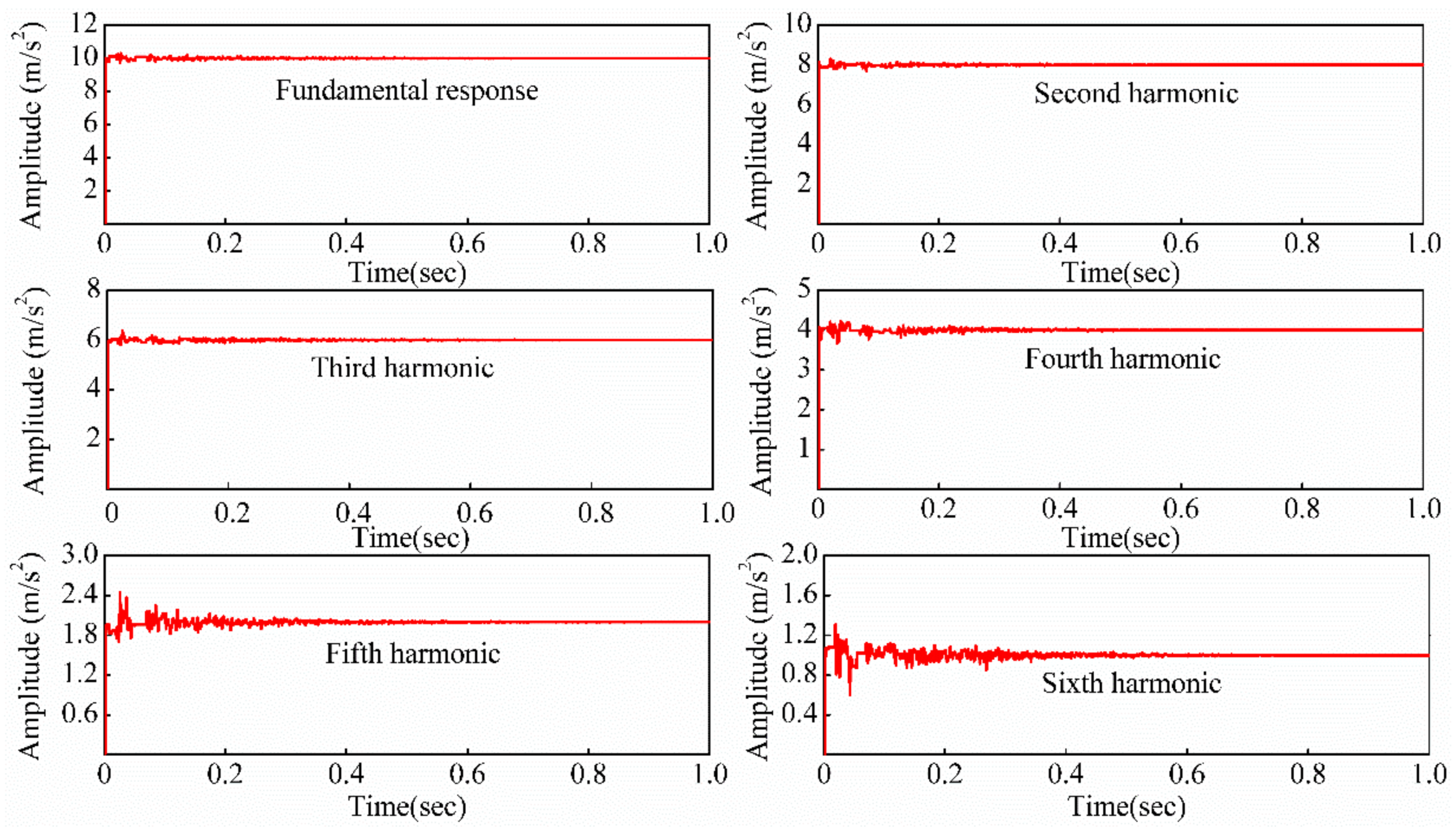
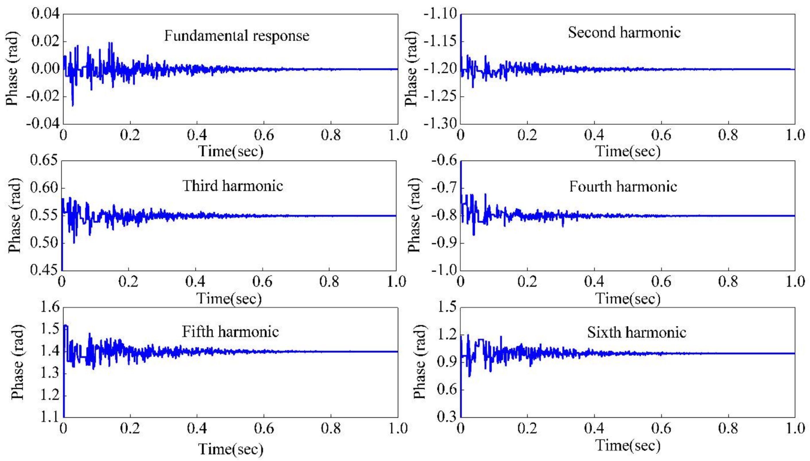
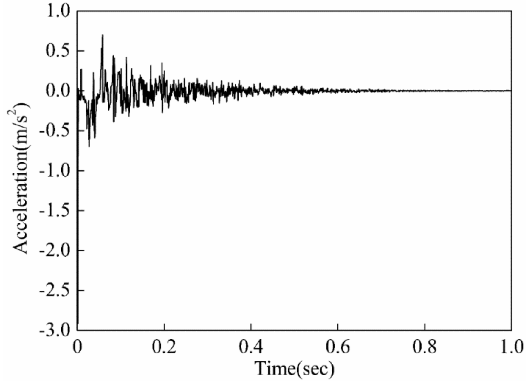
5. Simulation and Results

In order to verify the effectiveness of the developed acceleration harmonic estimation algorithm, the simulation is firstly implemented. The simulation signal contains six harmonic. It is
a ( t ) = 10 sin ( 10 π t ) + 8 sin ( 20 π t 1.2 ) + 6 sin ( 30 π t + 0.55 ) + 4 sin ( 40 π t 0.8 ) + 2 sin ( 50 π t + 1.4 ) + 1 sin ( 60 π t + 1 )
Figure 6 and Figure 7 are the estimated amplitudes and phases, respectively. It is seen that the estimated values converge to their corresponding original values after about 0.4 s. Figure 8 shows the error between the given signal a ( t ) and the estimated signal a ^ ( t ) along with time. The estimation error is asymptotically converged to zero within 0.4 s, which means that the given signal is estimated precisely. The amplitude and phase of each estimated harmonic when they in stable states are listed in Table 2 with its given value. At the same time, it is clear that the estimated amplitude and phases are very close to its given value for each harmonic. Thus the developed acceleration harmonic estimation scheme can estimate harmonic information efficiently.

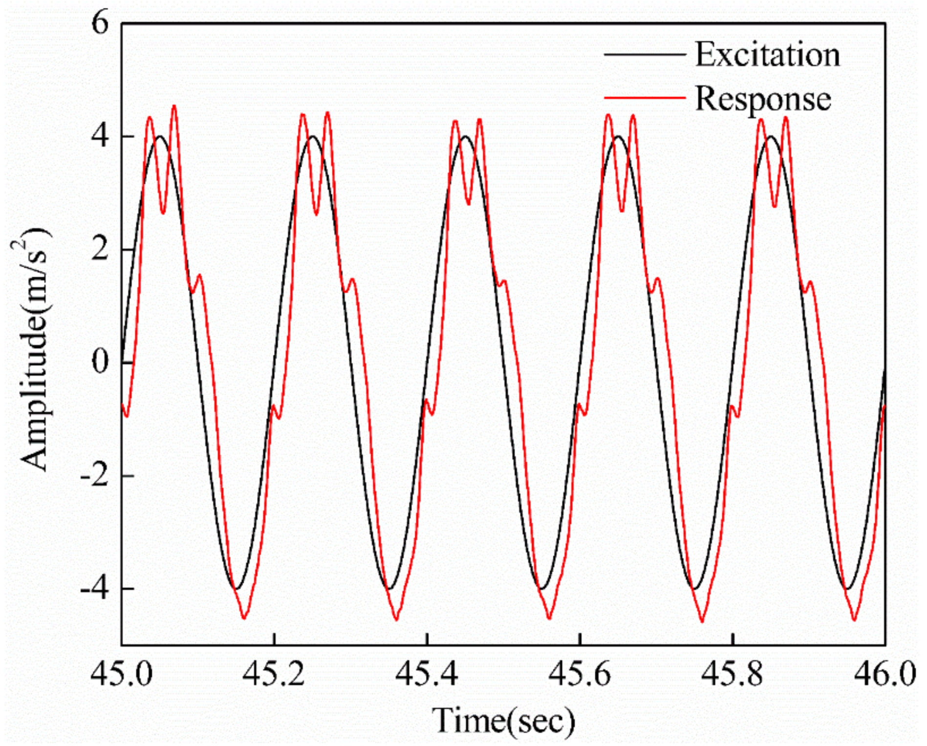
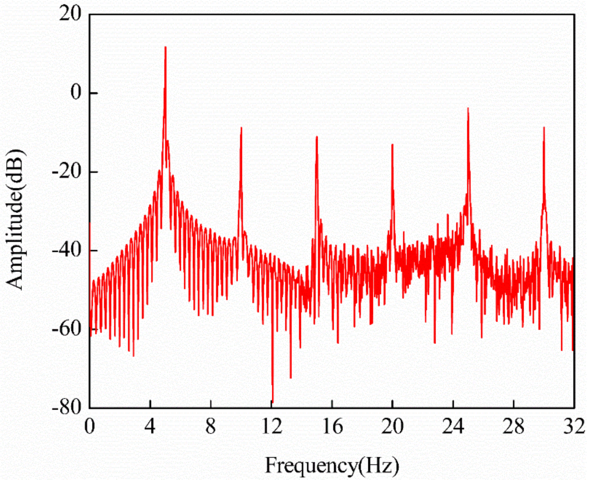
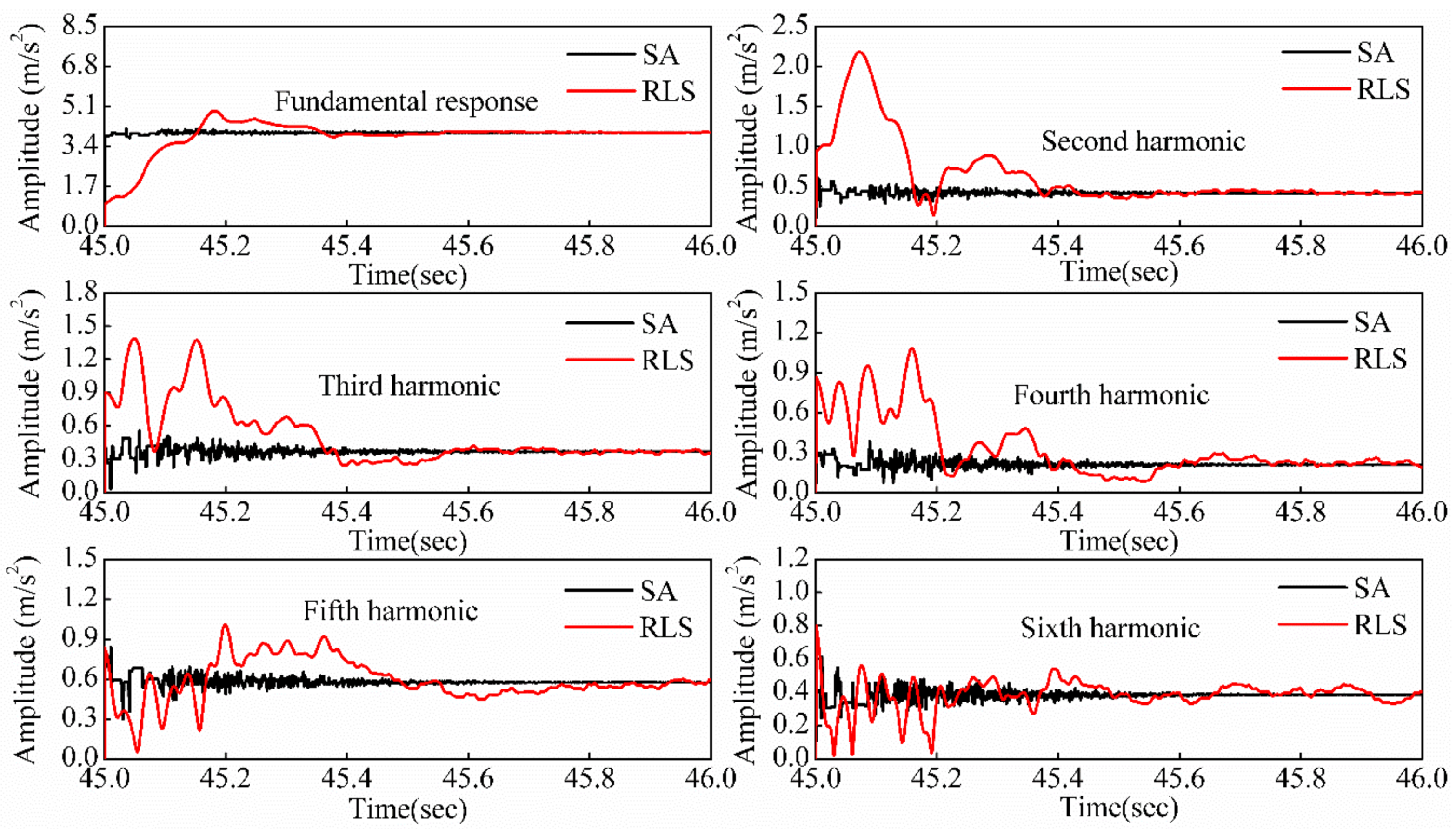
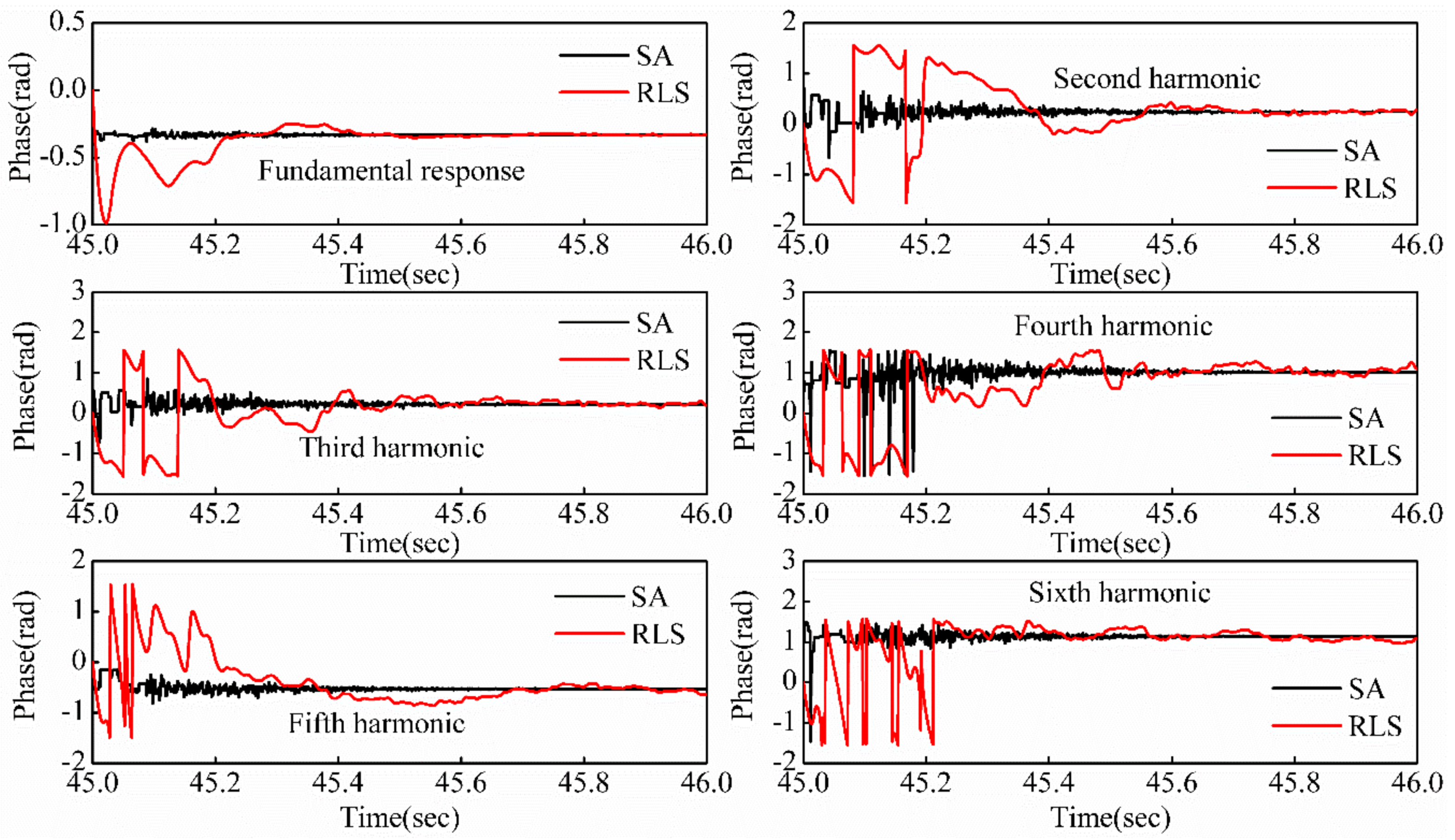
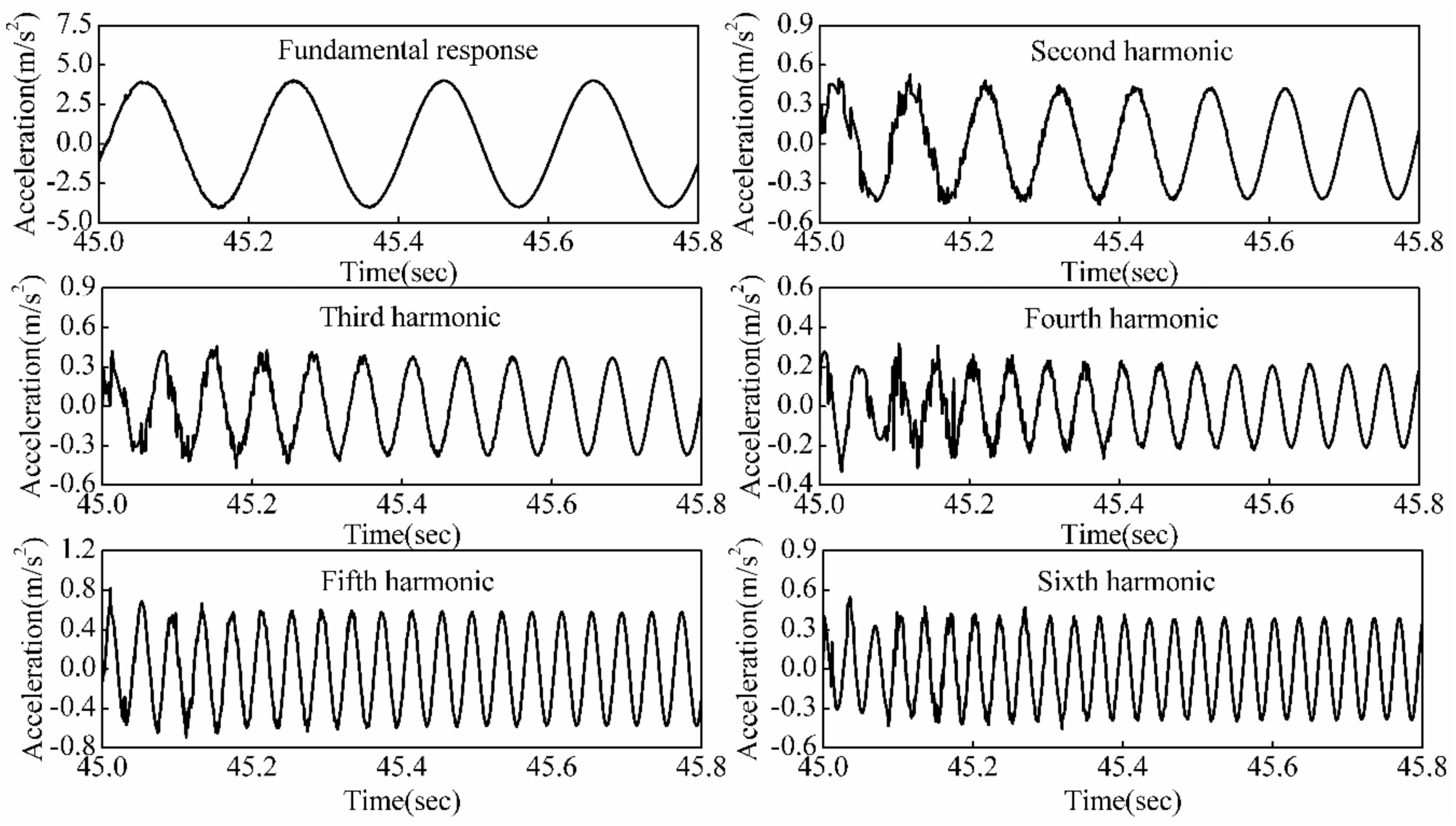
6. Experiment and Results

When the acceleration excitation is 4 sin ( 2 π × 5 t )   m / s 2 , the excitation signal and acceleration response in the time domain are shown in Figure 9. It can be seen that the acceleration response is seriously distorted, due to the effects of nonlinearities in the hydraulic servo shaking table. Since higher harmonics are less dominant in all harmonics, the harmonic estimation is usually up to sixth harmonic in practical applications. The amplitude frequency diagram computed by FFT in Figure 10 indicates that the fundamental response is at 5 Hz, the second harmonic is at 10 Hz, the third harmonic is at 15 Hz, and so on. The total harmonic distortion (THD) is a very important criterion to evaluate its waveform performance and it is given by
THD = A 2 2 + A 3 2 +     A N 2 A 1 × 100 %
where A1 is the amplitude of the fundamental, A2 the amplitude of the second harmonic, A3 the amplitude of the third harmonic, and so on.
The result of THD based on FFT is calculated off line as shown in Table 3. It can be seen that the fifth harmonic plays a vital role in all harmonics, and the fourth harmonic is the least harmonic. The THD is 22.22%, which is a large value.
Figure 11 and Figure 12 represent the amplitude and phase estimation results respectively using simulated annealing and RLS algorithm of the given acceleration response. As can be seen from the figures, RLS based estimation method has large estimation error and oscillatory in the initial stage of estimation process, though it converges to the stable value. From the perspective of harmonic estimation, the estimated algorithm by simulated annealing is better than RLS in real time performance and convergence performance. In addition, each harmonic can be directly extracted from the distortion signal. Its results are shown in Figure 13, from which it can be seen that there are large fluctuations at the beginning of the estimation, but converge quickly to its steady states within 0.5 s.

7. Conclusions

Due to the inherent nonlinearities within the hydraulic servo shaking table, the acceleration response produced is a time varying signal. Thus, fast and accurate harmonic estimation algorithm is required. In this paper, the simulated annealing optimization algorithm is performed on the acceleration sinusoidal response replication. Simulation and experimental results show that the harmonic estimation scheme can estimate the amplitude and phase of each harmonic and reconstruct individual harmonics at the same time. As an intelligent optimization technique, the proposed algorithm does not require a priori knowledge of the system.
Compared with conventional RLS algorithms, experimental results show that the proposed simulated annealing algorithm is better in convergence performance and real time performance. This is important for harmonic estimation and harmonic suppression. In addition, the proposed technique can be extended to many areas: online estimation, optimization, and control problems.

Acknowledgments

This project is supported by National Natural Science Foundation of China (grant no. 51375102), the Fundamental Research Funds for the Central Universities (grant no. HEUCFP201733).

Author Contributions

Jianjun Yao and Zhenshuai Wan conceived the flow chart of simulated annealing algorithm. Zhenshuai Wan wrote the main manuscript and develop the mathematical modeling of power mechanism and control scheme. Jianjun Yao, Zhenshuai Wan, and Yu Fu analyzed the results and refine the submitted manuscript.

Conflicts of Interest

The authors declare no conflict of interest.

References

  1. Shen, G.; Lv, G.M.; Ye, Z.M.; Cong, D.C. Implementation of electrohydraulic shaking table controllers with a combined adaptive inverse control and minimal control synthesis algorithm. IET Control Theory Appl. 2011, 5, 1471–1483. [Google Scholar] [CrossRef]
  2. Xu, Y.; Hua, H.; Han, J. Modeling and controller design of a shaking table in an active structural control system. Mech.Syst. Signal Process. 2008, 22, 1917–1923. [Google Scholar] [CrossRef]
  3. Tang, B.; Li, X.; Chen, S.; Xiong, L. Shaking Table Test of a RC Frame with EPSC Latticed Concrete Infill Wall. Shock Vib. 2017, 2017, 1–18. [Google Scholar] [CrossRef]
  4. Li, W.; Liu, W.; Wang, S.; Du, D. In-Plane Strengthening Effect of Prefabricated Concrete Walls on Masonry Structures: Shaking Table Test. Shock Vib. 2017, 2017, 1–13. [Google Scholar] [CrossRef]
  5. Zhang, L.; Cong, D.; Yang, Z.; Zhang, Y.; Han, J. Optimal Design and Hybrid Control for the Electro-Hydraulic Dual-Shaking Table System. Appl. Sci. 2016, 6, 220. [Google Scholar] [CrossRef]
  6. Shen, W.; Wang, J.Z.; Wang, S.K. The control of the electro-hydraulic shaking table based on dynamic surface adaptive robust control. Trans. Inst. Meas. Control 2016, 39, 1271–1290. [Google Scholar] [CrossRef]
  7. Yao, J. Acceleration Harmonic Cancellation of Electro-hydraulic Servo Shaking Table. J. Mech. Eng. 2010, 46, 22–28. [Google Scholar] [CrossRef]
  8. Yao, J.; Xiao, R.; Chen, S.; Di, D.; Gao, S.; Yu, H. Acceleration harmonic identification algorithm based on the unscented Kalman filter for shaking signals of an electro-hydraulic servo shaking table. J. Vib. Control 2014, 21, 3205–3217. [Google Scholar] [CrossRef]
  9. Tanaka, T.; Nishida, Y.; Funabiki, S. A method of compensating harmonic currents generated by consumer electronic equipment using the correlation function. IEEE Trans. Power Deliv. 2004, 19, 266–271. [Google Scholar] [CrossRef]
  10. Freijedo, F.D.; Doval-Gandoy, J.; Lopez, O.; Penalver, C.M. Novel Harmonic Identification Algorithm Based on Fourier Correlation and Moving Average Filtering. In Proceedings of the Power Engineering Society General Meeting, Tampa, FL, USA, 24–28 June 2007; pp. 1–6. [Google Scholar]
  11. Singh, G.K. Power system harmonics research: A survey. Int. Trans. Electr. Energy Syst. 2009, 19, 151–172. [Google Scholar] [CrossRef]
  12. Lin, H.C. Power Harmonics and Interharmonics Measurement Using Recursive Group-Harmonic Power Minimizing Algorithm. Eng. Lett. 2011, 2191, 1184–1193. [Google Scholar] [CrossRef]
  13. Bettayeb, M.; Qidwai, U. Recursive estimation of power system harmonics. Electr. Power Syst. Res. 1998, 47, 143–152. [Google Scholar] [CrossRef]
  14. Ray, P.K.; Subudhi, B. Ensemble-Kalman-Filter-Based Power System Harmonic Estimation. IEEE Trans. Instrum. Meas. 2012, 61, 3216–3224. [Google Scholar] [CrossRef]
  15. Gomez-Acedo, E.; Olarra, A.; Orive, J.; de la Calle, L.N.L. Methodology for the design of a thermal distortion compensation for large machine tools based in state-space representation with Kalman filter. Int. J. Mach. Tools Manuf. 2013, 75, 100–108. [Google Scholar] [CrossRef]
  16. Barros, J.; Diego, R.I. Application of the wavelet-packet transform to the estimation of harmonic groups in current and voltage waveforms. IEEE Trans. Power Deliv. 2006, 21, 533–535. [Google Scholar] [CrossRef]
  17. Sahoo, H.K.; Dash, P.K.; Rath, N.P. Frequency estimation of distorted non-stationary signals using complex H ∞ filter. AEUE Int. J. Electron. Commun. 2012, 66, 267–274. [Google Scholar] [CrossRef]
  18. Soliman, S.A.; Alammari, R.A.; El-Hawary, M.E. Frequency and harmonics evaluation in power networks using fuzzy regression technique. Electr. Power Syst. Res. 2003, 66, 171–177. [Google Scholar] [CrossRef]
  19. Du, K.L.; Swamy, M.N.S. Search and Optimization by Metaheuristics: Techniques and Algorithms Inspired by Nature; Springer: Basel, Switzerland, 2016. [Google Scholar]
  20. Kumar, N.S.; Shrinivasarao, B.R.; Pai, P.S. Radial Basis Function Neural Network (RBFNN) Based Modeling in Liquified Petroleum Gas (LPG)-Diesel Dual Fuel Engine with Exhaust Gas Recirculation (EGR). Ind. J. Sci. Technol. 2016, 9. [Google Scholar] [CrossRef]
  21. Wang, P.; Zou, Y.; Zou, S.; Sun, Y. Hopfield Neural Network-based Estimation of Harmonic Currents in Power Systems. In Proceedings of the WCICA 2006 the Sixth World Congress on Intelligent Control and Automation, Dalian, China, 21–23 June 2006; pp. 7494–7497. [Google Scholar]
  22. Ray, P.K.; Subudhi, B. BFO optimized RLS algorithm for power system harmonics estimation. Appl. Soft Comput. 2012, 12, 1965–1977. [Google Scholar] [CrossRef]
  23. Ji, T.Y.; Li, M.S.; Wu, Q.H.; Jiang, L. Optimal estimation of harmonics in a dynamic environment using an adaptive bacterial swarming algorithm. IET Gen. Trans. Distrib. 2011, 5, 609–620. [Google Scholar] [CrossRef]
  24. Tagawa, Y.; Kajiwara, K. Controller development for the E-Defense shaking table. Proc. Inst. Mech. Eng. Part I J. Syst. Control Eng. 2007, 221, 171–181. [Google Scholar] [CrossRef]
  25. Li, S.; Chen, Y.; Du, H.; Feldman, M.W. A genetic algorithm with local search strategy for improved detection of community structure. Complexity 2010, 15, 53–60. [Google Scholar] [CrossRef]
  26. El-Naggar, K.M.; Alrashidi, M.R.; Alhajri, M.F.; Al-Othman, A.K. Simulated Annealing algorithm for photovoltaic parameters identification. Sol. Energy 2012, 86, 266–274. [Google Scholar] [CrossRef]
  27. Rajan, C.C.A.; Mohan, M.R. An evolutionary programming based simulated annealing method for solving the unit commitment problem. Power Syst. IEEE Trans. 2007, 19, 577–585. [Google Scholar] [CrossRef]
  28. Green, P.L. Bayesian system identification of a nonlinear dynamical system using a novel variant of Simulated Annealing. Mech. Syst. Signal Process. 2015, 52–53, 133–146. [Google Scholar] [CrossRef]
  29. Palacios, J.A.; Olvera, D.; Urbikain, G.; Elías-Zúñiga, A.; Martínez-Romero, O.; Lacalle, L.N.L.; Rodríguez, C.; Martínez-Alfaro, H. Combination of simulated annealing and pseudo spectral methods for the optimum removal rate in turning operations of nickel-based alloys. Adv. Eng. Softw. 2018, 115, 391–397. [Google Scholar] [CrossRef]
  30. Sechen, C. Placement and Global Routing of Integrated Circuits Using the Simulated Annealing Algorithm. Ph.D. Dissertation, University of California, Berkeley, CA, USA, 1986. [Google Scholar]
  31. Lutfiyya, H.; Mcmillin, B.; Poshyanonda, P.; Dagli, C. Composite stock cutting through simulated annealing. Math. Comput. Model. Int. J. 1992, 16, 57–74. [Google Scholar] [CrossRef]
  32. Rajan, C.C.A. Hydro-thermal unit commitment problem using simulated annealing embedded evolutionary programming approach. Int. J. Electr. Power Energy Syst. 2011, 33, 939–946. [Google Scholar] [CrossRef]
  33. Bouleimen, K.; Lecocq, H. A new efficient simulated annealing algorithm for the resource-constrained project scheduling problem and its multiple mode version. Eur. J. Oper. Res. 2003, 149, 268–281. [Google Scholar] [CrossRef]
  34. Olvera, D.; Elías-Zúñiga, A.; Martínez-Alfaro, H.; Lacalle, L.N.L.; Rodríguez, C.A.; Campa, F.J. Determination of the stability lobes in milling operations based on homotopy and simulated annealing techniques. Mechatronics 2014, 24, 177–185. [Google Scholar] [CrossRef]
Figure 1. The hydraulic servo shaking table. (a) Mechanical system; (b) hydraulic system; (c) control system.
Applsci 08 00524 g001
Figure 2. Schematic diagram of the hydraulic system.
Applsci 08 00524 g002
Figure 3. Control principal of the hydraulic servo shaking table.
Applsci 08 00524 g003
Figure 4. Flow chart of the simulated annealing algorithm.
Applsci 08 00524 g004
Figure 5. Block diagram of the harmonic estimation scheme.
Applsci 08 00524 g005
Figure 6. Estimation of amplitude.
Applsci 08 00524 g006
Figure 7. Estimation of phase.
Applsci 08 00524 g007
Figure 8. Estimation of error.
Applsci 08 00524 g008
Figure 9. The response in time domain.
Applsci 08 00524 g009
Figure 10. The response in frequency domain.
Applsci 08 00524 g010
Figure 11. Estimation of amplitude.
Applsci 08 00524 g011
Figure 12. Estimation of phase.
Applsci 08 00524 g012
Figure 13. Estimation of each harmonic.
Applsci 08 00524 g013
Table 1. The main parameters of shaking table.
ComponentParameter
Piston diameter40 mm
Rod diameter35 mm
Stroke25 mm
Supply pressure8 Mpa
Frequency range0~50 Hz
Maximum velocity1.4 m/s
Maximum acceleration10 m/s2
Table 2. The estimated value compared with given value.
Harmonic OrderGiven ValueEstimated Value
Amplitude (m/s2)Phase (rad)Amplitude (m/s2)Phase (rad)
Fundamental response1009.999816−0.000004
Second harmonic8−1.28.000417−1.19999
Third harmonic60.555.9998530.550035
Fourth harmonic4−0.84.000689−0.79981
Fifth harmonic21.41.9992841.399997
Sixth harmonic110.9997760.999728
Table 3. Total harmonic distortion analysis result.
THDHarmonic Amplitude (m/s2)
22.22%A1A2A3A4A5A6
3.98300.41620.35100.19710.58240.3306

