Abstract
In order to lower the dependence on textual annotations for image searches, the content based image retrieval (CBIR) has become a popular topic in computer vision. A wide range of CBIR applications consider classification techniques, such as artificial neural networks (ANN), support vector machines (SVM), etc. to understand the query image content to retrieve relevant output. However, in multi-class search environments, the retrieval results are far from optimal due to overlapping semantics amongst subjects of various classes. The classification through multiple classifiers generate better results, but as the number of negative examples increases due to highly correlated semantic classes, classification bias occurs towards the negative class, hence, the combination of the classifiers become even more unstable particularly in one-against-all classification scenarios. In order to resolve this issue, a genetic algorithm (GA) based classifier comity learning (GCCL) method is presented in this paper to generate stable classifiers by combining ANN with SVMs through asymmetric and symmetric bagging. The proposed approach resolves the classification disagreement amongst different classifiers and also resolves the class imbalance problem in CBIR. Once the stable classifiers are generated, the query image is presented to the trained model to understand the underlying semantic content of the query image for association with the precise semantic class. Afterwards, the feature similarity is computed within the obtained class to generate the semantic response of the system. The experiments reveal that the proposed method outperforms various state-of-the-art methods and significantly improves the image retrieval performance.
1. Introduction
With the advent of digital cameras and multimedia applications, image libraries over the Internet have seen dramatic expansion. To explore these libraries, as well as access to the appropriate information without a text-based description of every image, has motivated research in the domain of content based image retrieval (CBIR). Automatically retrieving images have also found vast applications in many other fields, including architectural design [1], geographical information systems [2], surveillance systems [3], remote sensing [2], etc. [4,5,6].
CBIR systems consider visual attributes of images, such as colour, shape, texture and salient image points, to build feature repository. Closely resembled images, in terms of the feature distance, are returned as the semantic response of a CBIR system against queries acquired in the form of images. However, due to the inherent gap between high level semantics prevailing in images and low level feature representations, the image retrieval performance of CBIR systems is poor. In order to enhance image retrieval performance, many researchers [7,8,9] have used machine learning algorithms to understand image semantics through feature representations and gained remarkable results [10]. Aschraf et al. applied multi-class support vector machines (SVM) on the feature repository obtained by the Bandlet transform [8]. Xue et al. achieved the structural granularity through the combination of structured large margin machine (SLMM) and the Laplacian-SVM (LapSVM) for image retrieval [11]. Tan et al. applied a graph based clustering method to obtain a semantic association of image queries [12]. Sen Wang et al. applied a multi-tasking support machine for optimal feature selection and image retrieval [13].
No matter how image classification occurs, classifier learning becomes a real challenge when training sets are severely imbalanced (i.e., the class of interest is under represented in the training set) particularly in the presence of overlapping semantic classes with a small sample size [14]. The evaluation criterion that guides the learning procedure leads to ignoring minority class examples, and resultantly the induced classifier loses its classification ability. As a usual example, consider a bi-class dataset with imbalance ratio of 1:100; a classifier that tries to maximize the accuracy of classification may end up with an accuracy of 90% by only discounting the positive examples. The chances of incorrect association further increase when the training set comprises of multiple highly correlated classes, as is the case in CBIR.
In order to overcome the class imbalance problem for CBIR, in our previous work [15] we introduced the concept of positive sample generation through genetic algorithm (GA) and used it with SVMs. The basic idea behind the work was simple, that the samples of a class of interest can be grown through the existing class examples through genetic operations. However, the major drawback of the technique was that the objective function of the GA ignores the optimal samples if their similarity index exceeds a threshold based on the search space. Another limitation of the technique was that there was no concept of the elite offspring that also result in the form of weak features. The method also needs a specific set of features and was not generic. Due to these loopholes, the performance of the algorithm degrades significantly when the number of classes increase or the feature extraction mechanism changes. Therefore, to overcome these limitations, and to effectively address the problem of CBIR, a concept of Genetic classifier comity learning (GCCL) is introduced in this paper. The proposed GCCL scheme combines multiple SVM and artificial neural networks (ANN) classifiers through GA-based asymmetric and symmetric bagging and resolves the class imbalance problem, and hence results in the form of stable classification. The reason to introduce GA-based asymmetric and symmetric bagging is that the simple combination of classifiers impacts negatively over each other in the presence of under represented classes and becomes unstable and results in the form of low accuracy. Contrary to our previous approach [15], which defines the objective function of GA at the population level and ignores the individual chromosomes, in the present work, the objective function of GA compares multiple chromosome populations and generates strong features by extending the chromosomes that pass the defined evaluation test.
2. Related Work
The class imbalance problem is one of the many challenges that the machine learning community is facing [14,16]. This imposes a critical situation to address, as many real world classification problems (including CBIR) are seriously suffering from it. To improve the classification results, several research works are accounting this issue.
Qi et al. proposed a cross-category label propagation algorithm to enhance image retrieval performance in the presence of small sample sets [17]. The algorithm can directly propagate the inter-category knowledge at the instance level between source and target categories. Furthermore, the algorithm can automatically detect conditions under which the transfer process may become detrimental to the learning process, so it can avoid the propagation of the knowledge from those categories.
Yang et al. presented a null space locality preserving the discriminant analysis method for facial recognition [18]. The method projected the training samples into a scatter matrix that are then randomly sampled through bagging to generate a set of bootstrap replicas. The overall goal of the technique was to improve the face recognition performance by alleviating the over-fitting due to large null spaces.
Zhang et al. presented a conformal kernel transformation for SVM to address the class imbalance problem [19]. For this an approximated hyperplane of the SVM was obtained and a kernel function was applied by computing the parameters through the chi-square test. Maratea et al. improved the association capability of SVM by surpassing the approximate solution through kernel transformation [20]. The asymmetric space around the class boundary was enlarged that compensates the data skewness in binary classification. Tao et al. addressed the issue of imbalanced sets by generating multiple versions of SVM classifier by replacing negative samples with the positive duplicates [21]. Improvement in the image retrieval occurs with this approach but it is not significant when feedbacks are severely imbalanced. The similar approach was followed in [22] with expectation maximization (EM) for parameter estimation in relevance feedback (RF)-based CBIR. Chang et al. modified the kernel matrix of the SVM to address the bi-class imbalance problem [23].
In [24], performance refinements of AdaBoost were exhibited on imbalanced datasets. As a first step, the dataset was over-sampled and the standard AdaBoost was applied. In the next step, the parameters of classifiers were obtained through GA. The sampling and re-weighing strategy tuned the AdaBoost towards a given performance measure of interest by not exceeding the computational overhead. Belattar et al. performed feature selection through GA and linear discriminant analysis (LDA) for dermatological image retrieval [25]. The algorithm evolves the feature vectors through the binary-GA and performs feature selection through LDA that are then classified through the k-nearest neighbors (KNN) classifier. Luong et al. proposed a GA-based simultaneous classifier for image annotation and region label assignment [26]. The algorithm represents various image regions through feature vectors and selects the salient features through GA that are then used to train the multi-classifier ensembles for image annotation. Irtaza et al. used GA for increasing the relevant output for semantic webs [27]. The system considers the user search preferences and applies GA to improve the output after multiple feedback rounds.
Most of the described techniques were designed for dealing with the class imbalance problem that spans only to the two-class scenarios. However, the application of bi-class resolutions usually appear to be less effective or even cause a negative impact when implied in the multi-class situations [28].
3. Class Imbalance Problem
In classification, a multi class dataset D can be described as: where with is the particular class with similar instances and the class of interest is imbalanced when . The situation becomes more challenging when classes are highly correlated, i.e., in image classification. Due to the high correlation, the miss-association rate is high as it increases the classification bias towards the negative class, i.e., due to the fewer instances in . The diversity of the content in the training samples also favours the incorrect associations.
Class imbalance also raises a series of issues that further increase the difficulty of learning, namely, small sample size, overlapping or class separability, and small disjuncts. The presence of small disjuncts in a dataset occurs when the concept represented by the minority class is formed of sub-concepts. Besides, small disjuncts are implicit in most of the problems. The existence of sub-concepts also increases the complexity of the problem because the amount of instances among them is not usually balanced [14].
3.1. Dealing with Class Imbalance
As the imbalanced dataset is a critical issue in data classification, therefore, a lot of techniques have been developed to effectively address this problem. These techniques can broadly be classified into three groups [14]:
- Algorithm level approaches: These approaches adapt the existing classifier to bias their learning towards the minority class. The knowledge about the application domain and the corresponding classifier is required by these methods to comprehend the reasons for classifier failure in the presence of uneven class distribution.
- Data level approaches: These approaches proceed by re-balancing the class distribution by re-sampling the data space. Due to their versatility, these methods can be applied with any classifier. The class imbalance effect is decreased with a data preprocessing step.
- Cost-sensitive learning: These frameworks add the misclassification cost to the instances and bias the classifier towards the class having the higher misclassification costs that is usually the minority class. The overall goal is to minimize the total cost errors of both classes. However, as the misclassification costs are not explicitly available in the datasets, these techniques cannot be tuned in a practical manner.
- Ensemble Approaches: The ensemble based techniques that combine multiple classifiers for classification are appearing as another category to address the class imbalance problem [29]. The ensemble based methods are usually applied in combination with any of the approaches mentioned earlier.
In the current work we have applied the data pre-processing approach with GCCL based ensembles to generate a new hybrid method to address the class imbalance problem for image classification in CBIR. In the present work, the class imbalance problem in image classification is considered as an optimization problem and our target is to maximize the relevant results against the image queries.
3.2. Classifier Ensembles
Combining classifiers is a developed research area in pattern recognition to develop highly accurate and reliable systems. In most of the pattern recognition applications, a single algorithm cannot uniquely represent the problem in an optimal way. Moreover, the generalization attributes of each classification algorithm are very sensitive to the model and parameter selection steps. Instead of keeping only one classification algorithm, if we combine several classification algorithms, we can bring more reliability [30] and accuracy [31] in the results [32].
While approaching towards an efficient classifier ensemble, it is necessary that the complexity of testing process should not increase in a way that isn’t appropriate for a real time application. So this could be achieved through one of the following ensemble design strategies [32]:
- Combine different classifiers or learning algorithms instead of keeping only one classifier which is giving the lowest estimation value of the expected risk.
- For a given learning algorithm, apply various initialization procedures or model selection strategies to obtain different candidate solutions. After obtaining candidate solutions, combine them.
- Generate subsets of training set or feature sets and train several classifiers on these subsets. Some classifiers can be more efficient on local subspaces and they will act like experts on their local domain.
Breiman [33] introduced the concept of bagging that is also known as Bootstrapped Aggregation. Bagging combined voting with a vote generation process to obtain multiple classifiers. The idea behind bagging is to allow each base classifier to be trained on different random subsets of training examples, so that the base classifiers can become more diverse [34]. Bringing diversity in classifiers is a historically accepted area of research in the domain of ensemble learning, that increases the classification performance.
It is commonly admitted that a large diversity amongst the classifiers in a team is preferred. However, depending on the context, diversity can be understood differently. For example one can view it as complementarity, or even orthogonality, between classifiers, or it can be considered as a measure of dependence [33]. Diversity is often used implicitly in the ensemble growing techniques, where the ensembles become progressively diverse. Another use of diversity is its application as optimization criterion for ensemble training. Finally, diversity controls the ensemble pertinence by checking if it is diverse enough [32]. An example of diversity method is bagging that generates several diverse base classifiers. The bagging makes use of original training set to generate multiple bootstrap training sets from it, so that a classifier can be generated to become a part of the ensemble.
From a training set having N training examples, a bootstrap training set can be generated by performing N multinomial trials in such a way that one example is drawn out from the training set in each trial. In each trial every example present in the training set has a probability 1/N of being drawn out. Bootstrap sampling does exactly this N times, and selects a number r in the range of 1 to N. The algorithm selects the r-th training example and add it to the bootstrap training set S.Which means that, some examples will be chosen more then one time to become the part of training set, while there will be some examples present in the original training set, that will never be able to become the part of bootstrapped training set. In bagging, several classifiers are generated by creating M such bootstrap training sets. The bagging algorithm returns a function which is used to classify new examples on the basis of voting through the base models . The corresponding class y is considered as one which gets the maximum number of votes.
In general, bagged ensembles work better if the learning models are unstable. This can also be stated as: the bagging does more to reduce the variance in the base models than the bias. Therefore, bagging performs best, relative to its base models, when the base models have high variance and low bias [34].
3.3. Motivations of Genetic Algorithm for Class Imbalance
The distance between two feature vectors can be minimized by simple perturbation. Keeping this analogy in mind, GA is used to extend the sample set by generating a uniform feature vector set for skewed category of images. Details of the process are presented in this section. As elaborated in Figure 1, these feature vectors serve as the representation of the virtual images in the skewed category that have the image portions from multiple samples already present in the skewed class and that are generated by the GA at the time of feature extraction. The proposed GA based architecture effectively handles the classifier bias problem and ensures better image retrieval output.
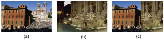
Figure 1.
Virtual image generation through genetic algorithm (GA). (a) and (b) are original images; (c) is the virtual image generated by combining image regions.
Proof of Effectiveness
Consider the case of regression in which training data can be represented as: , where are the observations in the form of feature vectors, are the corresponding outputs, and are number of training examples. For training data, our goal is to generate the optimal parameters that may reduce the difference between the known output and the computed output based on the feature observations. The cost function can be represented as:
where
and are corresponding features in the feature vector x. The optimal selection of parameters ensures minimum value of the cost function in Equation (1). The parameters can be optimized through the gradient decent algorithm for every j as:
where is learning rate and it’s value is predefined. The probabilistic interpretation of the phenomena is given by:
Now consider the case of normal CBIR approach where our target is to obtain the top k most similar images against a query image in terms of distance, i.e., the images that give the minimum distance in terms of features. Therefore, the objective function of CBIR can be expressed as:
Here is the query image and are the images present in the image repository in the form of feature vectors, whereas, represents the objective function of CBIR that targets the k most similar images against a query image that have lowest aggregate distance. The probabilistic interpretation of Equation (5) can be given as:
Equation (6) shows that the semantic output is normally distributed and objective function of Equation (5) is very similar to Equation (1) but parameter that exists in Equation (2) does not exists in Equation (5). Therefore, there is no way to optimize the usual output that appears on the base of features and depends on the robustness of features; in case of weak features the semantic output cannot be improved. Here it is important to mention that as the parameter in Equation (1) can be optimized through various algorithms, for example, gradient decent, conjugate gradient, etc., and therefore even the weak features lead to the right output. However, as in Equation (5), there is no way by which we can optimize features, therefore, output of CBIR system may remain inappropriate. In order to overcome this drawback, we have found a new feature similarity measure that allows us to explore the feature space through the perturbation of features, and based on this we extend the objective function of CBIR as:
Equation (7) describes that we generate different representations of feature vectors and to obtain feature similarities and select a set of the k most similar images as system response. The probabilistic interpretation of the Equation (7) can be given as:
From Equation (8) we can observe that the parameter of Equation (1) is compromised with the parameter in Equation (7), and, even with the week features the semantic response of the system, improves which clearly signifies the effectiveness of the approach. Equation (7) is further extended in subsequent sections to resolve the class imbalance problem.
3.4. Genetic Algorithm Architecture for Class Imbalance Problem
In order to resolve the class imbalance problem through GA, the approach we followed is to extend the feature-base of the skewed class with more positive examples. For this, GA considers feature vectors in the skewed class to generate feature representations of the virtual images (Figure 1) by applying genetic operators. The details of the process will appear in subsequent sections. As feature vectors contain global features, therefore the virtual image representations (chromosome offspring) are even more powerful as they contain global feature components of multiple images. To further ensure that GA receives good features in every generation, we evaluate the chromosome population through the objective function that defines multiple chromosome populations and we select the most optimal one—to achieve this goal, we have modified the objective function that we defined in Equation (7). The GA in the present work is designed by keeping the single objective in mind that classifier ensembles generate precise semantic output by not suffering from imbalanced training samples.
3.4.1. Feature Extraction and Chromosome Generation
For image representation in the form of feature vectors, we analyzed images through Curvelet transform, Wavelet packets and Gabor filters. In this section, we briefly cover the feature extraction process, but for detailed information please refer our previous work [15]. However, the proposed GA architecture is independent of the mentioned features and can be applied with any other type of feature extraction method.
- Curvelet Transform: The Curvelet transform was originally proposed to overcome the missing directional selectivity of conventional 2D discrete wavelet transforms (DWTs). The 2D Curvelet transform allows an almost optimal sparse representation of objects with singularities along smooth curves [35].As a first step of feature extraction, we represent images in the Curvelet transform via wrapping and obtain multiple bands and sub-bands. For every sub-band, we compute the variance of image transformation, and for every band, we take the mean of the variances of the associated sub-bands. These mean values are placed in a vector, which serves as the Curvelet representation.
- Wavelet Packets: As a second step of feature extraction, the complete wavelet packets tree [36] of image is computed with 64 nodes. From this tree we select more predictable nodes on the basis of Shanon entropy and compute the standard deviation as the feature of the corresponding node. These standard deviation values are placed in a vector that serves as the feature representation of the wavelet packets tree.
- Gabor Filters: We take the smallest approximation image of wavelet packets tree for Gabor analysis. The convolution kernels are defined as:whereis the standard deviation of the Gaussian function, is the wavelength of the harmonic function, is the orientation, and is the spatial aspect ratio, which is left constant at 0.5. For obtaining the Gabor responses, images are convolved by the kernels of size 9 × 9. In our implementation 12 kernels are used, which are tuned to four orientations () and three frequencies (). Orientation, varies from 0 to (stepping by ) and frequency varies from 0.3 to 0.5. After generating the response images following scheme is used for feature extraction:Twelve Gabor based response images are obtained by applying the above mentioned parameters. Corresponding to every response image, we obtain the eigenvalues in the form of vectors. Each vector is represented by a single value that is obtained by taking the mean. Therefore, finally there will be twelve mean values as the final representation by the Gabor transform.
Final image representations are obtained by collecting the features of the Curvelet transform, Wavelet packets, and Gabor filters in a single vector that serves as the feature vector of corresponding image. These feature vectors are used as the chromosomes in the GA to overcome the class imbalance problem for the skewed class. In the current proposal, the Chromosomes are defined as:
where N are the number of genes in one chromosome represented by , and M is the population size. The initial population of chromosomes consists of the original feature vectors present in the skewed class, and serves as the parent chromosomes that reproduce through the genetic operators.
3.4.2. Genetic Operators
According to Algorithm 1, we generate a population of the chromosomes (feature vectors) through the genetic operators, namely, crossover and mutation. As we want to hold the good balance between the exploration and exploitation, the population size is kept constant, that is equal to , and the crossover and mutation are applied as the genetic operators for generating new offspring. The technique we are using for offspring generation works by slightly modifying the two-point discrete crossover operator (DCO) [37]. The basic theme of the two-point DCO is to randomly select the two crossover points, and exchange the segments of the parents to generate two offspring. The value of each gene (single feature in a feature vector in our case) in the offspring coincides with the value of one of the parents [37]. In our work, the offspring are generated by exchanging the segments of the parents by following a range based approach. For offspring generation, two parents with corresponding gene cut-point positions are randomly selected as:
where and are two randomly selected chromosomes, and and are two cut-point positions, respectively. Whereas, generates random numbers between 1 to M to randomly select two parents from the population of M chromosomes present in the skewed class. Similarly, generates random numbers between 1 to N to randomly select cut-point positions for first and second parent. The newly generated offspring can be defined as:
For offspring generation, genes of both parents are merged according to the Equations (15) and (16). If the random number reveals the same parent, i.e., , then the mutation operator is applied through the gene flip method that generates a perturbation in the cut-point ranges and generates a single offspring as:
In the current implementation, the mutation rate is 0.05 as the higher mutation rates turn the search into a primitive random search [38].
| Algorithm 1 Genetic Algorithm. |
| Input: Positive set , number of generated populations , population size ‘P’, GA method ‘m’. |
|
3.4.3. Fitness Function and Termination Conditions
In order to resolve the class imbalance problem we grow the skewed class with more positive examples. The fitness function is employed to determine the optimal solutions that could enhance the image classification results when classified through the GCCL based classifier ensembles. For fitness evaluation we have used the following function:
According to the fitness function , we are comparing the chromosome populations with the actual training examples present in the skewed class in terms of average distance (where m in Equation (18) represents the total number of samples in the positive class, and 1/2 is just a constant for comprehension) and considering the population of the chromosomes as an optimal set that gives minimum distance. The reason to use the above mentioned fitness function is that we want to generate the chromosome populations that appear similar to the original feature examples. We also evaluate the chromosomes that comprise a population on the basis of chromosome evaluation test and allow or disallow a chromosome to reproduce. The chromosome evaluation test will be discussed in Section 4.1.2.
In our implementation, we generate chromosome populations, and select the optimal set on the basis of the objective function. The termination criterion in our work is the parameter for a particular class . Hence, GA will automatically terminate for a particular class when it selects the optimal population amongst generated populations.
4. Genetic Classifier Comity Learning for Image Classification
The main idea behind this work is that all the images present in the image repository are represented in the form of feature vectors. These feature vectors serve as image signatures to represent the visual attributes of the images. From this feature repository we select a subset of feature vectors from each of the N classes and generate a training repository. As this sub-repository has the representation of the images of the N different classes, therefore samples in each class are naturally skewed compared to the total number of samples of other classes; therefore, before classifier training, we overcome this problem by re-framing the multi-class image classification problem into multiple one class image classification problems. For this, for each class of concern we generate a growing set of positive samples in the class through GA by following an asymmetric and symmetric bagging-based process. The asymmetric and symmetric bagging-based process overcomes the class imbalance problem and provides a working base for the SVM and ANN classifiers. For image classification, we combine the opinions of multiple classifiers through classifier comity learning and as the classification efficiency is strongly dependent upon the training sets that are obtained through the GA, we named the classifier comity learning method as the Genetic classifier comity learning (GCCL) method. Once the classifier training is successfully done, we obtain the semantic association of the query image with respect to the N training classes, and generate the output image-set. Our output image-set comprises of the samples of the obtained semantic class of the query image. For this we compute the distance amongst feature vectors of the query image and feature vectors of the image samples of the obtained semantic class and return the output set comprising images of the closely matched feature vectors. If the output set contains the samples of unwanted classes, then we suppress these samples through relevance feedback. The relevance feedback retrains the model over the user feedbacks in the output set, where images are labelled as either relevant or irrelevant by the system user. Once the retraining is done, the final output is generated, otherwise the user can provide the feedback again. The details of the process are provided in Figure 2 and are discussed in detail in the following subsections.
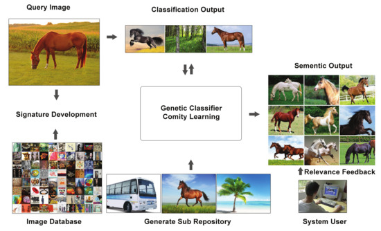
Figure 2.
Architecture of the Proposed Method.
4.1. Image Classification through Support Vector Machines
4.1.1. Asymmetric Bagging Based on Elitism for Support Vector Machines
Bagging incorporates the advantages of bootstrapping and aggregation. Several training sets which are produced by the bootstrapping are used to generate multiple classifiers [21]. In the perspective of binary classification, if we bootstrap the training samples of only one class then bagging is known as asymmetric bagging.
For elitism based asymmetric bagging, we are selecting original chromosomes representing training images present in a skewed class. These chromosomes are used for population generation and newly generated offspring are not allowed to further reproduce. In elitism based asymmetric bagging, positive sample size is equal to the population size, and negative samples are not bootstrapped, therefore all images present in the negative sample set are used for training purposes. The asymmetric bagging procedure is described in Algorithm 2. The Genetic Algorithm (Algorithm 1) considers the case of asymmetric bagging and returns the grown training set on the basis of the objective function. This set is used for the SVM training with the concept of one-against-all (OAA) classification.
| Algorithm 2 Asymmetric bagging based on elite parents through GA for SVM . |
| Input: Positive set , negative set , weak classifier I (SVM), integer (number of generated classifiers) and the test sample x Output: Classifier |
|
4.1.2. Bagging Based on Tournament Selection for Support Vector Machines
For bagging based on tournament selection, newly generated offspring can reproduce as well. However, only those offspring are allowed to reproduce which pass the evaluation test. Our chromosome evaluation test is:
where are the newly generated offspring, are the elite parent chromosomes, and M is the population size. According to the evaluation test we are generating a population of M chromosomes, and allowing only those offspring chromosomes to reproduce that are giving less distance for any of the elite parents. In bagging based on tournament selection, positive and negative sample size is the same in which is equal to the population size. We are randomly selecting samples from the negative set to generate balanced training set. Our bagging procedure is presented in Algorithm 3.
| Algorithm 3 Bagging based on tournament selection through GA for SVM. |
| Input: Positive set , negative set , weak classifier I (SVM), integer (number of generated classifiers) and the test sample x Output: Classifier |
|
4.1.3. Semantic Association Using Support Vector Machines
SVM is known for its amazing accuracy and performance on various pattern recognition problems, and has been acknowledged as a potential and powerful tool for classification problems [22]. For a given training-set having images from N semantic classes, an SVM classifier is defined for a specific class that can be modelled as [39]:
where and are the inputs and corresponding labels, respectively. Samples belonging from the positive class are labelled as and all other samples are labelled as . In feature space, the SVM model takes the form [22]:
where is used as the non-linear mapping to map the input vector into higher dimensional feature space, b is the bias and w is a weight vector of the same dimension as that of the input vector. SVM assumes the linearly separable case as:
However, the image classification in the presence of multiple correlated semantic classes is usually non-linearly separable, therefore, the non-separable case is expressed as:
through the nonlinear kernel function, a maximum margin separating hyperplane can be computed by finding the margin hyperplanes to separate both classes, that transform the problem into a quadratic programming problem as we adopted in the proposed work. In our implementation we used the quadratic kernel which finally results as:
where in Equation (24) is the hyperplane decision function. The Lagrangian multiplier serves as the support vectors and are used to solve the quadratic programming problem that satisfies the Karush Kuhn Tucker (KKT) conditions. The higher values of means the higher prediction confidence, whereas the lower values mean the pattern is close to the boundary. In present work SVM is trained through the asymmetric and symmetric bagging procedures as described earlier.
4.2. Image Classification through Artificial Neural Networks
Asymmetric Bagging for Neural Networks
For all semantic classes, a back-propagation neural network structure is also defined [40] with one hidden layer having 30 neurons and one output unit. For hidden and output layer sigmoid function is used as transfer function. Detail of the neural network structure is summarized in Table 1 and the ANN training procedure is listed in Algorithm 4. One important thing to note is that the neural networks training occurs on the training sets that are obtained by sub-sampling negative class and GA is not involved in this procedure.

Table 1.
Summary of Neural network structure for every image category used in this work.
| Algorithm 4 Asymmetric bagging using neural networks. |
| Input: Positive set , negative set , weak classifier I (ANN), integer (number of generated classifiers) and the test sample x Output: Classifier |
|
4.3. Class Finalization through Genetic Classifier Comity Learning
For GCCL based classification, majority voting rule (MVR) is used in our implementation. MVR does not consider any individual behaviour of the weak classifiers, it only counts the largest number of classifiers that agree with each other [21]. If we have a series of weak classifiers , we can represent MVR as [21]:
For image classification, we combine all the classifiers trained through GA based asymmetric and symmetric bagging procedures resulting in the form of a powerful and stable semantic classifier. Hence, the class of image is one that has a maximum combined association value for SVM and neural network classifiers.
In order to show why our bagging procedure works, consider the following scenario [33]: Let () be a data sample in the training set , where y is the class label of the sample x and L is drawn from a probability distribution P. Suppose is a simple classifier constructed by the asymmetric bagging and symmetric bagging, the aggregated predictor is averaged over L of , i.e., where is the expectation over prediction. If x and y are fixed then
Using and the inequality in Equation (26) in third term,
Integrating both sides of Equation (27) over the sample distribution, the MSE of is smaller than the MSE averaged over L of depending on the inequality of both sides,
The instability effect is clearly visible from the inequality. Two sides will be nearly equal if does not change too much, therefore, in this case, aggregation will not help. If shows high variance then the aggregation will produce more improvement. For stable predictors, this strategy may not work. However, for unstable predictors performance improvement occurs. Neural networks and SVM are unstable for asymmetric bagging and symmetric bagging, therefore strategy improves the retrieval performance.
4.4. Content Based Image Retrieval
Once the classifiers are trained, the semantic association of all the images present in the image repository is determined. The semantic association values are stored in a file that serves as the semantic association database. Therefore, when system suggests the semantic class for any query image, top k images having the same semantic class are returned to the user after ranking on the basis of distance as the image retrieval output.
For some image queries, the system may not be able to determine the right semantic class—the returned output is comprised of the undesired images. To avoid this situation, the system also returns the query top neighbours to the user, and enable relevance feedback over them. Relevance feedback gives freedom to the user to guide the image retrieval system in the case of complex queries to achieve the desired output. Relevance feedback is covered in detail in the experimentation section. Both sets of images are returned to the user in the form of representative images. These representative images are selected from both output sets, and are the images that appear most similar to the query image in terms of distance.
5. Experiment and Results
To evaluate the proposed method, an extensive set of experiments are conducted and performance is evaluated by comparing the proposed algorithm against several state-of-the-art CBIR methods. Details of the experiments and comparative analysis are presented in the following subsections.
5.1. Database Description
To elaborate the effectiveness of the proposed method in terms of content based image retrieval, extensive experiments are conducted on the Corel dataset with 10,908 images. The Corel dataset has two versions, Corel set A and Corel set B. Corel set A has 1000 images grouped in 10 semantic categories namely: Africa, beach, buildings, buses, dinosaurs, elephants, flowers, horses, mountains and food (Figure 3) [41]. Corel set B has 9908 images belonging from several groups like sunset, texture, butterfly, birds, animals, jungle, cars and boats [4]. For implementation of this work, both versions of the Corel datasets are combined, but the results are reported only on the Corel set A, as it is a standard approach followed in several state of the art CBIR systems [4,8,41,42]. Hence, a clear performance comparison is possible. To further elaborate the retrieval performance, the Columbia object image library (COIL) [43] and Caltech-101 [44] datasets are used. The COIL dataset has 7200 images from 100 different semantic groups, whereas the Caltech 101 image set is comprised of 101 different semantic categories.

Figure 3.
Sample images of each category of Corel set A.
5.2. Precision and Recall Evaluation
To evaluate the performance of the proposed method, we determine how many relevant images are obtained in response of image queries. For performance evaluation precision and recall rates are used. Precision determines the ability of system to retrieve only those images that are relevant for image queries in the retrieved output and can be defined as:
Recall rate determines the ability of the classifier system in terms of model association with their actual class [27] and can be defined as:
In our implementation, the results are reported by running a computer simulation for five times that randomly selects twenty image queries from each image category and the precision and recall rates are reported on the top 20 images.
In order to show the superiority of the proposed technique, the results are also compared with those of Dubey et al. [45], Xiao et al. [46], Zhou et al. [47], Shrivastava et al. [48], Kundu et al. [49], Zeng et al. [50], Walia et al. [51], Ashraf et al. [52] and ElAlami et al. [53]. Table 2 presents the class-wise comparison of the proposed system with comparative systems in terms of average precision values. Similarly, Table 3 presents a comparison of the proposed system with comparative systems in terms of average recall values. From the results it can be observed that our proposed system is showing promising precision and recall rates in many categories and has the highest overall precision and recall values against the comparative systems (Table 2 and Table 3).
Table 2.
Comparison of average precision obtained by proposed method and other standard retrieval systems on top 20 retrievals.
Table 3.
Comparison of average recall obtained by proposed method with other standard retrieval systems on top 20 retrievals.
To further elaborate the retrieval capabilities of the proposed method, we have also plotted the precision of the proposed method on different output rates, i.e., from the top 20 to 60 images. For this experiment we run the simulation with same parameter settings as described above, by randomly selecting 200 images (20 images from each image category of Corel A) and running the simulation for five times. The results of the simulation are shown in Figure 4.
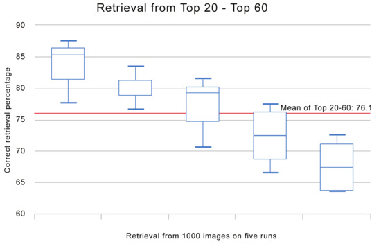
Figure 4.
Image retrieval performance from top 20 to 60 images.
Average precision and recall results from the proposed method over 30 categories of Caltech-101 dataset and over 20 categories from COIL dataset are shown in Figure 5 and Figure 6, respectively.
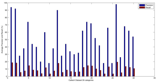
Figure 5.
Average precision and recall results of the proposed method over 30 categories of Caltech-101 dataset.
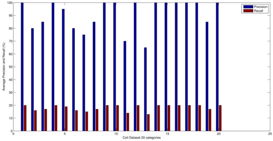
Figure 6.
Average precision and recall results of the proposed method over 20 categories of COIL dataset.
5.3. Bagging Impact
We have also compared the proposed method against the SVM and ANN classifiers to show the performance benefits of GCCL against the individual classifiers. For this the proposed GCCL based system is compared against SVM and ANN classifiers in terms of precision and false positive rates. The reason to use the false positive rates as performance measure is that the lower values of false positive rates are also required for higher classification accuracies.
The results of the comparison are presented in Figure 7 and Figure 8. From the results we can observe that the proposed GCCL based scheme as generates the powerful classifier by overcoming the drawbacks of the weak classifiers hence is much effective and precise in terms of image retrieval.
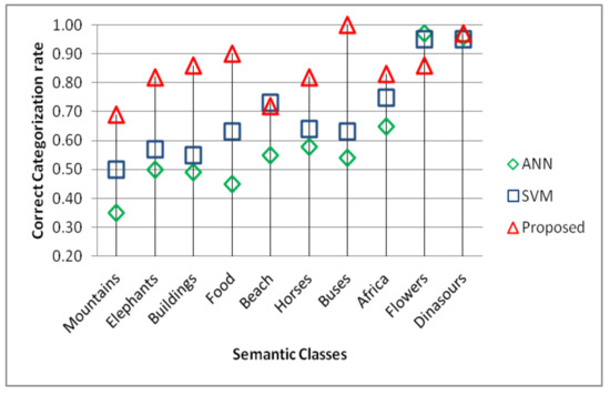
Figure 7.
Image retrieval comparison against artificial neural networks (ANN) and support vector machines (SVM) classifiers in terms of precision.
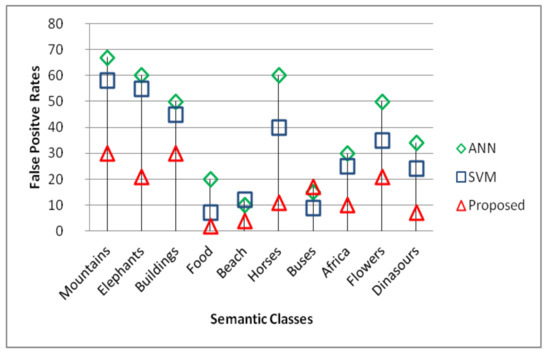
Figure 8.
False positive comparison against ANN and SVM classifiers in terms of false positive rates.
5.4. Performance Evaluation in Imbalanced Domains
The evaluation criteria is the most significant thing for the classifier assessment. The confusion matrix is used in binary classification problems to record the results of correct and incorrect recognitions for a particular classifier through accuracy measure. However, when the data-sets are highly imbalanced the accuracy measure cannot be tuned to verify the performance of a classifier, as it is unable to distinguish the number of correct classifications between the examples of different classes [14]. Therefore, in the imbalanced domain there are some other appropriate matrices that can be considered to measure the classification performance, i.e., [14]:
where the is the true positive rate (also known as sensitivity) that describes the percentage of the positive instances that are classified correctly, is the true negative rate is the percentage of the negative instances correctly classified, is the false positive rate (one-specificity) is the number of negative instances misclassified, and similarly is the false negative rate is the number of positive instances that are misclassified. As the classification is applied with an intention to improve the results, none of the measures mentioned above are appropriate to measure the classification performance individually. One way to generate the combination of these measures is through the receiver operating characteristic (ROC) curves [14], that allows to view the trade-off between the benefits () and cost ().
As in our implementation we are performing the image classification by mapping the multi-class problem in the form of multiple binary classification problems, therefore, we have also evaluated the classification performance through the ROC measure. Classification rates of the proposed method are compared against several existing systems of CBIR in terms of area under the ROC curve (AUC). The comparative methods are those of Kundu et al. [49], Yuan et al. [54], and Ensemble based SVM [42]. Classification performance in terms of ROC curves are plotted in Figure 9 and Figure 10. From the results it can be observed that the classification results of the proposed method are far better then the comparative methods, that clearly shows its reliability and effectiveness.
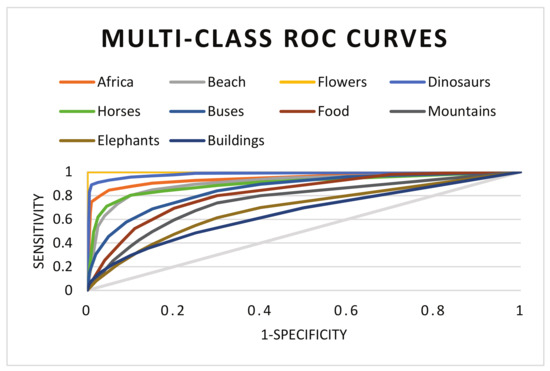
Figure 9.
Comparison of average precision versus rate of returned images.
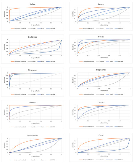
Figure 10.
Performance evaluation of the proposed method with other standard content-based image retrieval (CBIR) systems Kundu et al. [49], Yuan et al. [54], and Ensemble based SVM (EMSVM) [42] using the receiver operating characteristic (ROC) curves.
5.5. Relevance Feedback
Relevance feedback (RF) that is incorporated in our system generates the initial output against a query image on the basis of distance. The user gives the initial feedback by selecting only the relevant or the positive images in the returned output, and the remaining images are considered as negative feedbacks. Asymmetric bagging and symmetric bagging procedures as already described are applied on the positive samples to return genetically diverse chromosomes against the positive samples. Negative samples are considered as the chromosomes that are not diverse and after few generations/iterations they are intended to die. The support vector machines and artificial neural networks are trained on both classes of chromosomes and output is generated. The user iteratively provides the feedback on the output until the desired results are achieved. The complete process of the relevance feedback is provided in Algorithm 5.
| Algorithm 5 The relevance feedback algorithm. |
| Input: Positive set , negative set , weak classifier (SVM), (neural networks), integer = 1 (number of generated classifiers) and the test sample x Output: Classifier |
|
Experimental Details
In our experiments, 300 images are randomly selected and then relevance feedback is automatically performed by the computer. All query relevant images (i.e., images with the same concept as the query) are marked as positive feedback samples and all the other images are marked as negative feedback samples. The current system is tested on top 30 and top 60 images with nine iterations, where the zeroth iteration returns the initial output through a distance measure. The average precision of the 300 query images is used to measure the performance of the RF based image retrieval that can be defined as the ratio of relevant images with respect to the retrieval rate.
The proposed RF method is compared against genetically optimized support vector machines (GOSVM) [27], generalized biased discriminant analysis (GBDA) [55], biased discriminant euclidean embedding (BDEE) [4], and direct kernel biased discriminant analysis (DKBDA) [56]. From the results presented in Figure 11 and Figure 12, we can easily observe that the proposed system has outperformed the comparative systems in terms of precision of output, and most importantly the convergence of the proposed method in earlier iterations is far better then the comparative methods, that clearly means that the user will have a better system experience and need to pass from a few feedback rounds to achieve the desired output.
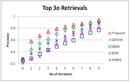
Figure 11.
Comparison of the proposed method in terms of precision on top 30 retrievals against genetically optimized support vector machines (GOSVM), generalized biased discriminant analysis (GBDA), biased discriminant euclidean embedding (BDEE) and direct kernel biased discriminant analysis (DKBDA).
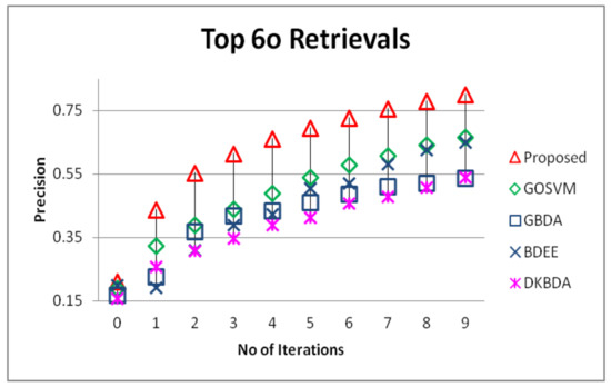
Figure 12.
Comparison of the proposed method in terms of precision on top 60 retrievals against GOSVM, GBDA, BDEE and direct kernel biased discriminant analysis (DKBDA).
5.6. Genetic Algorithm Evaluation
The objective function used in Equation (18) ensures that the GA receives good features in every generation that results in the form of improved classification performance. In order to justify this argument, we have designed an experiment where we compare the classification performance of the proposed method over COIL and Caltech-101 datasets with and without objective function. In the case when the objective function is not used, then we generate a single chromosome population instead of chromosome populations.
From the results presented in Figure 13, we can observe that the objective function with chromosome populations significantly improves the classification performance. The foremost reason behind this improvement in performance is that our objective function suppresses the weak features, hence the under represented class grows with powerful representations and results in improved classification in terms of accuracy measure.
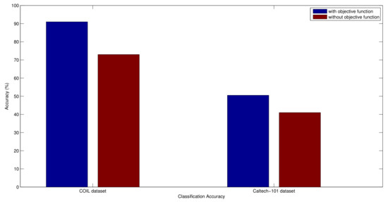
Figure 13.
Average accuracy over COIL and Caltech-101 datasets.
As described in Equation (18), the objective function selects the chromosome population amongst different chromosome populations. In order to evaluate the optimal value for the parameter , we have provided the classification comparison over COIL and Caltech-101 datasets. The results of the comparison are presented in Figure 14. From the results we can observe that the algorithm gain performance benefit in case of COIL dataset with higher values of parameter . Whereas, in case of the Caltech-101 dataset the performance remain constant. The foremost reason behind this performance behaviour is that if the most optimal chromosome population is reached earlier the higher values of parameter will have no impact over the retrieval performance. However, to explore the search space in a better way for obtaining the optimal chromosome population, higher values of parameter are preferred. The impact of higher values of parameter can be observed in case of COIL dataset. Due to this reason the value of parameter in our implementation is set as 500.
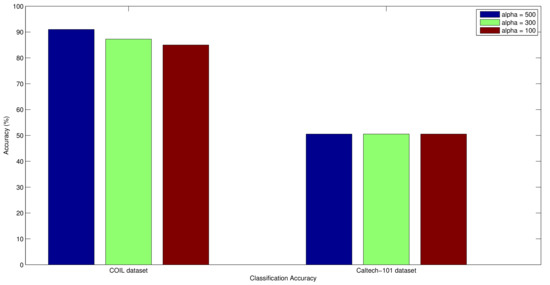
Figure 14.
Average accuracy over COIL and Caltech-101 datasets using different values of parameter .
6. Conclusions
Application of the different classifiers for image classification and retrieval is a well established area of research. However, the classification results are not impressive when datasets suffer from imbalanced class distributions due to the class overlap and small disjuncts. An imbalanced class distribution leads the classifiers to ignore the minority class examples and resultantly lose the classification ability. The severity of the problem increases exponentially when there are several classes enrolled and there exists a high correlation amongst the classes as it is the case in the image classification. To overcome these limitations, a genetic classifier comity learning method is introduced that combines the SVM and ANN learning basis for efficient image retrieval by generating multiple versions of the classifiers through asymmetric and symmetric bagging. To elaborate the effectiveness of our technique, extensive experiments are carried out on the Corel, Caltech-101 and COIL datasets. To measure the semantic association capabilities of the proposed method, we compared it with several popular CBIR techniques. Results show that the proposed method has outperformed the comparative methods, and has also shown promising results in terms of associating images with their right semantic classes.
Acknowledgments
This work was supported by Basic Science Research Program through the National Research Foundation of Korea (NRF) funded by the Ministry of Education (2016R1D1A1B03933860).
Author Contributions
Aun Irtaza, Syed M. Adnan, Khawaja Tehseen Ahmed, Muhammad Tariq Mahmood designed the experiments and analyzed the data. Khawaja Tehseen Ahmed, Ahmad Khan and Ali Javed have developed and implemented the algorithms. Aun Irtaza, Syed M. Adnan, Muhammad Tariq Mahmood and Ali Javed wrote the paper.
Conflicts of Interest
The authors declare no conflict of interest.
References
- Smeulders, A.W.; Worring, M.; Santini, S.; Gupta, A.; Jain, R. Content-based image retrieval at the end of the early years. IEEE Trans. Pattern Anal. Mach. Intell. 2000, 22, 1349–1380. [Google Scholar] [CrossRef]
- Hafiane, A.; Chaudhuri, S.; Seetharaman, G.; Zavidovique, B. Region-based CBIR in GIS with local space filling curves to spatial representation. Pattern Recognit. Lett. 2006, 27, 259–267. [Google Scholar] [CrossRef]
- Chen, X.; Zhang, C. An interactive semantic video mining and retrieval platform—Application in transportation surveillance video for incident detection. In Proceedings of the ICDM’06, IEEE Sixth International Conference on Data Mining, Hong Kong, China, 18–22 December 2006; pp. 129–138. [Google Scholar]
- Bian, W.; Tao, D. Biased discriminant Euclidean embedding for content-based image retrieval. IEEE Trans. Image Process. 2010, 19, 545–554. [Google Scholar] [CrossRef] [PubMed]
- Saadatmand-Tarzjan, M.; Moghaddam, H.A. A novel evolutionary approach for optimizing content-based image indexing algorithms. IEEE Trans. Syst. Man, Cybern. B Cybern. 2007, 37, 139–153. [Google Scholar] [CrossRef]
- Krishnapuram, R.; Medasani, S.; Jung, S.H.; Choi, Y.S.; Balasubramaniam, R. Content-based image retrieval based on a fuzzy approach. IEEE Trans. Knowl. Data Eng. 2004, 16, 1185–1199. [Google Scholar] [CrossRef]
- Demir, B.; Bruzzone, L. A novel active learning method in relevance feedback for content-based remote sensing image retrieval. IEEE Trans. Geosci. Remote Sens. 2015, 53, 2323–2334. [Google Scholar] [CrossRef]
- Ashraf, R.; Bashir, K.; Mahmood, T. Content-based Image Retrieval by Exploring Bandletized Regions through Support Vector Machines. J. Inf. Sci. Eng. 2016, 32, 245–269. [Google Scholar]
- Le, T.M. Clustering Binary Signature Applied in Content-Based Image Retrieval. In New Advances in Information Systems and Technologies; Springer: Cham, Switzerland, 2016; pp. 233–242. [Google Scholar]
- Zhuang, Y.T.; Yang, Y.; Wu, F. Mining semantic correlation of heterogeneous multimedia data for cross-media retrieval. IEEE Trans. Multimedia 2008, 10, 221–229. [Google Scholar] [CrossRef]
- Xue, H.; Chen, S.; Yang, Q. Structural regularized support vector machine: A framework for structural large margin classifier. IEEE Trans. Neural Netw. 2011, 22, 573–587. [Google Scholar] [CrossRef] [PubMed]
- Yan, Y.; Liu, G.; Wang, S.; Zhang, J.; Zheng, K. Graph-based clustering and ranking for diversified image search. Multimed. Syst. 2014, 23, 41–52. [Google Scholar] [CrossRef]
- Wang, S.; Chang, X.; Li, X.; Sheng, Q.Z.; Chen, W. Multi-task Support Vector Machines for Feature Selection with Shared Knowledge Discovery. Signal Process. 2014, 120, 746–753. [Google Scholar] [CrossRef]
- Galar, M.; Fernandez, A.; Barrenechea, E.; Bustince, H.; Herrera, F. A review on ensembles for the class imbalance problem: Bagging-, boosting-, and hybrid-based approaches. IEEE Trans. Syst. Man Cybern. Part C Appl. Rev. 2012, 42, 463–484. [Google Scholar] [CrossRef]
- Irtaza, A.; Jaffar, M.A. Categorical image retrieval through genetically optimized support vector machines (GOSVM) and hybrid texture features. Signal Image Video Process. 2015, 9, 1503–1519. [Google Scholar] [CrossRef]
- Yang, Q.; Wu, X. 10 challenging problems in data mining research. Int. J. Inf. Technol. Decis. Mak. 2006, 5, 597–604. [Google Scholar] [CrossRef]
- Qi, G.J.; Aggarwal, C.; Rui, Y.; Tian, Q.; Chang, S.; Huang, T. Towards cross-category knowledge propagation for learning visual concepts. In Proceedings of the 2011 IEEE Conference on Computer Vision and Pattern Recognition (CVPR), Colorado Springs, CO, USA, 20–25 June 2011; pp. 897–904. [Google Scholar]
- Yang, L.; Gong, W.; Gu, X.; Li, W.; Liu, Y. Bagging null space locality preserving discriminant classifiers for face recognition. Pattern Recognit. 2009, 42, 1853–1858. [Google Scholar] [CrossRef]
- Zhang, Y.; Fu, P.; Liu, W.; Zou, L. SVM classification for imbalanced data using conformal kernel transformation. In Proceedings of the 2014 IEEE International Joint Conference on Neural Networks (IJCNN), Beijing, China, 6–11 July 2014; pp. 2894–2900. [Google Scholar]
- Maratea, A.; Petrosino, A.; Manzo, M. Adjusted F-measure and kernel scaling for imbalanced data learning. Inf. Sci. 2014, 257, 331–341. [Google Scholar] [CrossRef]
- Tao, D.; Tang, X.; Li, X.; Wu, X. Asymmetric bagging and random subspace for support vector machines-based relevance feedback in image retrieval. IEEE Trans. Pattern Anal. Mach. Intell. 2006, 28, 1088–1099. [Google Scholar] [PubMed]
- Wang, X.Y.; Chen, J.W.; Yang, H.Y. A new integrated SVM classifiers for relevance feedback content-based image retrieval using EM parameter estimation. Appl. Soft Comput. 2011, 11, 2787–2804. [Google Scholar] [CrossRef]
- Chang, E.Y. Imbalanced Data Learning. In Foundations of Large-Scale Multimedia Information Management and Retrieval; Springer: New York, NY, USA, 2011; pp. 191–211. [Google Scholar]
- Yuan, B.; Ma, X. Sampling+ reweighting: Boosting the performance of AdaBoost on imbalanced datasets. In Proceedings of the 2012 IEEE International Joint Conference on Neural Networks (IJCNN), Brisbane, Australia, 10–15 June 2012; pp. 1–6. [Google Scholar]
- Belattar, K.; Mostefai, S.; Draa, A. A Hybrid GA-LDA Scheme for Feature Selection in Content-Based Image Retrieval. Int. J. Appl. Metaheuristic Comput. 2018, 9, 48–71. [Google Scholar] [CrossRef]
- Luong, A.V.; Nguyen, T.T.; Pham, X.C.; Nguyen, T.T.T.; Liew, A.W.C.; Stantic, B. Automatic Image Region Annotation by Genetic Algorithm-Based Joint Classifier and Feature Selection in Ensemble System. In Intelligent Information and Database Systems, Proceedings of the 10th Asian Conference on Intelligent Information and Database Systems, Dong Hoi City, Vietnam, 19–21 March 2018; Springer: Cham, Switzerland, 2018; pp. 599–609. [Google Scholar]
- Irtaza, A.; Jaffar, M.A.; Muhammad, M.S. Content based image retrieval in a web 3.0 environment. Multimed. Tools Appl. 2015, 74, 5055–5072. [Google Scholar] [CrossRef]
- Wang, S.; Yao, X. Multiclass imbalance problems: Analysis and potential solutions. IEEE Trans. Syst. Man, Cybern B, Cybern. 2012, 42, 1119–1130. [Google Scholar] [CrossRef] [PubMed]
- Galar, M.; Fernández, A.; Barrenechea, E.; Herrera, F. Eusboost: Enhancing ensembles for highly imbalanced data-sets by evolutionary undersampling. Pattern Recognit. 2013, 46, 3460–3471. [Google Scholar] [CrossRef]
- Lam, L.; Suen, C.Y. Optimal combinations of pattern classifiers. Pattern Recognit. Lett. 1995, 16, 945–954. [Google Scholar] [CrossRef]
- Dietterich, T.G. Ensemble Methods in Machine Learning. In Multiple Classifier Systems. MCS 2000. Lecture Notes in Computer Science; Springer: Berlin/Heidelberg, Germany, 2000; Volume 1857, pp. 1–15. [Google Scholar]
- Meynet, J. Information Theoretic Combination of Classifiers with Application to Face Detection. Ph.D. Thesis, Pennsylvania State University, Pennsylvania, PA, USA, 2007. [Google Scholar]
- Breiman, L. Bagging predictors. Mach. Learn. 1996, 24, 123–140. [Google Scholar] [CrossRef]
- Oza, N.C.; Tumer, K. Classifier ensembles: Select real-world applications. Inf. Fusion 2008, 9, 4–20. [Google Scholar] [CrossRef]
- Ma, J.; Plonka, G. The curvelet transform. IEEE Signal Process. Mag. 2010, 27, 118–133. [Google Scholar] [CrossRef]
- Zhang, J.; Wang, Y. A comparative study of wavelet and curvelet transform for face recognition. In Proceedings of the 3rd International Congress on Image and Signal Processing (CISP), Yantai, China, 16–18 October 2010; Volume 4, pp. 1718–1722. [Google Scholar]
- Herrera, F.; Lozano, M.; Sánchez, A.M. Hybrid crossover operators for real-coded genetic algorithms: An experimental study. Soft Comput. 2005, 9, 280–298. [Google Scholar] [CrossRef]
- Arevalillo-Herráez, M.; Ferri, F.J.; Moreno-Picot, S. Distance-based relevance feedback using a hybrid interactive genetic algorithm for image retrieval. Appl. Soft Comput. 2011, 11, 1782–1791. [Google Scholar] [CrossRef]
- Stejić, Z.; Takama, Y.; Hirota, K. Genetic algorithm-based relevance feedback for image retrieval using local similarity patterns. Inf. Process. Manag. 2003, 39, 1–23. [Google Scholar] [CrossRef]
- Weber, M.; Crilly, P.; Blass, W.E. Adaptive noise filtering using an error-backpropagation neural network. IEEE Trans. Instrum. Meas. 1991, 40, 820–825. [Google Scholar] [CrossRef]
- Lai, C.C.; Chen, Y.C. A user-oriented image retrieval system based on interactive genetic algorithm. IEEE Trans. Instrum. Meas. 2011, 60, 3318–3325. [Google Scholar] [CrossRef]
- Yildizer, E.; Balci, A.M.; Hassan, M.; Alhajj, R. Efficient content-based image retrieval using multiple support vector machines ensemble. Expert Syst. Appl. 2012, 39, 2385–2396. [Google Scholar] [CrossRef]
- Youssef, S.M. ICTEDCT-CBIR: Integrating curvelet transform with enhanced dominant colors extraction and texture analysis for efficient content-based image retrieval. Comput. Electr. Eng. 2012, 38, 1358–1376. [Google Scholar] [CrossRef]
- Han, K.; Rezende, R.S.; Ham, B.; Wong, K.Y.K.; Cho, M.; Schmid, C.; Ponce, J. SCNet: Learning Semantic Correspondence. arXiv, 2017; arXiv:1705.04043. [Google Scholar]
- Dubey, S.R.; Singh, S.K.; Singh, R.K. Multichannel decoded local binary patterns for content-based image retrieval. IEEE Trans. Image Process. 2016, 25, 4018–4032. [Google Scholar] [CrossRef] [PubMed]
- Xiao, Y.; Wu, J.; Yuan, J. mCENTRIST: A multi-channel feature generation mechanism for scene categorization. IEEE Trans. Image Process. 2014, 23, 823–836. [Google Scholar] [CrossRef] [PubMed]
- Zhou, Y.; Zeng, F.Z.; Zhao, H.M.; Murray, P.; Ren, J. Hierarchical visual perception and two-dimensional compressive sensing for effective content-based color image retrieval. Cogn. Comput. 2016, 5, 877–889. [Google Scholar] [CrossRef]
- Shrivastava, N.; Tyagi, V. An efficient technique for retrieval of color images in large databases. Comput. Electr. Eng. 2015, 46, 314–327. [Google Scholar] [CrossRef]
- Kundu, M.K.; Chowdhury, M.; Bulò, S.R. A graph-based relevance feedback mechanism in content-based image retrieval. Knowl. Based Syst. 2015, 73, 254–264. [Google Scholar] [CrossRef]
- Zeng, S.; Huang, R.; Wang, H.; Kang, Z. Image retrieval using spatiograms of colors quantized by Gaussian Mixture Models. Neurocomputing 2016, 171, 673–684. [Google Scholar] [CrossRef]
- Walia, E.; Pal, A. Fusion framework for effective color image retrieval. J. Vis. Commun. Image Represent. 2014, 25, 1335–1348. [Google Scholar] [CrossRef]
- Ashraf, R.; Bashir, K.; Irtaza, A.; Mahmood, M.T. Content based image retrieval using embedded neural networks with bandletized regions. Entropy 2015, 17, 3552–3580. [Google Scholar] [CrossRef]
- ElAlami, M.E. A new matching strategy for content based image retrieval system. Appl. Soft Comput. 2014, 14, 407–418. [Google Scholar] [CrossRef]
- Yuan, X.; Yu, J.; Qin, Z.; Wan, T. A SIFT-LBP image retrieval model based on bag of features. In Proceedings of the IEEE International Conference on Image Processing, Brussels, Belgium, 11–14 September 2011. [Google Scholar]
- Zhang, L.; Wang, L.; Lin, W. Generalized biased discriminant analysis for content-based image retrieval. IEEE Trans. Syst. Man, Cybern B, Cybern. 2012, 42, 282–290. [Google Scholar] [CrossRef] [PubMed]
- Tao, D.; Tang, X.; Li, X.; Rui, Y. Direct kernel biased discriminant analysis: A new content-based image retrieval relevance feedback algorithm. IEEE Trans. Multimed. 2006, 8, 716–727. [Google Scholar]
© 2018 by the authors. Licensee MDPI, Basel, Switzerland. This article is an open access article distributed under the terms and conditions of the Creative Commons Attribution (CC BY) license (http://creativecommons.org/licenses/by/4.0/).