Modeling Restrained Shrinkage Induced Cracking in Concrete Rings Using the Thick Level Set Approach

Abstract

Modeling restrained shrinkage-induced damage and cracking in concrete is addressed herein. The novel Thick Level Set (TLS) damage growth and crack propagation model is used and adapted by introducing shrinkage contribution into the formulation. The TLS capacity to predict damage evolution, crack initiation and growth triggered by restrained shrinkage in absence of external loads is evaluated. A study dealing with shrinkage-induced cracking in elliptical concrete rings is presented herein. Key results such as the effect of rings oblateness on stress distribution and critical shrinkage strain needed to initiate damage are highlighted. In addition, crack positions are compared to those observed in experiments and are found satisfactory.

1. Introduction

Shrinkage, a time-dependent volumetric change, is a complex material response affecting concrete in an adverse manner. Several factors impact concrete drying such as relative humidity, exposed drying surface, cement characteristics, shape and even the size of the structure. It is important to distinguish between plastic shrinkage, autogenous shrinkage and drying shrinkage. The first occurs while the concrete is still wet and may generate significant cracking during the setting phase. Plastic shrinkage is particularly a concern when using high strength concrete; the reinforcements are ineffective during the setting phase. The second, usually quantified using sealed specimens, is a result of various chemical reactions and self-desiccation leading to water loss due to the hydration reaction. The third is caused by the loss of water during the drying process. Concrete shrinkage strain is the sum of both the autogenous and drying shrinkage strains. It is an increasing function of time with a decreasing rate. For the sake of clarity, shrinkage strain is used when talking about the total shrinkage strain in the remainder of this paper.

Despite decades of research, shrinkage remains an important property to be controlled. To be more precise, unrestrained shrinkage, where the material is free to shrink, does not generate stresses and is hence not a major concern for structural engineering. In reality, the concrete structural elements are rarely, if ever, free to shrink; they can be restrained by their support, by the adjacent members or even by any bonded reinforcement. Consequently, shrinkage introduces a heterogeneous stress field leading to damage development when exceeding the concrete tensile strength. This threatens the integrity of the concrete structures and leads to their premature failure. It could be translated by an increase of permeability for structures such as dams, tanks and containment vessels or a decrease of performance for structures such as tunnels and bridges.

It should be noted that ‘free’ shrinkage estimations are not enough for evaluating cracking tendencies. In other words and although shrinkage data are a major actor, it does not determine how the concrete will behave during service [1]. For this reason, concrete damage and cracking tendencies are normally evaluated under different restrained conditions via a series of cracking tests such as slab, bar and ring tests. The latter is wide-spread due to its simplicity and versatility and it is also adopted in the present study. A great deal of researchers have investigated cracking in circular ring tests under different restrained conditions. Their work covered everything starting with the effect of the used mixture [2,3,4,5,6,7], the ring size/geometry [8,9,10], the drying conditions [5,8,11] and even the restraining steel ring wall thickness [12] on the concrete cracking tendencies. Consequently, the circular ring test became a standard testing method recommended by the AASHTO and ASTM in 2005 [13,14].

Despite the simplicity and adaptability of the circular ring test, the authors of [8,9,15] highlighted key challenges summarized by the long time (up to one month) needed to develop a visible crack and the high dependency on the restraining steel stiffness.

Solving the latter problems as an objective in mind, the authors of [16] proposed a variation of the ring test by adopting elliptical rings instead. In later works [17,18], the study was extended to a wider range of specimens covering also thin and thick ring geometries. Using elliptical rings yielded a shorter period to generate visible cracks. In addition, the measuring instruments’ cost is reduced since the cracks’ positions are concentrated in known positions unlike circular rings (where the cracks have an equal opportunity to be initiated all over the circumference). Despite the appeal of using elliptical rings instead of circular ones, not much effort (besides the just mentioned works) has been made to validate and approve/disapprove of the advantages of using elliptical geometries.

From the modeling point of view, even less works dedicated to restrained shrinkage-induced cracking in concrete rings are found in the literature. We cite for instance the work of [11,19,20,21], proposing theoretical/analytical models to estimate the cracking age of concrete and the residual stress development. These models, despite their simplicity, showed good estimations. Unfortunately, the same equations are not well adapted when dealing with elliptical rings. The same authors who initially proposed the elliptical ring test proposed in their newest work [17] a fracture mechanics-based numerical approach using the R-curve method to predict crack initiation in restrained concrete elliptical rings. The latter uses notched elliptical rings with an initial crack located on the major axis. The cracking ages matched the ones found experimentally. None of the above models can offer a complete scenario starting from a sound to partially damaged then to fully damaged ring. In addition, no information about the crack path and its evolution is available.

The present work is a first attempt using the promising Thick Level Set approach (TLS), a regularized damage model with automatic transition to fracture [22,23,24,25], to model damage evolution and crack propagation in concrete structures due to restrained shrinkage. The TLS model acts as a bridge between damage mechanics and fracture mechanics. Starting from a perfectly sound material, an initial damage can be detected automatically. Once the material is fully degraded in a zone, a crack is automatically initiated. Crack branching and interactions are straightforwardly handled as well.

A brief description of the TLS damage model is presented in Section 2 with a special emphasis on the time-independent evolution law adopted in this work (see Section 2.1), as well as on the shrinkage contribution (see Section 2.1). Following the promising preliminary results presented in [26], the study dealing with shrinkage-induced cracking in elliptical concrete rings is extended in Section 3. The effect of ring geometry, more precisely rings’ oblateness, is investigated. Numerical results issued by the TLS are analyzed. Crack positions are superposed on those obtained in [17,27]. The capacity of this novel TLS model is evaluated for concrete applications. Ideas for future generalization and enrichment are thus proposed accordingly in Section 4.

2. Thick Level Set Damage Model

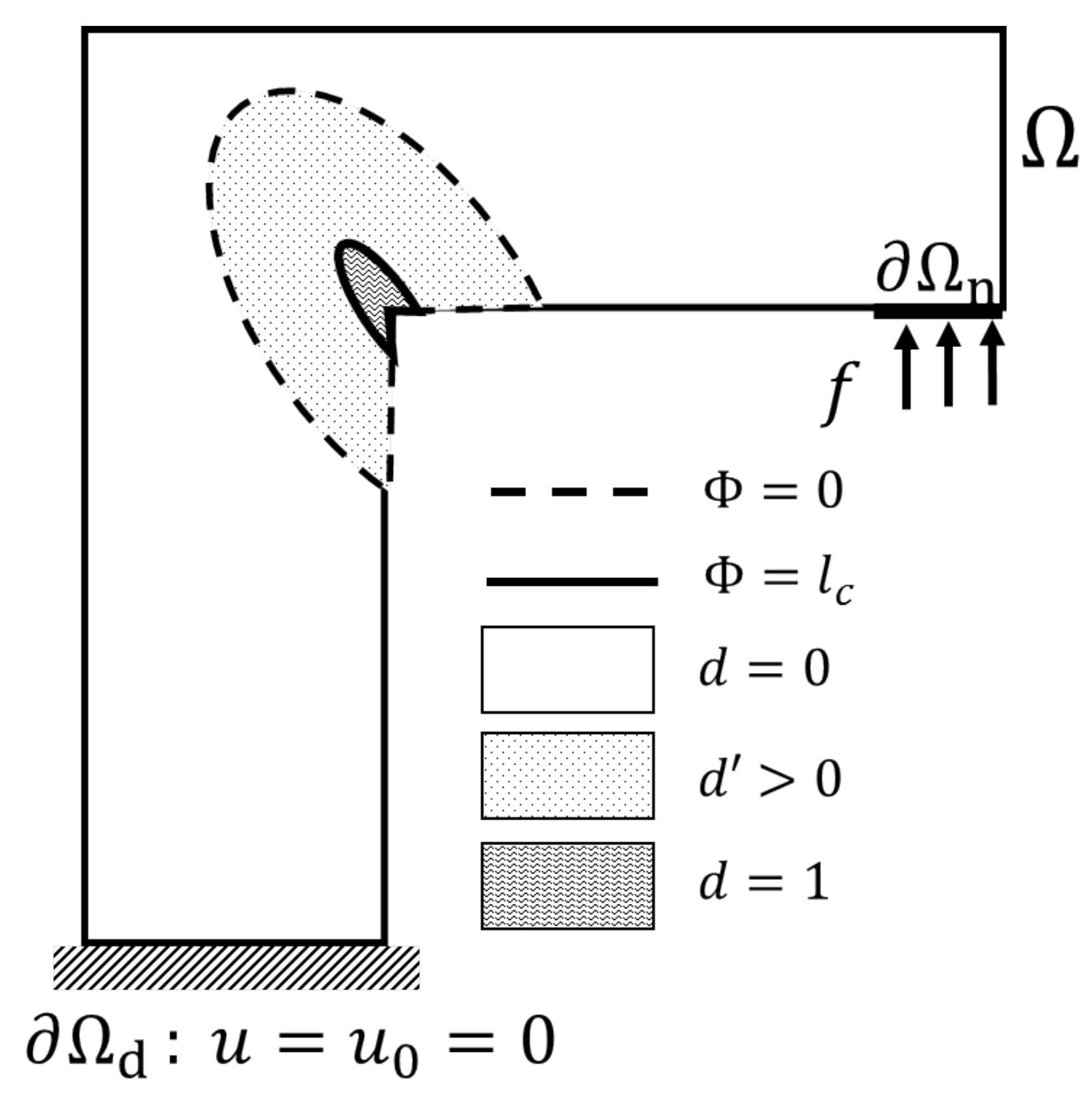
The thick level set model is a new theoretical damage model offering a natural and easy way to transition from damage to fracture. It straightforwardly treats crack initiation and interaction such as coalescence and branching [23]. Both sound and damaged zones are described implicitly using a single level set function and a characteristic material-dependent thickness $l_c$. The damage is an increasing function of this signed distance $\mathsf{\Phi }$ and is expressed as follows:

$$\left\{\begin{array}{ccccc}d\left(\mathsf{\Phi }\right)\hfill & =& 0\hfill & if\hfill & \mathsf{\Phi }\le 0\hfill \\ d^{\prime }\left(\mathsf{\Phi }\right)\hfill & \ge & 0\hfill & if\hfill & 0\le \mathsf{\Phi }\le l_c\hfill \\ d\left(\mathsf{\Phi }\right)\hfill & =& 1\hfill & if\hfill & \mathsf{\Phi }\ge l_c\hfill \end{array}\right.$$

(1)

In other words, the zero-isovalue of $\mathsf{\Phi }$ delimits the sound ($d=0$) from the partially-damaged zone ($d^{\prime }>0$), whereas the $l_c$-isovalue delimits the partially- from the fully-damaged zone ($d=1$). When $l_c$ is reached, a crack is initiated, as illustrated in Figure 1.

By introducing the characteristic length $l_c$ and a damage function $d\left(\mathsf{\Phi }\right)$, the TLS model does not only ensure a transition between damage and cracking, but acts as a regularization method to solve spurious mesh dependencies when strain softening occurs (see Section 2.2).

2.1. Local Governing Equations and Time-Independent Damage Evolution Law

Under the assumptions of small strains and displacements, the following set of equations is solved:

$$\left\{\begin{array}{ccccc}\nabla .\sigma \hfill & =& 0\hfill & on\hfill & \mathsf{\Omega }\hfill \\ \sigma .n\hfill & =& f\hfill & on\hfill & \partial {\mathsf{\Omega }}_n\hfill \\ u\hfill & =& u_0\hfill & on\hfill & \partial {\mathsf{\Omega }}_d\hfill \end{array}\right.$$

(2)

where $\sigma$ is the Cauchy stress tensor, u the displacement vector, f an external load applied on $\partial {\mathsf{\Omega }}_n$, n the normal vector and $u_0$ prescribed displacements imposed on $\partial {\mathsf{\Omega }}_d$.

Defining a free energy W, the stress tensor $\sigma$ and the energy release rate Y can be related to the strain tensor and the damage as follows:

$$\left\{\begin{array}{ccc}\sigma \hfill & =& \frac{\partial W(\epsilon ,d)}{\partial \epsilon }\hfill \\ Y\hfill & =& -\frac{\partial W(\epsilon ,d)}{\partial d}\hfill \end{array}\right.$$

(3)

In the present paper, we use a free energy form W reflecting the concrete dissymmetric behavior in tension and compression:

$$W(\epsilon ,d)=\mu (1-{\alpha }_{i}d){\epsilon }_i^2+\frac{\lambda }{2}(1-\alpha d)tr{\left(\epsilon \right)}^2$$

(4)

where ${\epsilon }_i$ are the eigenvalues of $\epsilon$, $\mu$ and $\lambda$ are Lamé coefficients and $\alpha$ and ${\alpha }_i$ are two parameters ensuring the dissymmetric behavior: $\alpha =\left\{\begin{array}{ccc}0\hfill & if& tr\left(\epsilon \right)<0\hfill \\ 1\hfill & if& tr\left(\epsilon \right)\ge 0\hfill \end{array}\right.\mathrm{and}{\alpha }_i=\left\{\begin{array}{ccc}0\hfill & if& {\epsilon }_i<0\hfill \\ 1\hfill & if& {\epsilon }_i\ge 0\hfill \end{array}\right.$.

As for the local damage evolution law [22,23,24,25], a time-independent law is adopted where the damage grows when Y reaches the critical energy release rate $Y_c$:

$$Y-Y_c\le 0;\dot{d}\ge 0;(Y-Y_c)\dot{d}=0$$

(5)

2.2. Energetic form and Regularization

The system of Equations (2) can be alternatively expressed using the energetic formulation.

If P denotes the potential energy, the variational form is obtained by minimizing P with respect to $\delta u$ and $\delta \mathsf{\Phi }$:

$$P(u,\mathsf{\Phi })={\int }_{\mathsf{\Omega }}W(\epsilon \left(u\right),d\left(\mathsf{\Phi }\right))d\mathsf{\Omega }-{\int }_{\partial {\mathsf{\Omega }}_n}f.ud\partial \mathsf{\Omega }$$

(6)

Using the relation $\delta W=\frac{\partial W}{\partial \epsilon }\delta \epsilon +\frac{\partial W}{\partial d}\delta d$, the potential energy P can be differentiated as follows:

$$DP(u,\mathsf{\Phi })\left[(\delta u,\delta \mathsf{\Phi })\right]={\int }_{\mathsf{\Omega }}\sigma :\epsilon \left(\delta u\right)d\mathsf{\Omega }-{\int }_{\partial {\mathsf{\Omega }}_n}f.\delta ud\partial \mathsf{\Omega }-{\int }_{\mathsf{\Omega }}Y{d}^{\prime }\left(\mathsf{\Phi }\right)\delta \mathsf{\Phi }d\mathsf{\Omega }$$

(7)

The equilibrium equation is obtained by zeroing (7) with respect to $(\delta u,0)$:

$$DP(u,\mathsf{\Phi })\left[(\delta u,0)\right]={\int }_{\mathsf{\Omega }}\sigma :\epsilon \left(\delta u\right)d\mathsf{\Omega }-{\int }_{\partial {\mathsf{\Omega }}_n}f.\delta ud\partial \mathsf{\Omega }=0$$

(8)

The amount of dissipated energy as the front moves is obtained by analyzing (7) for $(0,\delta \mathsf{\Phi })$:

$$DP(u,\mathsf{\Phi })\left[(0,\delta \mathsf{\Phi })\right]=-{\int }_{\mathsf{\Omega }}Y{d}^{\prime }\left(\mathsf{\Phi }\right)\delta \mathsf{\Phi }d\mathsf{\Omega }$$

(9)

The variational problem defined above is known to face issues such as spurious mesh dependencies. The latter may provoke damage growth with negligible energy. Regularization methods are used to prevent such problems.

The TLS model, by definition (1), is a regularization method using the characteristic length $l_c$ to bound the damage evolution to the band limited by $\mathsf{\Phi }=l_c$. In addition and since the damage derivative $d^{\prime }\left(\mathsf{\Phi }\right)$ is non-zero only in the damaged zone (i.e., $0<\mathsf{\Phi }\le l_c$), the integration is limited to the damaged band unlike other non-local classical damage models. Thus, the regularization and the “non-local” treatment of the TLS are activated only on this damaged band.

In addition, a change of variables can be introduced. The dissipated energy in the new basis $(\mathsf{\Phi },s)$ is hence expressed as:

$$DP(u,\mathsf{\Phi })\left[(0,\delta \mathsf{\Phi })\right]=-{\int }_{{\Gamma }_0}{\int }_0^{0\le l\le l_c}Y(\mathsf{\Phi },s)d^{\prime }\left(\mathsf{\Phi }\right)\left(1-\mathsf{\Phi }/\rho \left(s\right)\right)d\mathsf{\Phi }\delta \mathsf{\Phi }ds$$

(10)

where s and $\rho$ are respectively the curvilinear coordinate and the curvature radius along ${\Gamma }_0$. The latter is the boundary corresponding to the zero-isovalue of $\mathsf{\Phi }$.

Damage growth is then activated when:

$${\int }_{{\Gamma }_0}{\int }_0^{0\le l\le l_c}Y(\mathsf{\Phi },s)d^{\prime }\left(\mathsf{\Phi }\right)\left(1-\mathsf{\Phi }/\rho \left(s\right)\right)d\mathsf{\Phi }\delta \mathsf{\Phi }ds={\int }_{{\Gamma }_0}{\int }_0^{0\le l\le l_c}{Y}_c(\mathsf{\Phi },s)d^{\prime }\left(\mathsf{\Phi }\right)\left(1-\mathsf{\Phi }/\rho \left(s\right)\right)d\mathsf{\Phi }\delta \mathsf{\Phi }ds$$

(11)

Regarding the regularization, the authors of [22] propose averaging Y and $Y_c$ by introducing the homogenized quantities $\overline{Y}$ and ${\overline{Y}}_c$:

$$\begin{array}{cc}\overline{Y}=\frac{{\int }_0^{0\le l\le l_c}Y(\mathsf{\Phi },s)d^{\prime }\left(\mathsf{\Phi }\right)(1-\mathsf{\Phi }/\rho \left(s\right))d\mathsf{\Phi }}{{\int }_0^{0\le l\le l_c}{d}^{\prime }\left(\mathsf{\Phi }\right)(1-\mathsf{\Phi }/\rho \left(s\right))d\mathsf{\Phi }}\hfill & {\overline{Y}}_c=\frac{{\int }_0^{0\le l\le l_c}{Y}_c(\mathsf{\Phi },s)d^{\prime }\left(\mathsf{\Phi }\right)(1-\mathsf{\Phi }/\rho \left(s\right))d\mathsf{\Phi }}{{\int }_0^{0\le l\le l_c}{d}^{\prime }\left(\mathsf{\Phi }\right)(1-\mathsf{\Phi }/\rho \left(s\right))d\mathsf{\Phi }}\hfill \end{array}$$

(12)

Note that if $Y_c$ is uniform all over the domain and independent of d; ${\overline{Y}}_c=Y_c$. The new homogenized quantities fulfill the propagation condition; the regularized front evolution reads:

$$\overline{Y}-{\overline{Y}}_c\le 0;\dot{a}\ge 0;(\overline{Y}-{\overline{Y}}_c)\dot{a}=0$$

(13)

where a denotes the front advance to be computed as described in Section 2.4, Figure 2.

Adopting this strategy means that non-locality appears only when $d>0$ and that the non-local model tends to the local model when $l_c$ tends to zero:

$$\underset{l_c\to 0}{lim}\overline{Y}=Y\mathrm{and}\underset{l_c\to 0}{lim}{\overline{Y}}_c=Y_c$$

(14)

2.3. Shrinkage Contribution

To estimate the shrinkage strain, most studies in the literature neglect the heterogeneous nature of the concrete and its effect on the drying process. Semi-analytical and empirical models such as Eurocode [28] and the B3 model [29] provide a good approximation of the shrinkage evolution with time taking into account concrete composition, ambient humidity, geometry, drying surface area-to-volume (A/V) ratio and much more. These approximations are mean values per cross-section. In the present paper, the same logic is adopted. This point will be revisited in future works to reflect reality by computing heterogeneous shrinkage strain fields. Note that, in the present paper, free shrinkage data issued from experimental measurements are used exactly in the same manner.

The total strain is expressed as the sum of the shrinkage strain and the mechanical one $\epsilon ={\epsilon }^{shr}+{\epsilon }^{mec}$. In other words, the mechanical strain is the sole responsible of generating (or not) stresses.

Therefore, taking into account the shrinkage into the TLS formulation is equivalent to writing:

$$\left\{\begin{array}{ccc}\sigma \hfill & =& \frac{\partial W(\epsilon -{\epsilon }^{shr},d)}{\partial \epsilon }\hfill \\ Y\hfill & =& -\frac{\partial W(\epsilon -{\epsilon }^{shr},d)}{\partial d}\hfill \end{array}\right.$$

(15)

with ${\epsilon }^{shr}=\left(\begin{array}{ccc}{\epsilon }_{\infty }^{shr}& 0& 0\\ 0& {\epsilon }_{\infty }^{shr}& 0\\ 0& 0& {\epsilon }_{\infty }^{shr}\end{array}\right)$ and ${\epsilon }_{\infty }^{shr}$ being the shrinkage strain when $t\to \infty$.

Although the considered shrinkage strain is the one reached after an infinite drying time (i.e., maximum), another drying time could be as easily considered.

When writing the variational formulation, considering shrinkage introduces additional volume integrations in Equations (8) and (9).

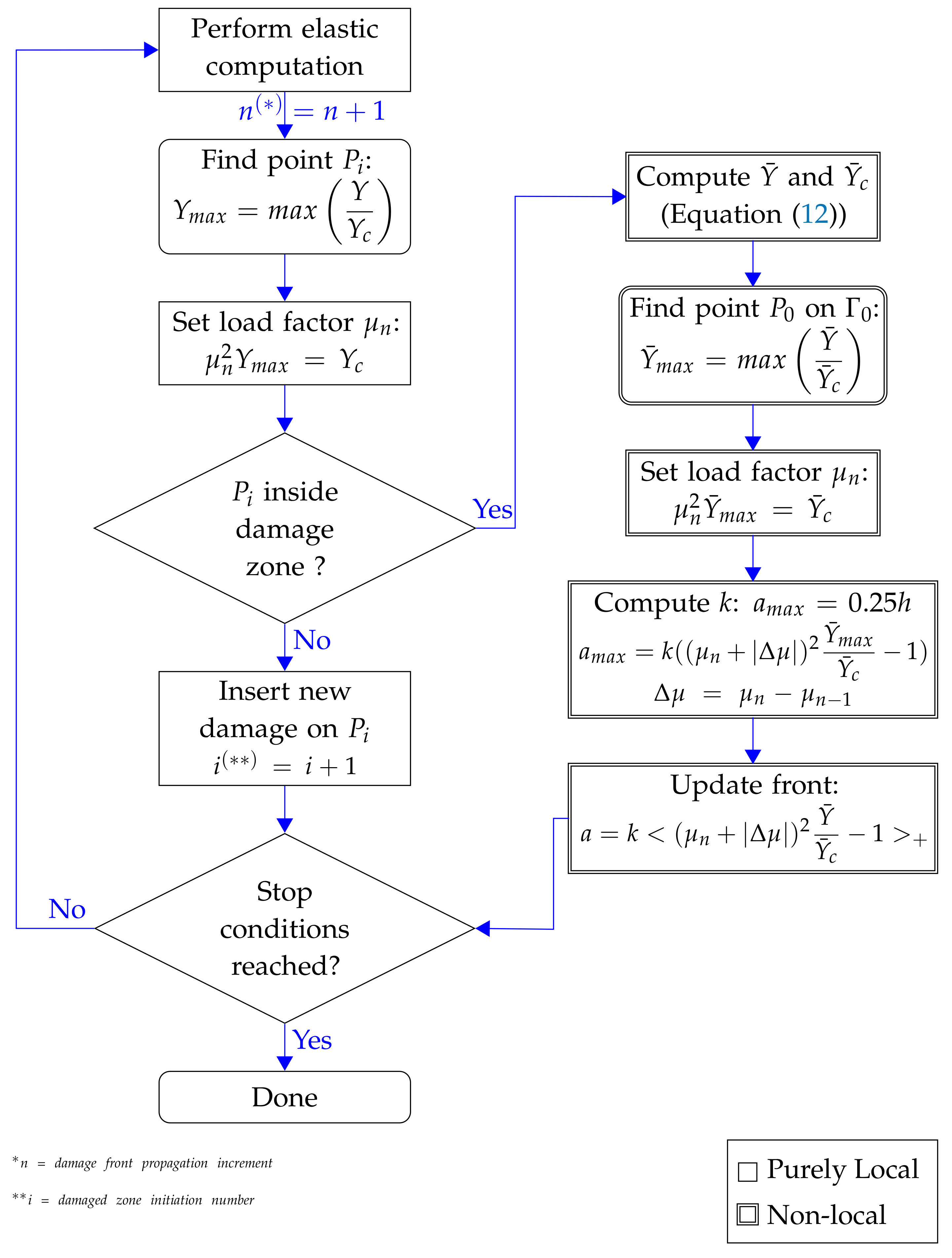
2.4. Staggered Iterative Algorithm

In this work, a staggered explicit approach is adopted for more robustness and computational efficiency by decoupling the elastic computation and the damage front propagation. The computation of damage initiation and propagation at each step is summarized in the flowchart depicted in Figure 2.

First, elastic fields are computed enforcing the equilibrium for a specific loading factor $\mu$. The latter is obtained to obey $max\left(Y\right)=Y_c$. Based on these fields, the damage criterion is evaluated, and front propagation is computed/updated using a time-independent approach.

The front advance $a_{max}$ cannot exceed a predefined factor of the mesh size h to ensure consistency between different steps and prevent stability issues; the parameter k used in the front update and load factor increments ${\mu }_n$ are computed accordingly. Front advance is almost proportional to $<\overline{Y}-{\overline{Y}}_c{>}_{+}$, ensuring the damage irreversibility. Although damage initiation is purely local, the following stages (such as damage evolution, crack initiation and propagation) are treated non-locally, avoiding thus spurious problems related to mesh dependencies. The readers are invited to read [22] for in-depth detail on how to determine k and ${\mu }_n$.

2.5. On the Choice of TLS Parameters

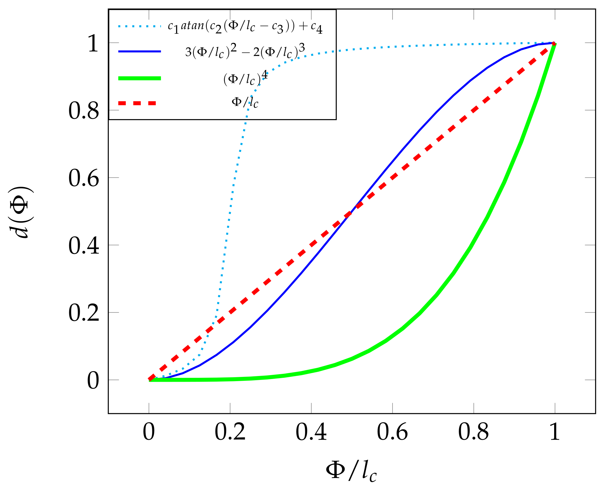
The TLS model is a model with few, but very important parameters to be chosen properly. In fact, only three parameters need to be identified: (i) the damage profile with respect to the level set $d\left(\mathsf{\Phi }\right)$; (ii) the characteristic length $l_c$ ; and (iii) the critical energy release rate $Y_c$. Several approaches can be adopted to do so. In the present study, the adopted approach relies on confronting the TLS model with fracture mechanics.

We start by fixing the damage profile $d\left(\mathsf{\Phi }\right)$. Several choices are illustrated in Figure 3. Although the choices are countless, the damage profile is chosen to be a good fit and true to the targeted application. Choosing for instance the fourth order polynomial profile $d\left(\mathsf{\Phi }\right)={(\frac{\mathsf{\Phi }}{l_c})}^4$ yields a short almost non-existent process zone ahead of the crack tip. One could easily explore more sophisticated profiles such as the arc-tangent profile $d\left(\mathsf{\Phi }\right)=c_{1}atan(c_2(\frac{\mathsf{\Phi }}{l_c}-c_3))+c_4$, illustrating a longer process zone, but should keep in mind that such profiles are tricky to handle. They introduce more parameters ${\left(c_i\right)}_{i\in \{1,2,3,4\}}$ to be identified and might face numerical integration problems due to the large slack zone. The third order polynomial profile $d\left(\mathsf{\Phi }\right)=3{(\frac{\mathsf{\Phi }}{l_c})}^2-{(\frac{\mathsf{\Phi }}{l_c})}^3$ is a good intermediate and is adopted throughout this paper following several tests performed prior to this study.

Next, for a given fracture energy $G_c$, a couple $(Y_c,l_c)$ is identified using the relation proven in [23]:

$$G_c=2A{Y}_c{l}_c$$

(16)

with A being the area under the curve $d\left(\mathsf{\Phi }\right)$: $A={\int }_0^{l_c}d\left(\mathsf{\Phi }\right)d\mathsf{\Phi }$.

In other words, every couple $(Y_c,l_c)$ verifying the above relation leads to the same dissipated energy and the same load-CMOD curve. Generally, the characteristic length $l_c$ is chosen to respect $l_c=3.ag{g}_{max}$ where $ag{g}_{max}$ is the maximum aggregate size.

Note that although the mesh size h is not a parameter of the model, it is highly recommended to chose it significantly smaller than the characteristic length $l_c$ in the problematic zone ($h\le 4.l_c$). This ensures the best representation of the transition between the damage and crack initiation.

3. Results

Inspired by the study presented in [17,27], highlighting the effects of the ring geometry on the stress development and consequently crack initiation, similar test cases are proposed.

Figure 4 sketches the ring geometry. To switch from a circular ring to slightly and extremely elliptical rings, we play with the ratio $\frac{a}{b}$; the ring is circular if $\frac{a}{b}=1$ and elliptical otherwise.

Five different ratios are proposed herein. The inner major radius a is always kept equal to 150 mm, while the minor inner radius $b\in \{150;125;100;75;60\}$ mm with a wall thickness $\Delta R$ of $37.5$ mm. All rings share the same height H, equal to 75 mm.

The TLS model treats damage and crack growth at the macroscopic scale. Therefore, only the homogenized properties are needed. To achieve a normal strength concrete, the authors of [17,27] used the following mixture proportions (summarized in

Table 1. Mixture proportions by weight.

Mixture Identification	Cement	Sand	Gravel	Water
w/c = 0.5	1	1.5	1.5	0.5

) with commercially available CEM II Portland cement and a maximum aggregate size $ag{g}_{max}$ of 10 mm.

Based on their regression fit to measurements, Young’s modulus E and Poisson’s ratio $\nu$ are respectively equal to $15.915$ GPa and $0.2$. Note that Day 15 was chosen to retrieve the latter properties since it is approximately the day for which the concrete rings cracked.

When preparing the different rings for the experimental study, they were restricted by inner steel rings, and a coat of a release agent was applied to eliminate friction between concrete and steel. For now, these conditions are imposed by applying directly appropriate conditions on the inner surface of the concrete ring ($u_x=0$, $u_y=0$ and $u_z$ free). This point will be revisited in future works, but remains for now the simplest way to treat the restricted shrinkage without treating contact and friction for multi-material problems.

We start by choosing $l_c=0.03$ m $\simeq 3.ag{g}_{max}$. For a fracture energy $G_c$ of approximately 8.4956 N/m, the value $Y_c$ = 283.18 Pa is chosen to respect Equation (16) as explained earlier.

To bring to light the effects of shrinkage in absence of any external loading, no external load is applied ($f=0$), and we impose a uniform shrinkage strain all over the domain $\mu {\epsilon }^{shr}=\left(\begin{array}{ccc}-\mu & 0& 0\\ 0& -\mu & 0\\ 0& 0& -\mu \end{array}\right)$, where $\mu$ is the load factor to be computed as explained in Section 2.4.

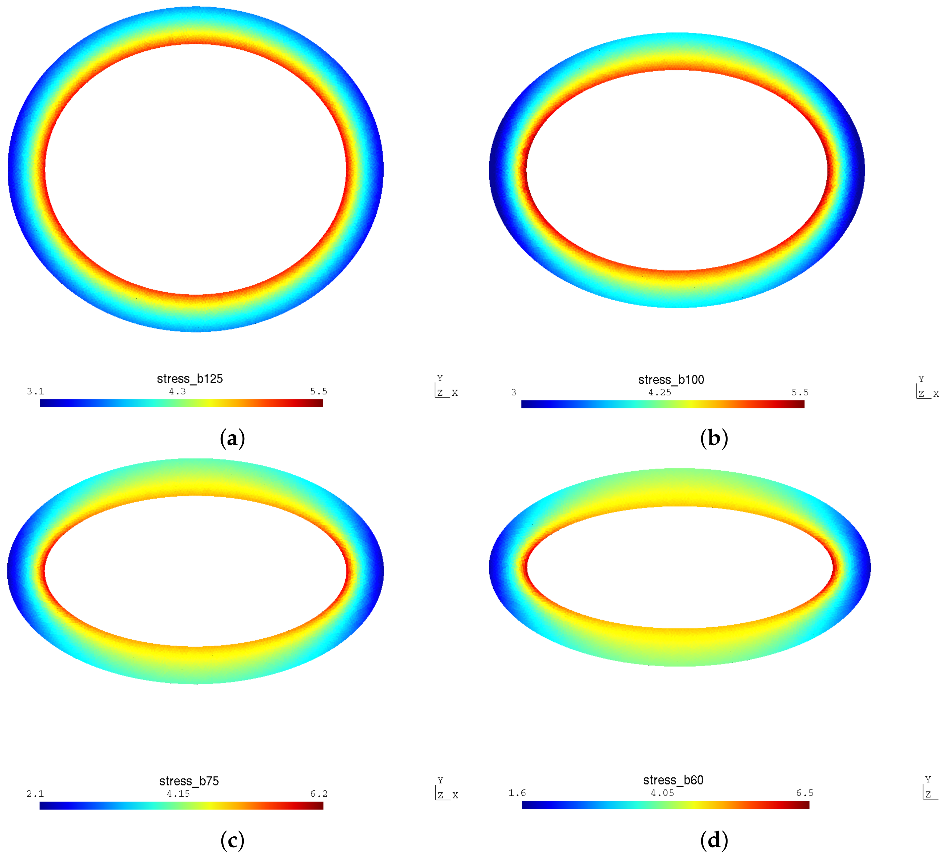
Figure 5 illustrates the von Mises stress contour of the different ring configurations ranging from slightly to extremely elliptical before any damage detection. Clearly the geometry (the only variable in this computation series) has a great impact on the stress distribution. When the ring is perfectly circular, the stress is axisymmetric, resulting in an equal opportunity of crack initiation along the circumference. The more elliptical the ring gets, the more the stress field loses its symmetry (with respect to the origin). This suggests that if any damage or cracks are detected, the zone of interest will grow smaller as the ratio $\frac{a}{b}$ increases and will be more and more located near the major axis a. One could imagine that when b tends towards zero, the ring will be completely flattened with singularities located where the major axis is supposed to be. It is only natural that the position of any detected damage or crack will converge toward this singularity.

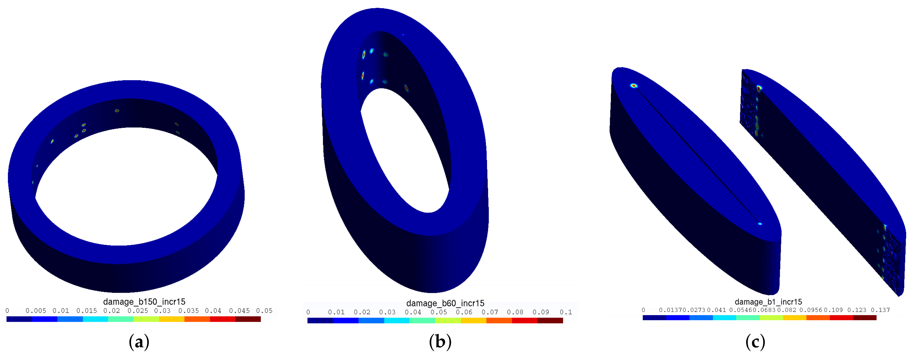
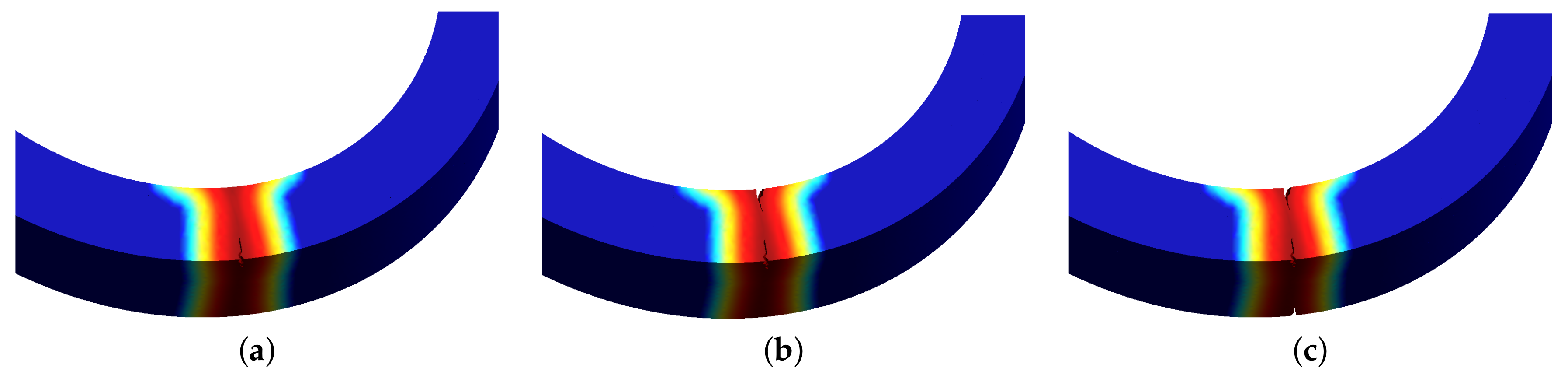
To reinforce this reasoning, the study is completed by a test case with $b=1$ mm ($\frac{a}{b}=150$) and is considered as the borderline case. Figure 6 illustrates the different damage zones detected after 15 increments for $\frac{a}{b}\in \{1,2.5,150\}$. Note that the damage d did not reach one yet. In other words, the results show the state of the rings before any crack initiation. Notice that, as expected, the different damaged zones are almost equi-distributed for the perfectly circular ring (Figure 6a) due to the equal opportunity of damage and crack initiation. As the ratio $\frac{a}{b}$ increases, the damaged zones are more and more located in the major axis vicinity (Figure 6b), and their position converges towards the singularity when $\frac{a}{b}\to \infty$ (Figure 6c).

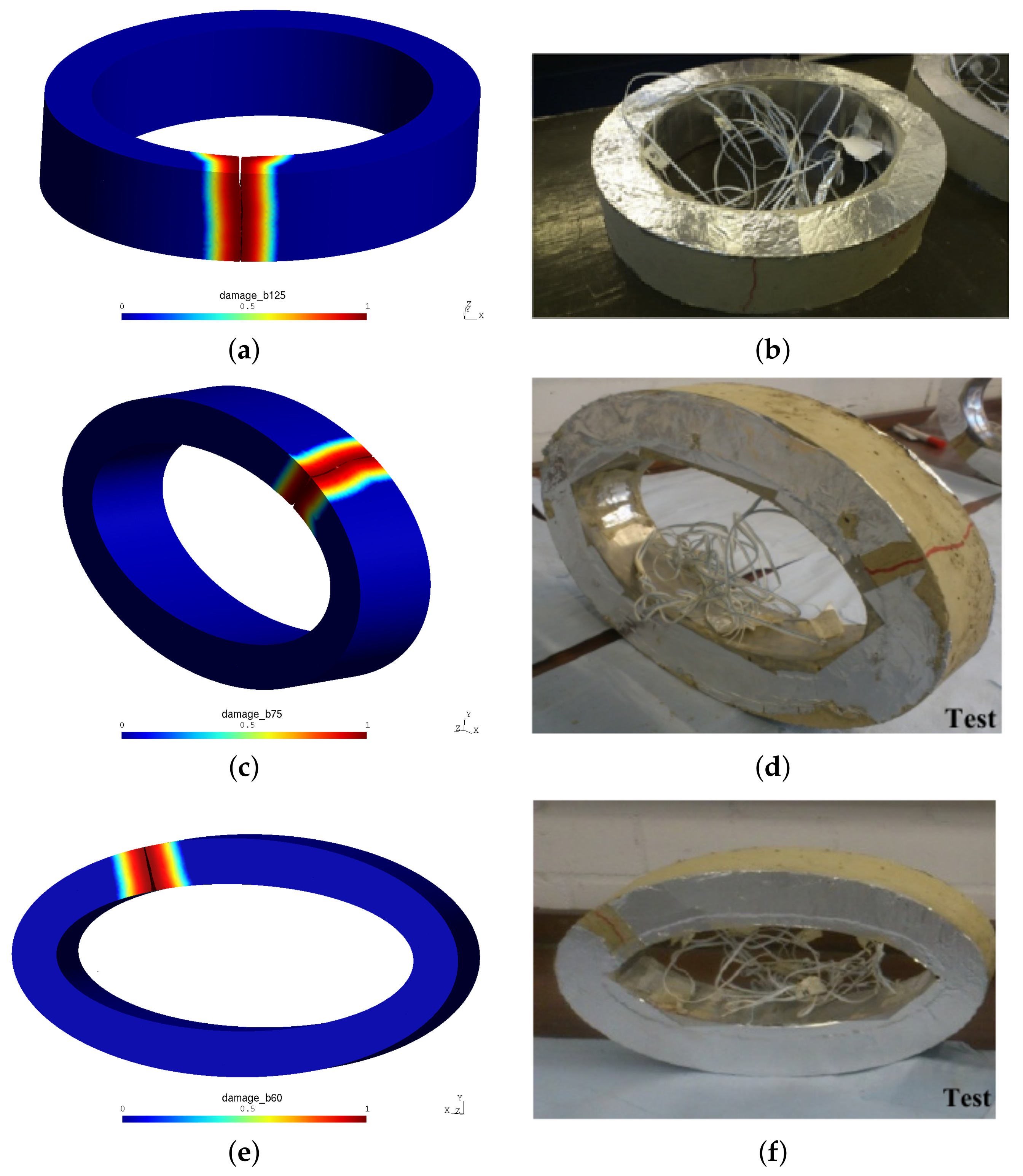
In addition, a comparison between the numerical results issued from the TLS model and the experimental ones collected from [17,27] is presented in Figure 7. The latter comparison not only shows a good agreement between the numerical and experimental campaigns, but also confirms that both damage and crack positions are affected by the oblateness severity. For the slightly elliptical ring ($\frac{a}{b}=1.2$), one crack passing through the wall thickness is visible lightly close to the minor axis (Figure 7a,b). As b decreases, the position of the crack moves closer towards the major axis (Figure 7c,e).

As mentioned earlier, the current version of the TLS model adopts a time-independent evolution law. In other words, the algorithm is governed by damage front advance rather than a time-step control. This is why the exact day on which a crack first appears cannot be determined automatically.

Nevertheless, it is still possible to determine a relationship between the ratio $\frac{a}{b}$ and the needed shrinkage to initiate a damage. Additional post-processing is needed to retrieve the response pattern of the TLS model. For the sake of clarity, the post-processing is explained on the circular ring case ($\frac{a}{b}=1$) in Figure 8 before presenting the results for the whole range of test cases.

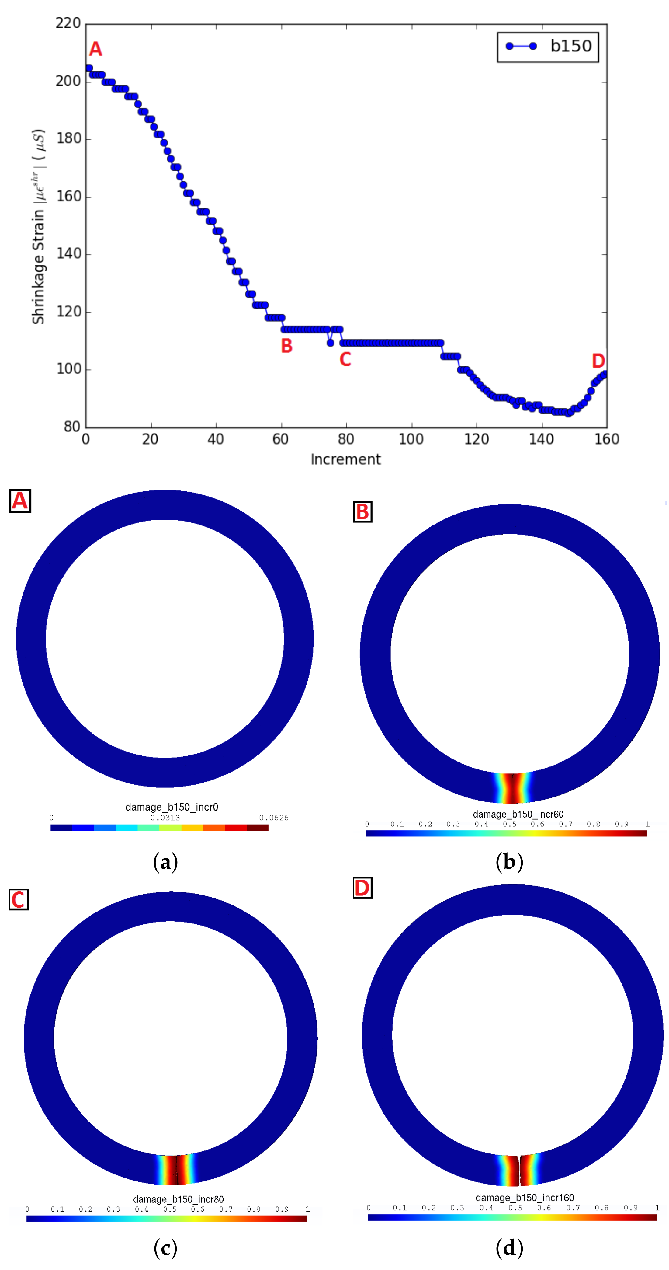
The evolution of the load factor $|\mu {\epsilon }^{shr}|$ as a function of the simulation increments is plotted. The ring state is presented for four different points, denoted A, B, C and D on the curve, respectively in Figure 8a–d. Point A corresponds to the first damage introduced for a load factor ${\mu }_0=209.94$ (i.e., shrinkage strain equal to $-209.94\frac{\mu \mathrm{m}}{\mathrm{m}}$). Point B corresponds to the increment for which the damage reaches one and a crack is initiated for the first time. Point C corresponds to the increment for which the crack propagated completely on the top side of the ring. Finally, Point D corresponds to the increment for which the crack goes through the whole thickness and wall, breaking the ring altogether.

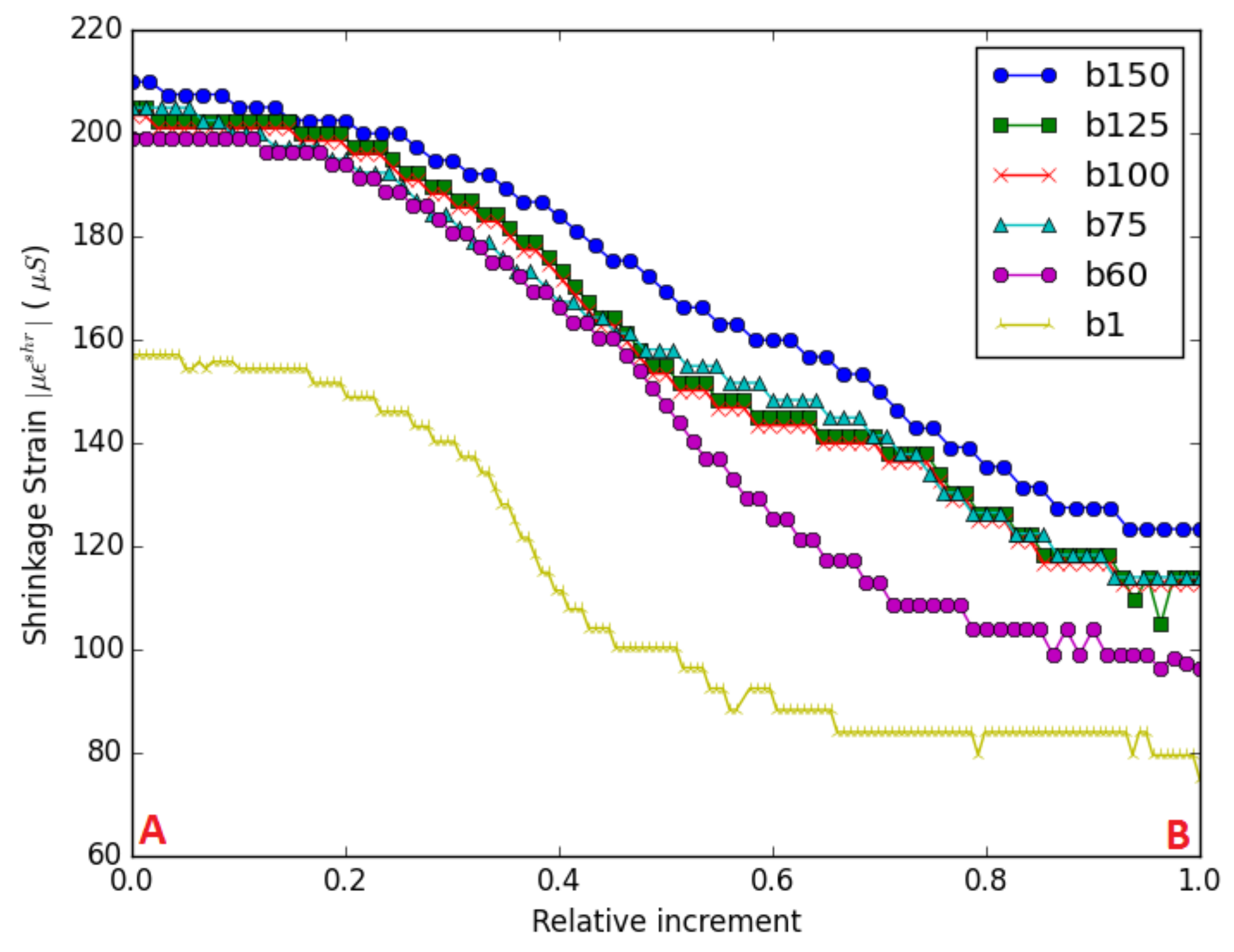
To superpose the curves for the different test cases and due to the lack of time notion, the increment for which the crack is first initiated (i.e., Point B) is manually determined for each case and is called $inc{r}_{a/b}^{d=1}$. The latter is equal to 60 for the circular ring. Relative increments are then determined as $\frac{incr}{inc{r}_{a/b}^{d=1}}$, and all curves are consequently plotted on $[0,1]$ (i.e., between Points A and B) in Figure 9.

All curves are bound between two limits, the upper one for $\frac{a}{b}=1.$ and a lower one for $\frac{a}{b}\to \infty$. Increasing the ratio $\frac{a}{b}$ yields smaller critical shrinkage loads capable of initiating a damage (i.e., Point A), then a crack (i.e., Point B). The overall behavior is consistent and promising.

We focus next on determining some kind of time interval for when the damage first appears.

Table 2. Shrinkage strain for different $\frac{a}{b}$ ratios; ${\mu }_0$ denotes the loading factor computed to introduce an initial damage.

$\frac{\mathit{a}}{\mathit{b}}$	1	1.2	1.5	2	2.5	3.75	150
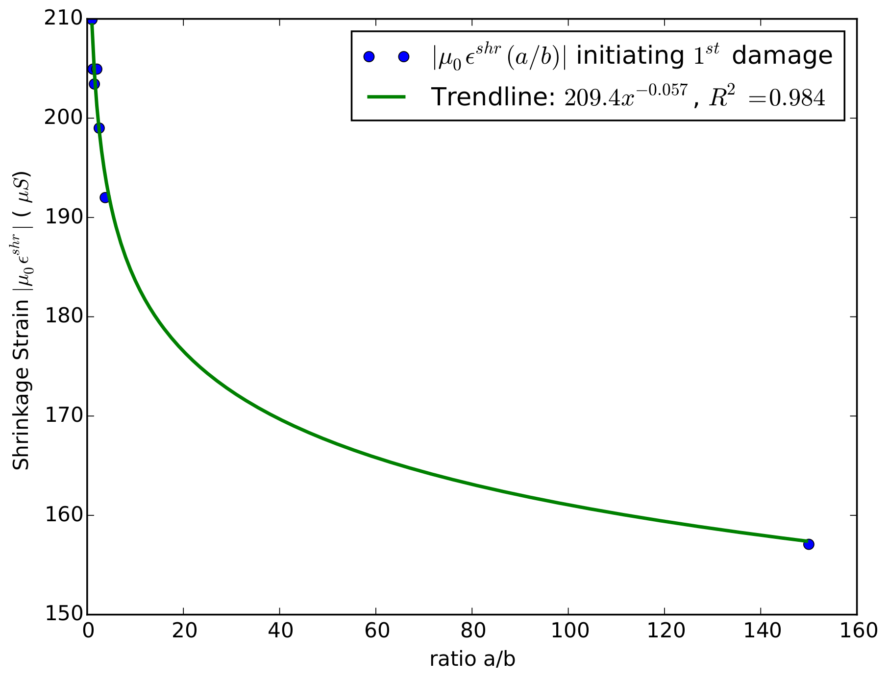
$|{\mu }_0{\epsilon }^{shr}|\left(\mu S\right)$	209.94	205	203.44	204.94	199	192	157.1

and Figure 10 summarize the different shrinkage values $|{\mu }_0{\epsilon }^{shr}|$ for which an initial partial damage (not yet a visible macroscopic crack) is initiated (i.e., Point A). The higher the oblateness a ring has, the less shrinkage it tolerates before a damage appears. The trend line fit of $\left(\right|{\mu }_0{\epsilon }^{shr}{\left|\right)}_{a/b\in [1,150]}$ shows that the needed shrinkage to introduce damage is a decreasing function of $\frac{a}{b}$ with a decreasing rate.

The authors of [17,27] determined that “Cracking ages of the circular ring and elliptical rings with $\frac{a}{b}<2$, i.e., in this case $b=125$ or 100 mm, are all close to 15 days. However, elliptical rings with $\frac{a}{b}\ge 2$, i.e., in this case $b=75$ or 60 mm, cracked much earlier at around 11 and 13 days, respectively, on average”. Aiming to determine a time interval, values summarized in Table 2 are placed on the free shrinkage experimental measurements obtained by [17,27]. 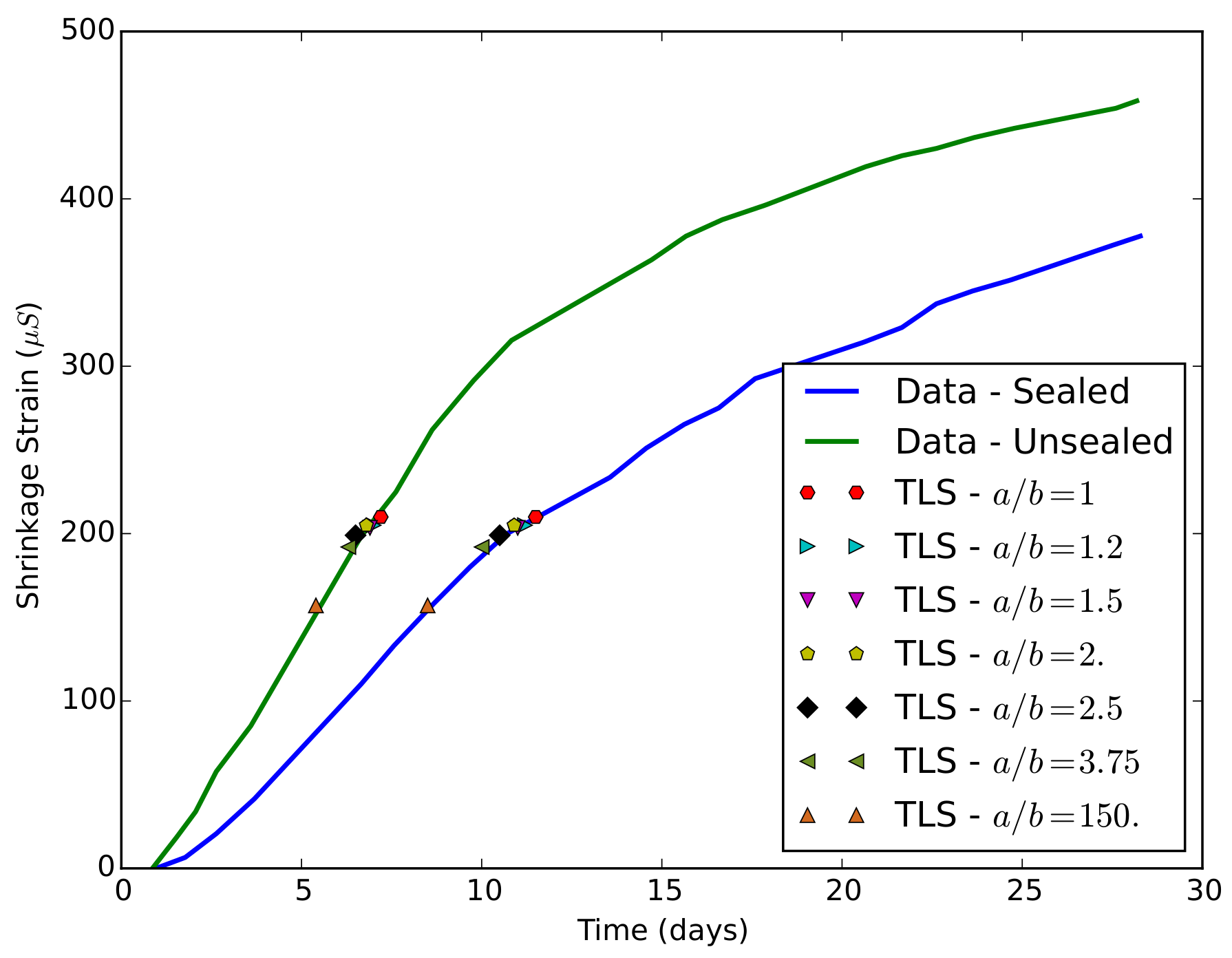Figure 11 illustrates two different scenarios where numerical shrinkage values $|{\mu }_0{\epsilon }^{shr}|$ are linked to free shrinkage data for respectively sealed and unsealed specimens.

If linked with the experimental curve under sealing conditions, the damage first starts around Day 12 for the circular and slightly elliptical rings (i.e., $\frac{a}{b}<2$) and around Day 10 for more elliptical rings (i.e., $\frac{a}{b}\ge 2$).

If linked with the experimental curve without sealing conditions, the damage first starts around Day 7 for the circular and slightly elliptical rings (i.e., $\frac{a}{b}<2$) and around Day 6 for more elliptical rings (i.e., $\frac{a}{b}\ge 2$). Earlier damage initiation is expected if no sealing conditions are applied due to the bigger exposed surface to drying.

Overall, the damage initiation times (not yet visible cracks) are consistent. The damage appears earlier with an increasing oblateness due to a higher degree of auto-restraint provided by the ring itself. In addition, the determined damage times are compatible with the cracking times observed by [17,27].

4. Discussion

In this work, a first attempt using the novel TLS model for shrinkage-induced cracking in concrete applications is presented. Shrinkage contribution was taken into account in a simple, yet efficient manner. The overall behavior of the model is tested. Despite the simplicity considered herein, the first results are promising.

(i)

Rings’ oblateness induces a higher degree of auto-restraint and therefore has a great impact on stress distribution, damage zone initiation and crack positions:

• Increasing the ratio $a/b$ and the ellipticity of the rings showed that stress concentration (i.e., critical zones) is more and more located near the major axis. Different damaged zones were consequently detected and initiated.
• A comparison between critical shrinkage strains needed to initiate damage and eventually cracks proved to be dependent on the oblateness severity. Less shrinkage is needed to initiate damage for highly elliptical rings suggesting that damage and cracking times are shorter for elliptical rings.

(ii)

The crack position and trajectory matches the experimental observations presented in [17,27]. A single crack going through the ring wall was detected.

The TLS model offers a more complete insight in particular into the transition between damage and fracture. Contrary to other numerical models and experimental tests, the damage evolution is tracked, and crack initiation is observed when damage reaches exactly one. For illustration purposes, let us take the case using $\frac{a}{b}=1.2$. Figure 12 presents the state of the ring at different increments just after initial cracking.

Notice that a small crack appears on the top outer side of the ring in Figure 12a, followed by similar ones on the inner upper and outer bottom sides of the ring, respectively illustrated in Figure 12a,b. The cracks grow closer and then merge to form one single crack going through the ring wall (see Figure 7a). This information is very important for industrial cases where the position of the initial crack and the interaction between neighbor cracks is crucial.

To summarize, the numerical results are encouraging and agree fairly well with the experimental findings. The capacity of the TLS model was tested and judged solid.

Moving forward, there is plenty of room for improvements. The model can be enhanced by introducing:

(i)

Richer shrinkage strain fields instead of the mean values averaged on a cross-section:

Taking the mean shrinkage value as adopted in this work as the main actor for crack initiation cannot be generalized for complex geometries, with different cross-sections or for special conditions affecting the homogeneity of the drying process such as sealing or curing. Bažant in [30] proposes to treat concrete drying as a nonlinear diffusion equation expressing Fick’s law to govern the loss of moisture. Afterward, several studies followed the same logic. We cite for instance the work presented in [31] where chaining two computations is recommended; a thermal computation followed by a drying one. Shrinkage is no longer a mean value homogeneously represented all over the domain, but rather a heterogeneous field taking into account thermal and drying boundary conditions.

(ii)

Time-dependent material properties or at least evolving properties with the simulation progress: Early age concrete properties such as the Young’s modulus and tensile strength are increasing functions of time (for $t\le 28$ days).

(iii)

A time-controlled evolution algorithm enabling the model to correlate damage and crack initiation to an exact and well-known time.