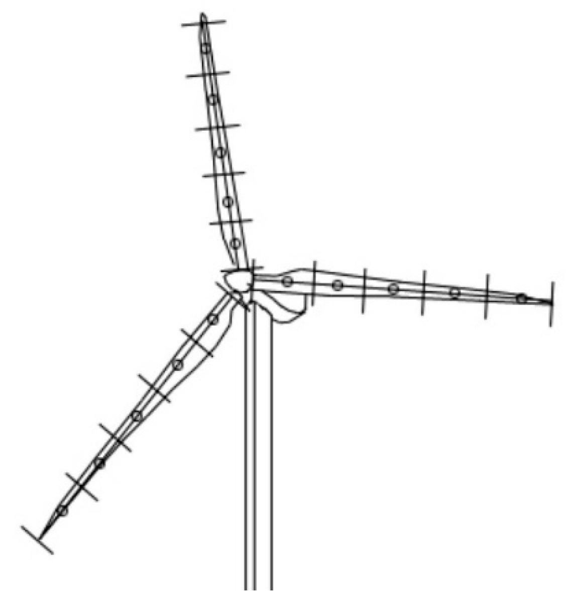
Figure 1.
Blades represented by actuator lines.
Figure 1.
Blades represented by actuator lines.
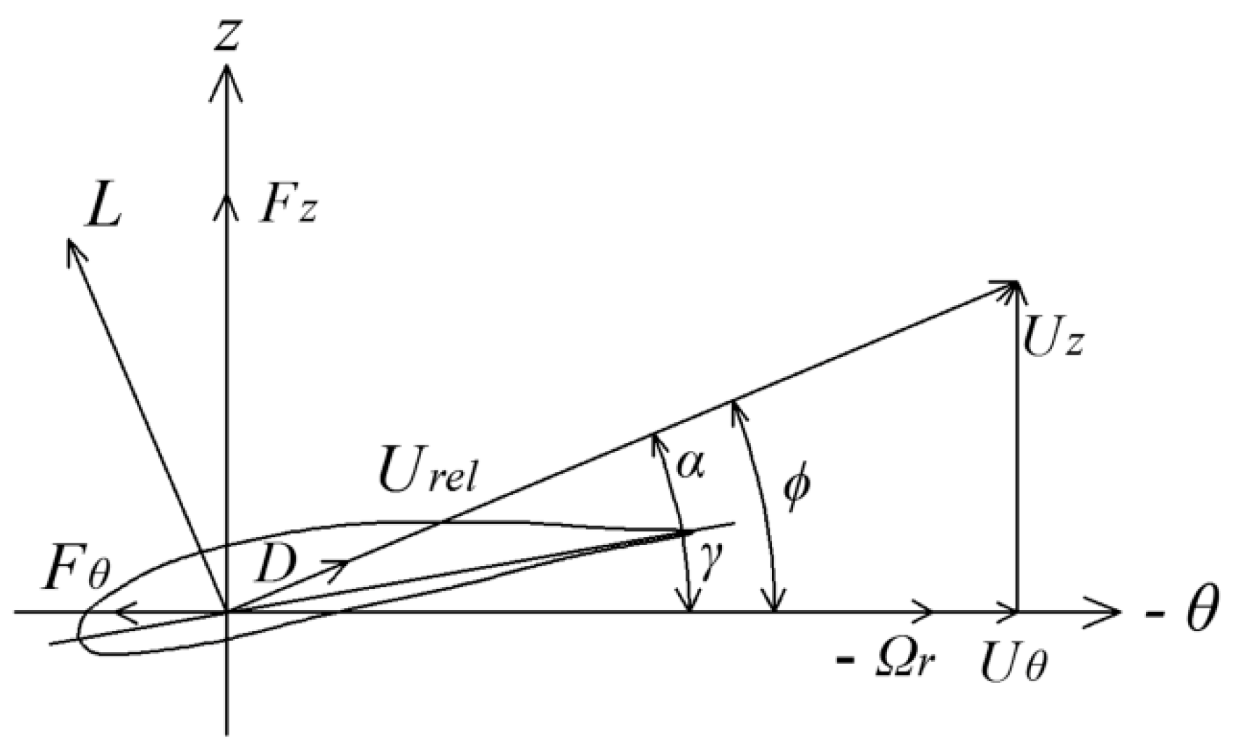
Figure 2.
Cross-sectional airfoil element.
Figure 2.
Cross-sectional airfoil element.
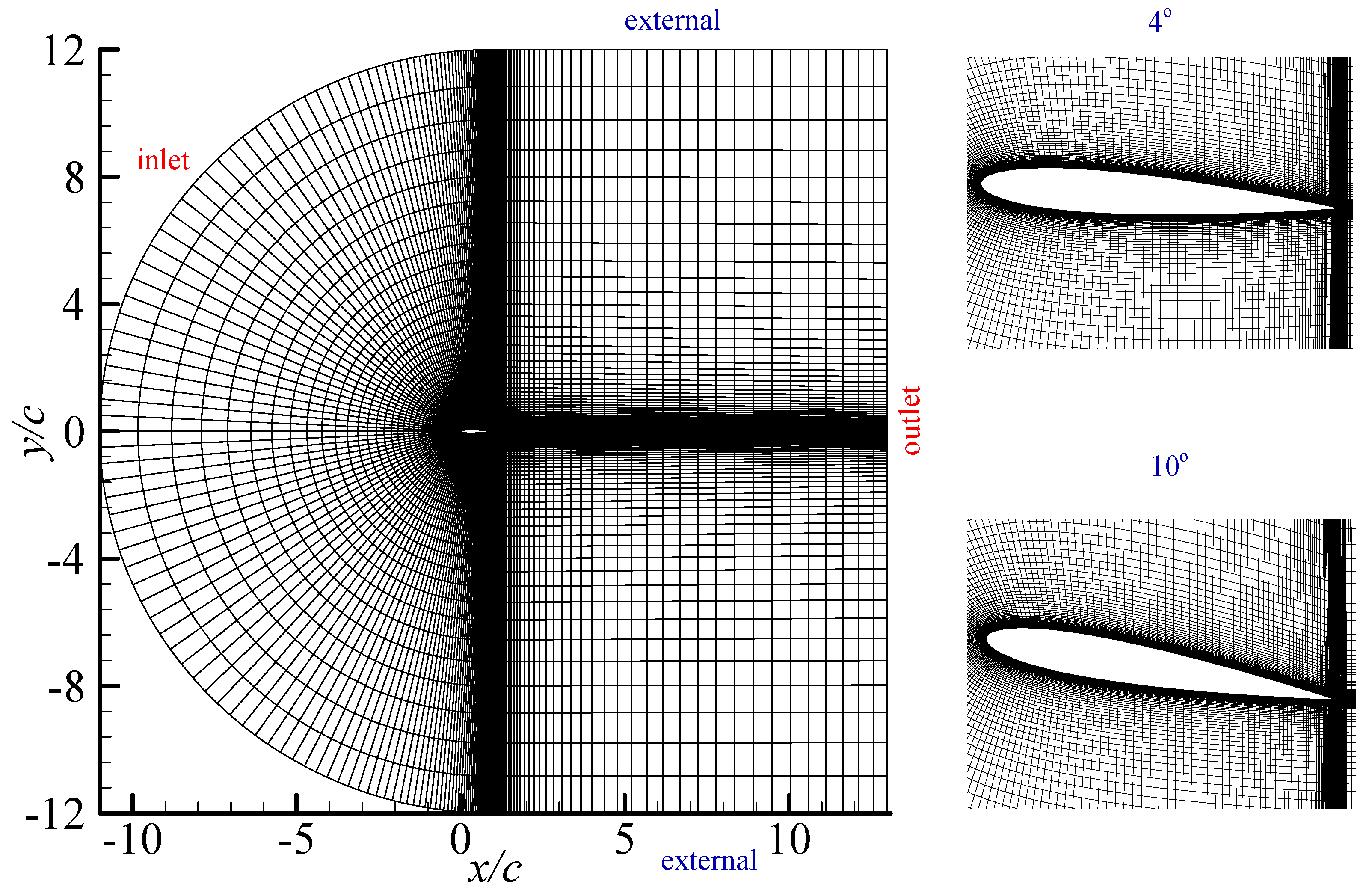
Figure 3.
Simulation domain of NACA0012. NACA: National Advisory Committee for Aeronautics.
Figure 3.
Simulation domain of NACA0012. NACA: National Advisory Committee for Aeronautics.
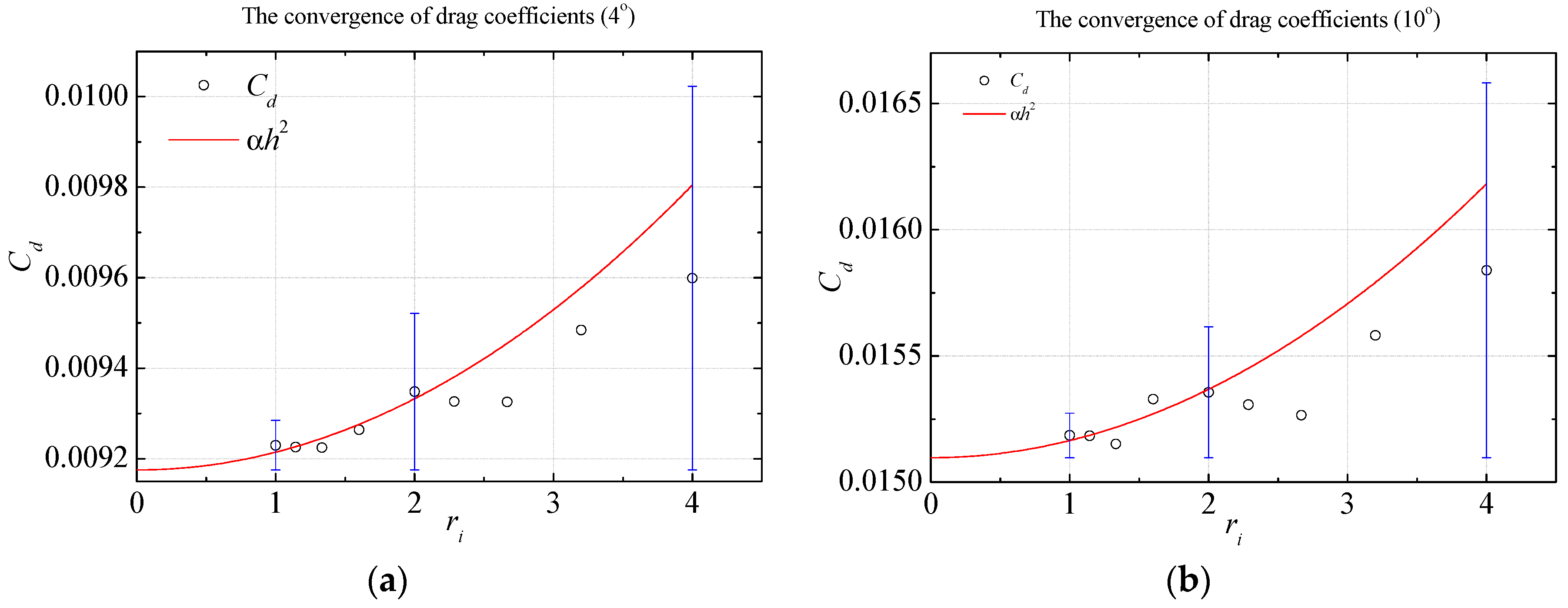
Figure 4.
Convergence of the drag coefficient with the grid refinement (Fits obtained from the data with ) by different attack angles: (a) 4°; (b) 10°. Blue line: Error bar.
Figure 4.
Convergence of the drag coefficient with the grid refinement (Fits obtained from the data with ) by different attack angles: (a) 4°; (b) 10°. Blue line: Error bar.
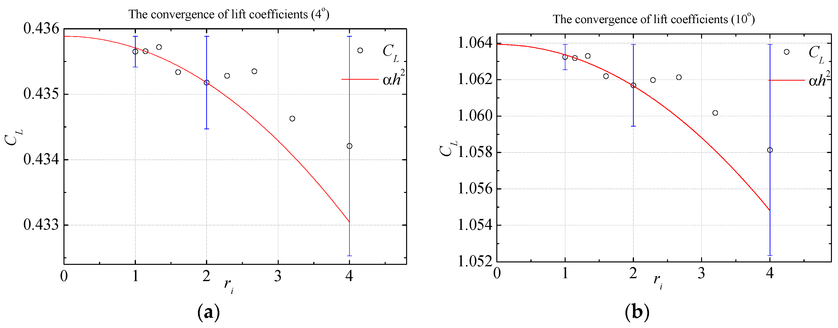
Figure 5.
Convergence of the lift coefficient with the grid refinement (Fits obtained from the data with ) by different attack angles: (a) 4°; (b) 10°. Blue line: Error bar.
Figure 5.
Convergence of the lift coefficient with the grid refinement (Fits obtained from the data with ) by different attack angles: (a) 4°; (b) 10°. Blue line: Error bar.
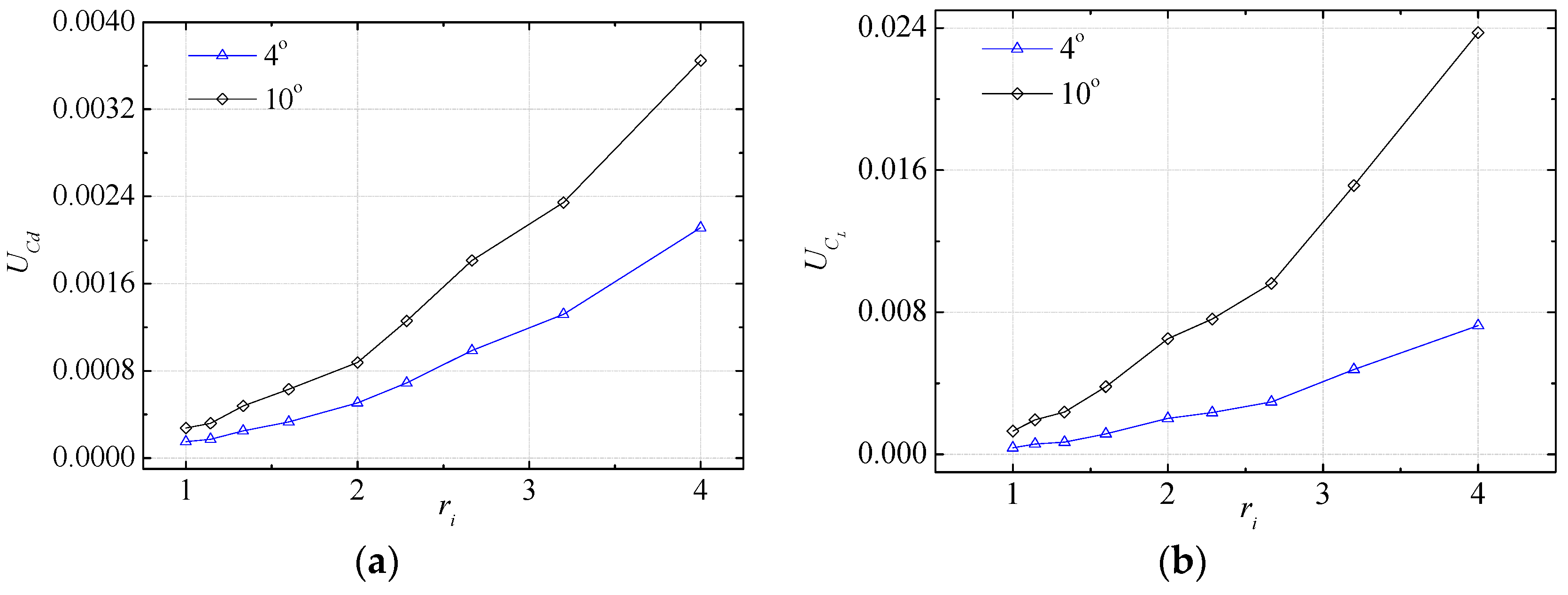
Figure 6.
Uncertainty of the drag and lift coefficient with the grid refinement for different attack angles: (a) UCL; (b) UCd.
Figure 6.
Uncertainty of the drag and lift coefficient with the grid refinement for different attack angles: (a) UCL; (b) UCd.
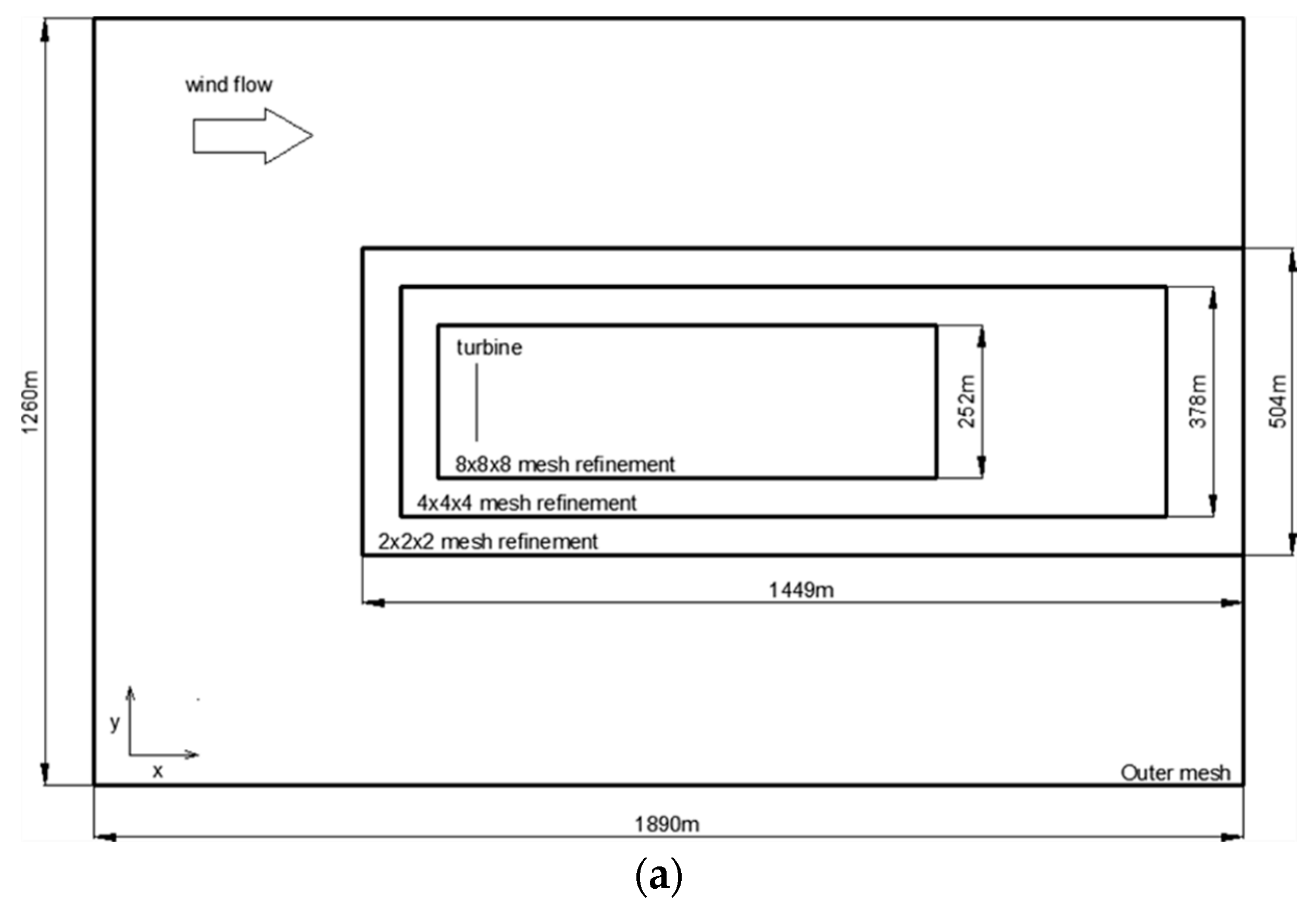
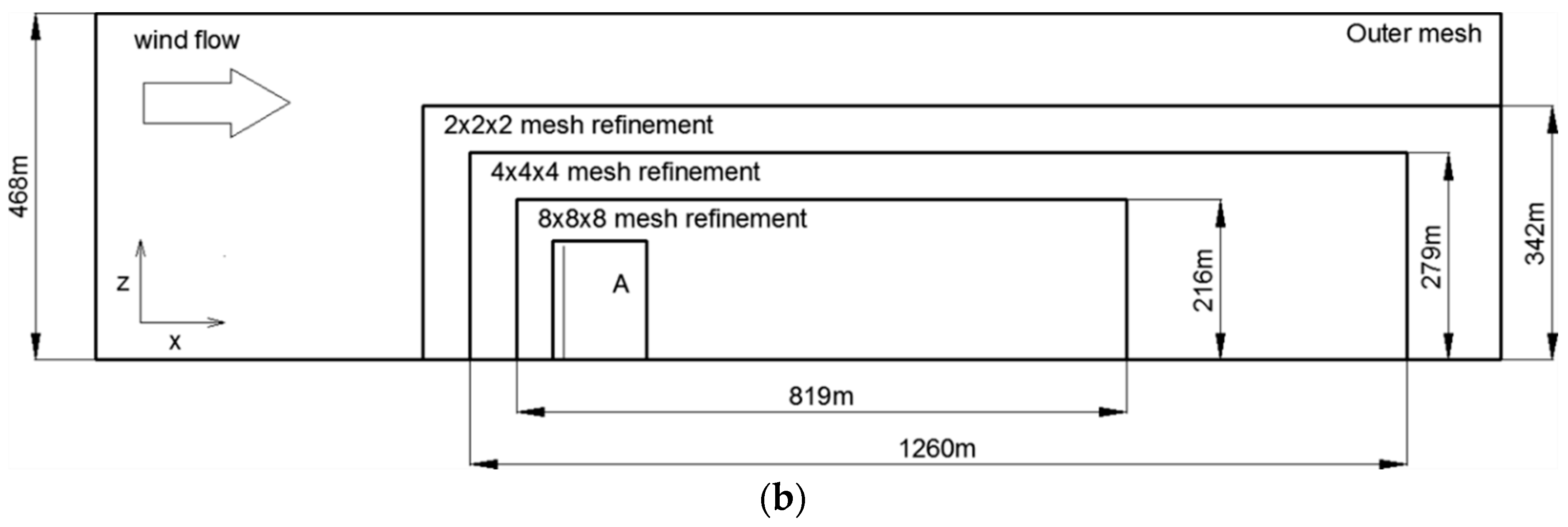
Figure 7.
The schematic setup of computational domain: (a) Top view; (b) Side view.
Figure 7.
The schematic setup of computational domain: (a) Top view; (b) Side view.
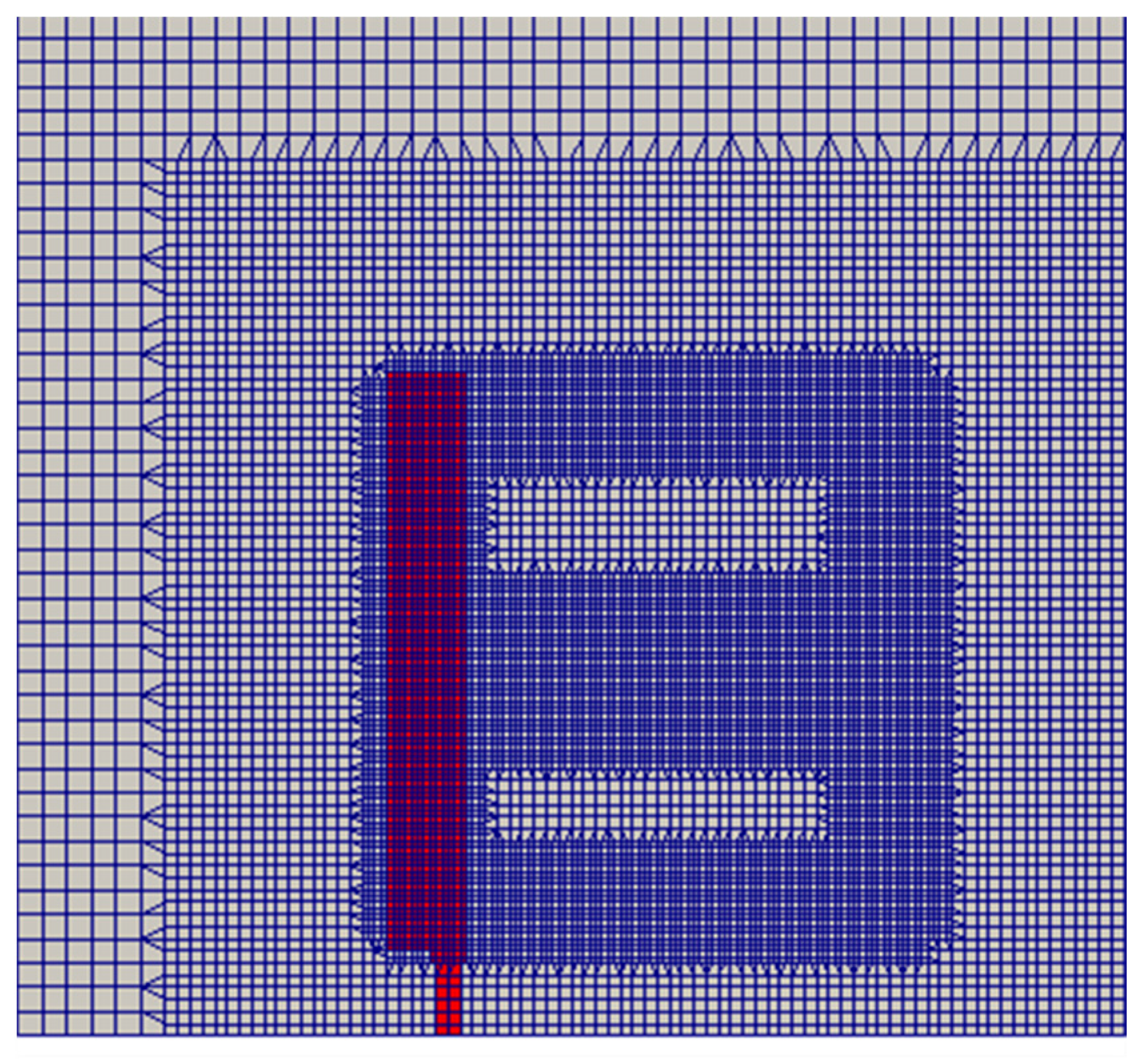
Figure 8.
Computational domain mesh of A with refinement. The blue mesh is the fluid domain; the red mesh is the part of wind turbine.
Figure 8.
Computational domain mesh of A with refinement. The blue mesh is the fluid domain; the red mesh is the part of wind turbine.
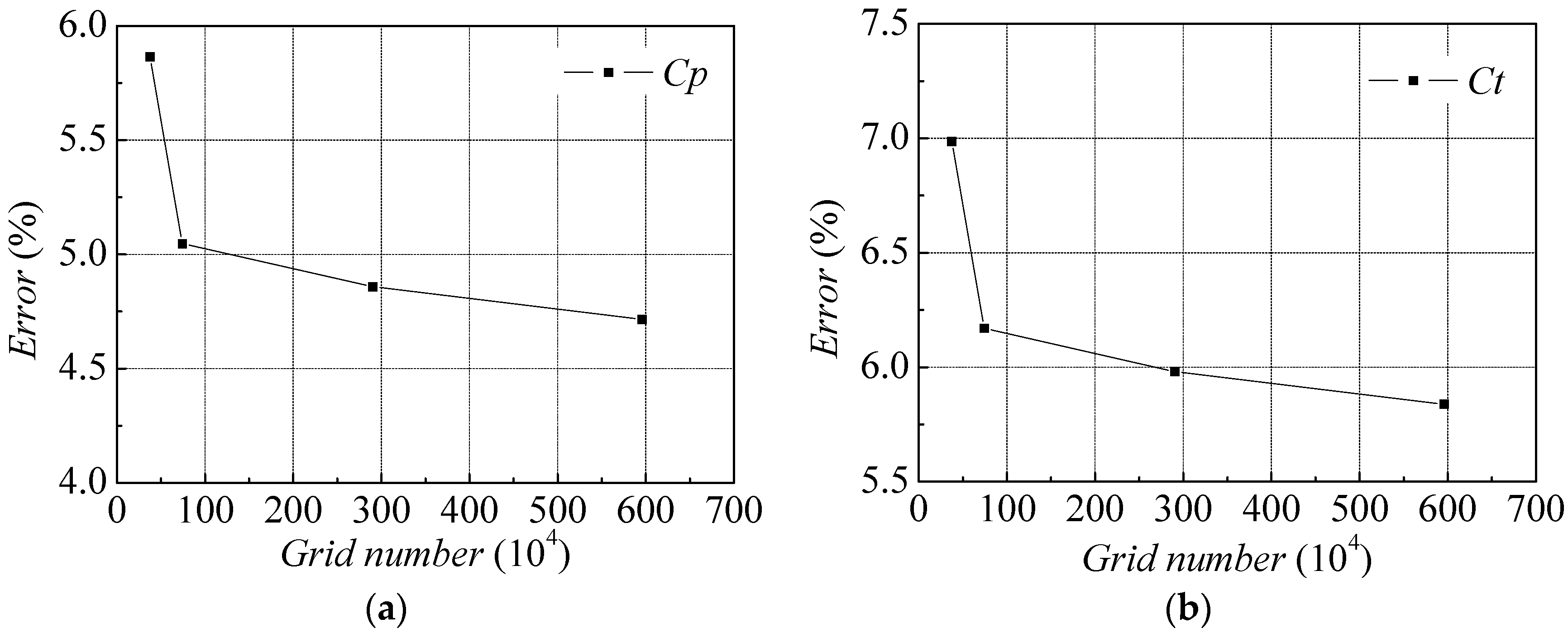
Figure 9.
The mesh independence test: (a) Error distributions of Cp; (b) Error distributions of Ct.
Figure 9.
The mesh independence test: (a) Error distributions of Cp; (b) Error distributions of Ct.
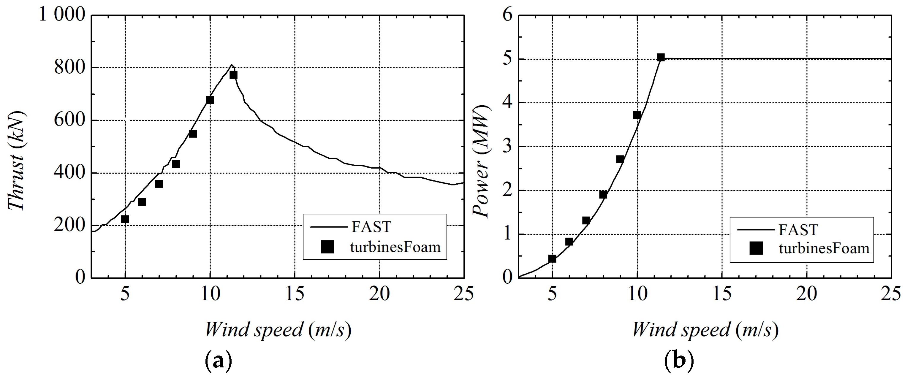
Figure 10.
Comparison of the computed power and thrust between FAST and turbinesFoam at different wind speed: (a) Thrust; (b) Power.
Figure 10.
Comparison of the computed power and thrust between FAST and turbinesFoam at different wind speed: (a) Thrust; (b) Power.
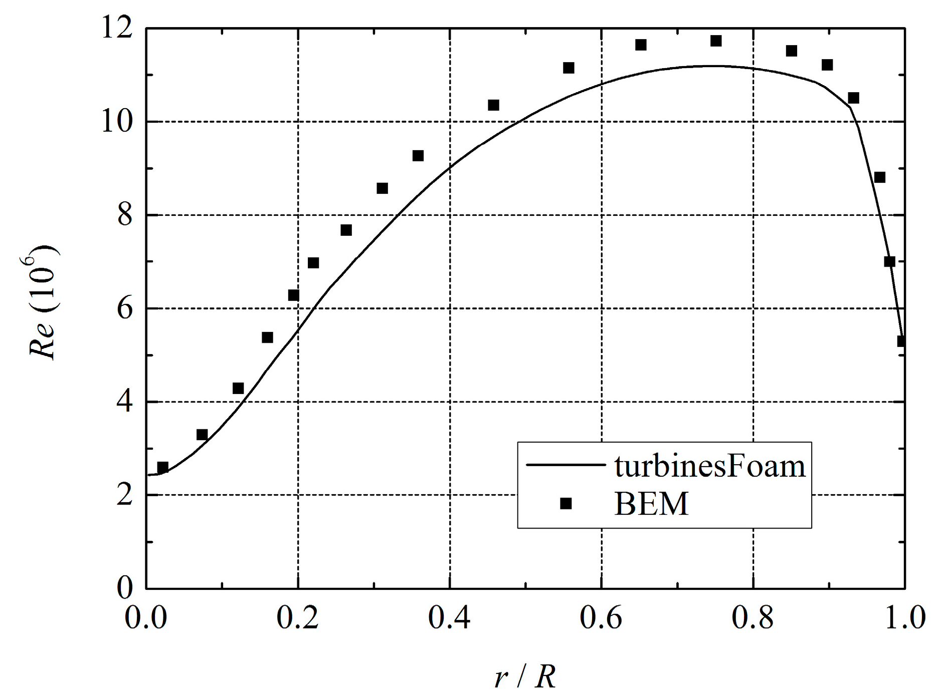
Figure 11.
Comparison of the local Reynolds number with the Blade-Element/Momentum (BEM) method.
Figure 11.
Comparison of the local Reynolds number with the Blade-Element/Momentum (BEM) method.
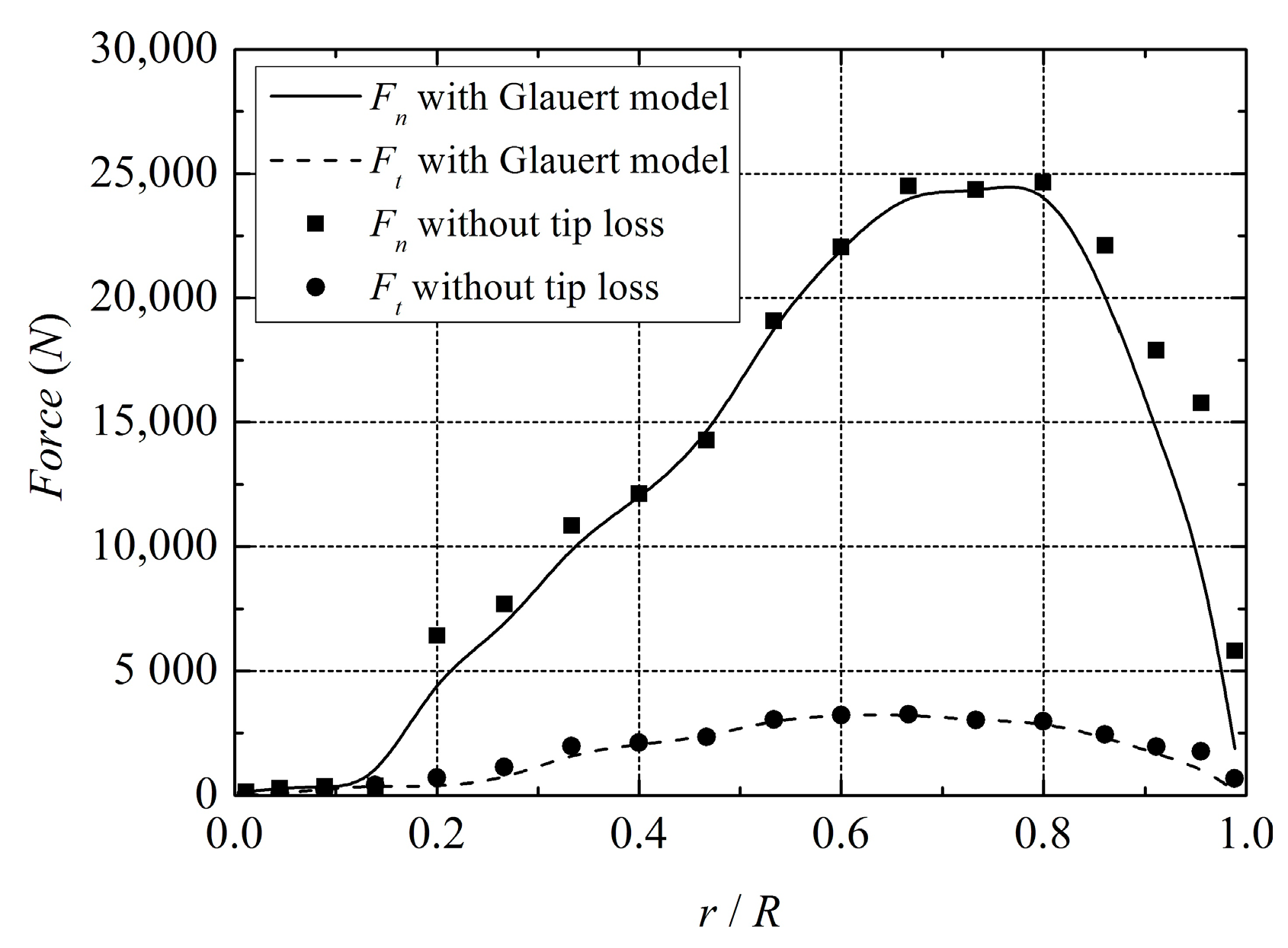
Figure 12.
Comparison of radial force distributions with Glauert model and without the tip loss model.
Figure 12.
Comparison of radial force distributions with Glauert model and without the tip loss model.
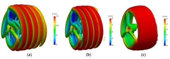
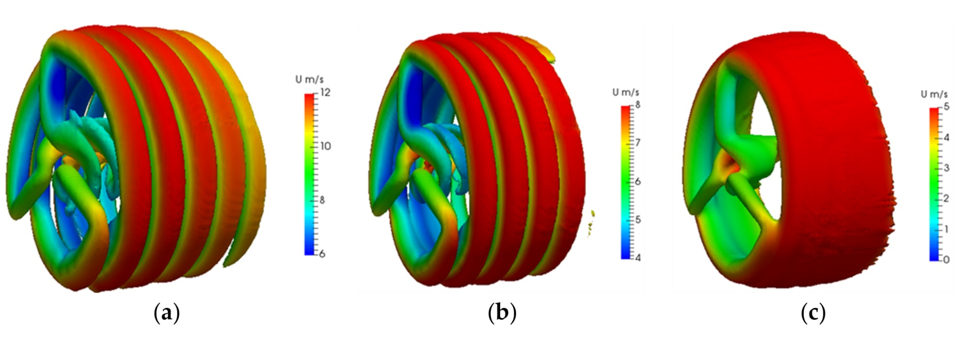
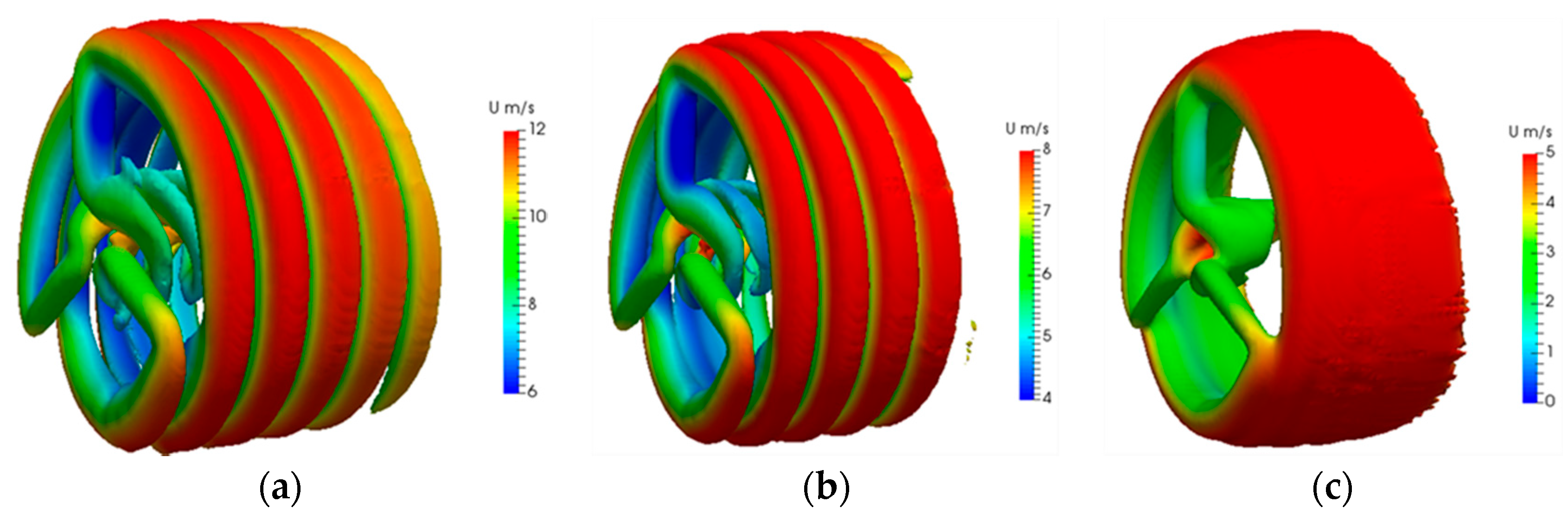
Figure 13.
Computed Q field showing the formation of wake structure (Q = 0.003): (a) U0 = 11.4 m/s; (b) U0 = 8 m/s; (c) U0 = 5 m/s.
Figure 13.
Computed Q field showing the formation of wake structure (Q = 0.003): (a) U0 = 11.4 m/s; (b) U0 = 8 m/s; (c) U0 = 5 m/s.
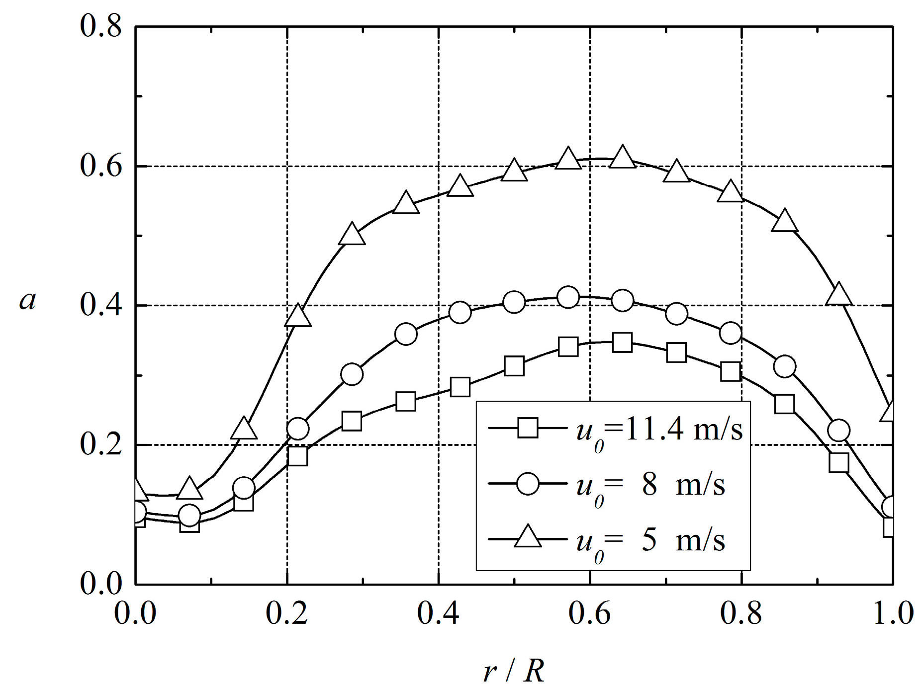
Figure 14.
Radial distributions of averaged axial flow interference factors at different wind speeds.
Figure 14.
Radial distributions of averaged axial flow interference factors at different wind speeds.
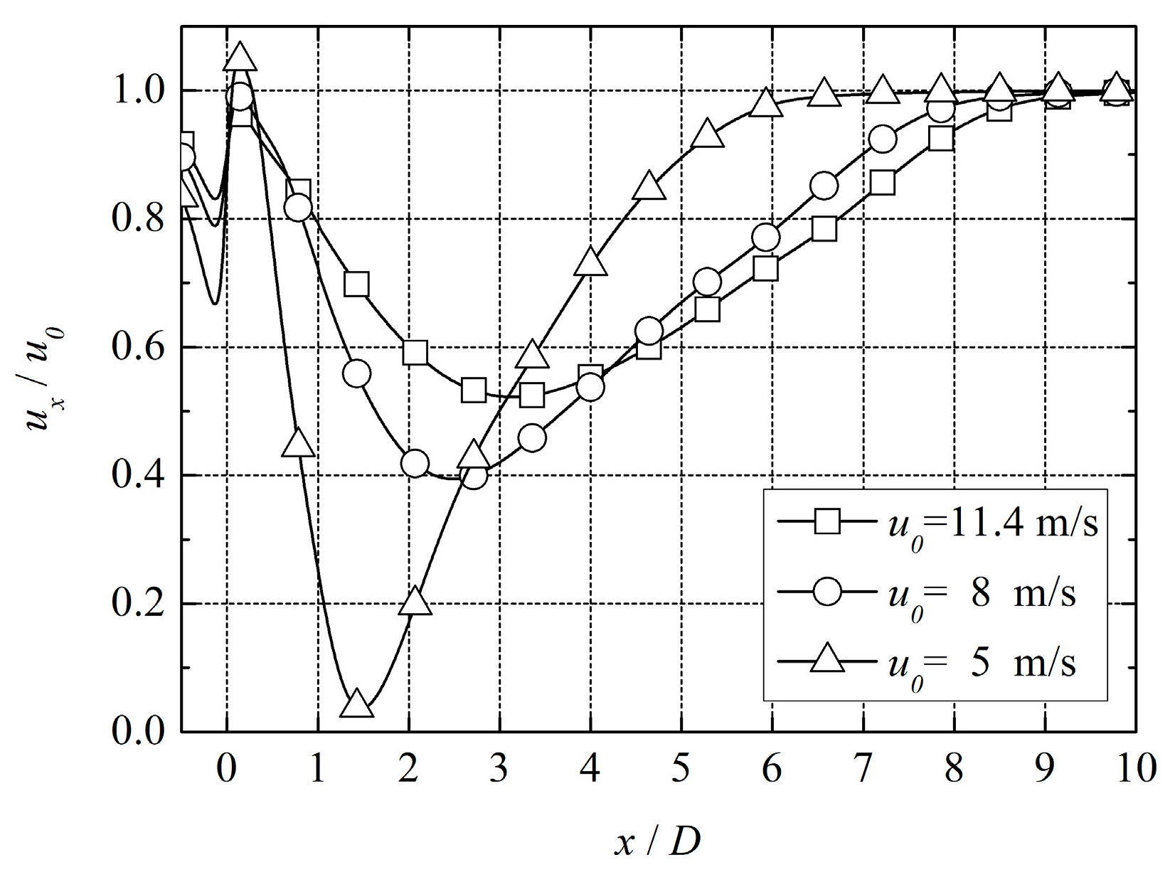
Figure 15.
Streamwise profile of the average axial velocity at hub height.
Figure 15.
Streamwise profile of the average axial velocity at hub height.
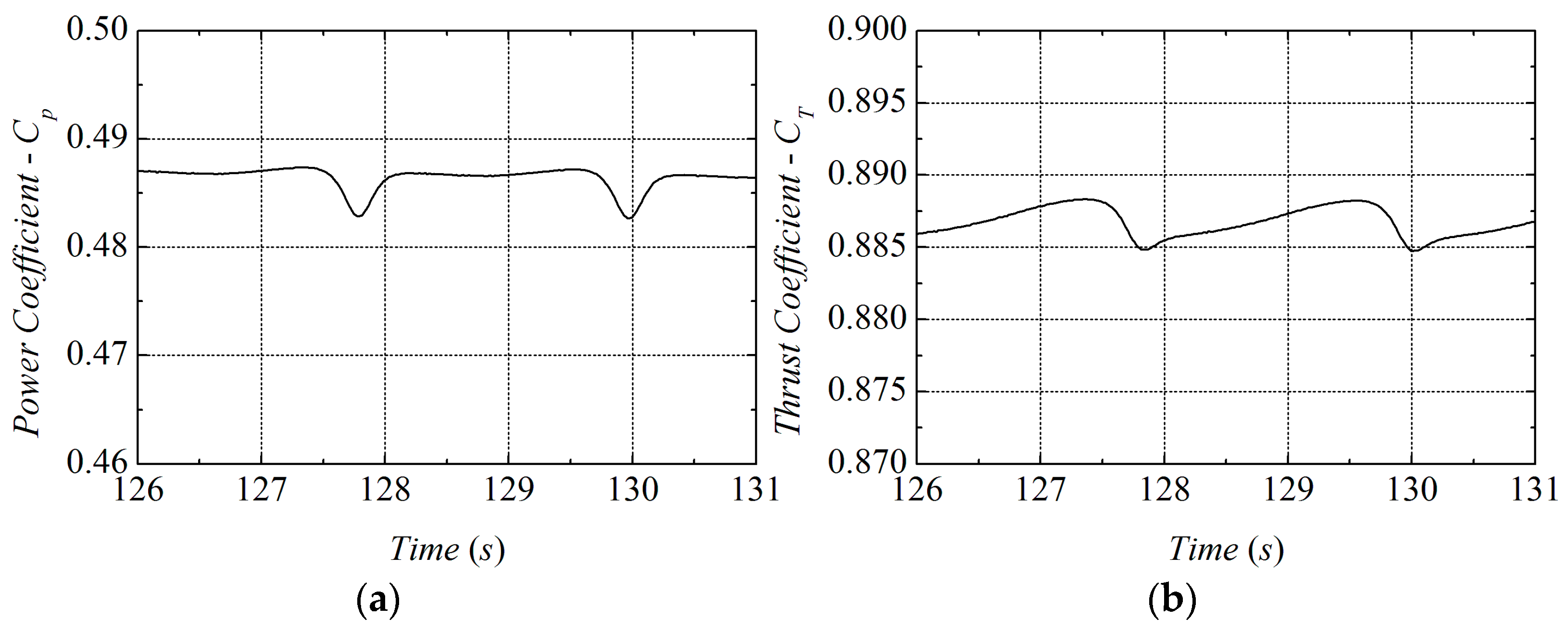
Figure 16.
The curves of power and thrust coefficient: (a) Power coefficient; (b) Thrust coefficient.
Figure 16.
The curves of power and thrust coefficient: (a) Power coefficient; (b) Thrust coefficient.
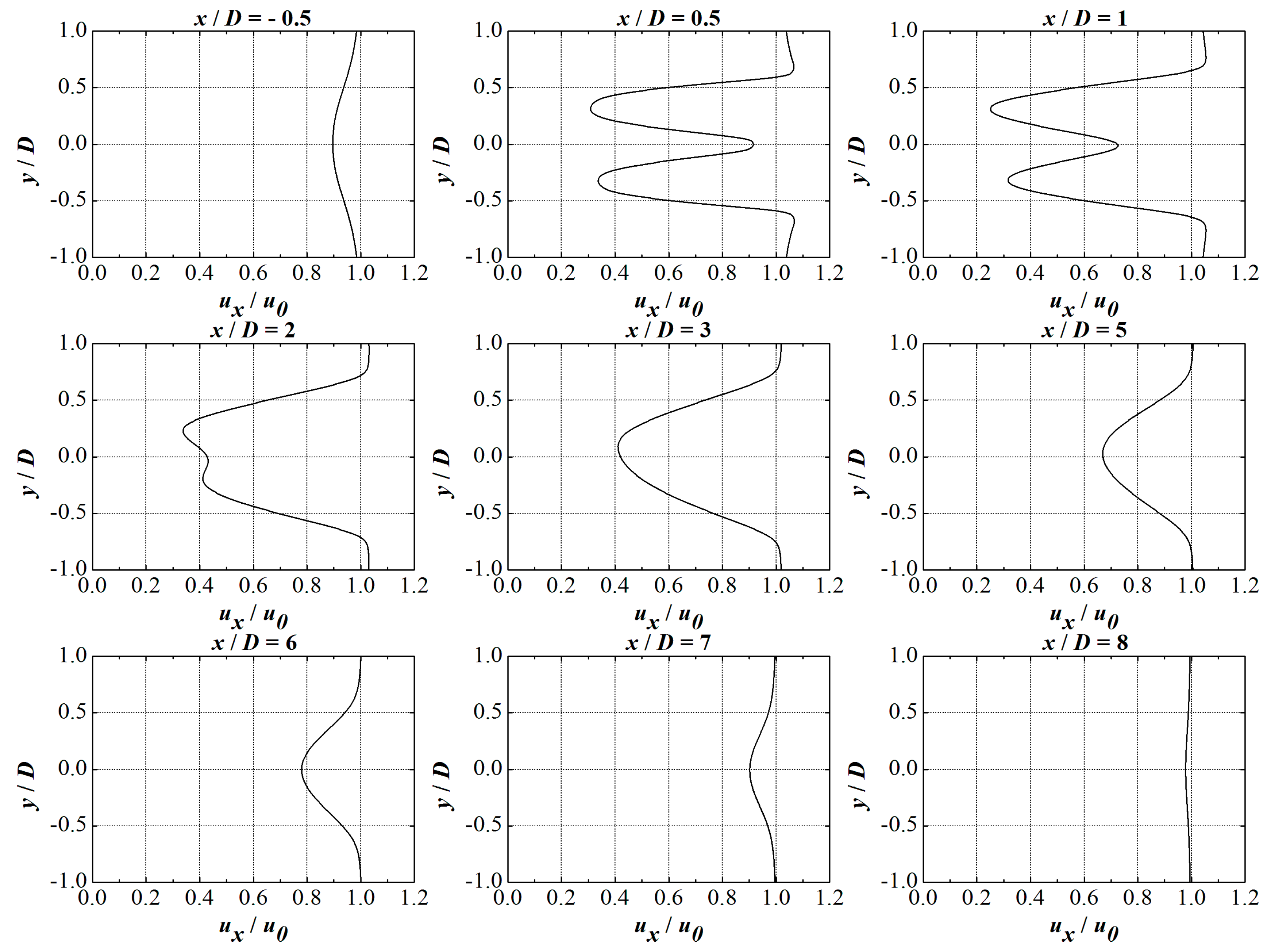
Figure 17.
Spanwise distribution of average axial velocity in different streamwise locations.
Figure 17.
Spanwise distribution of average axial velocity in different streamwise locations.
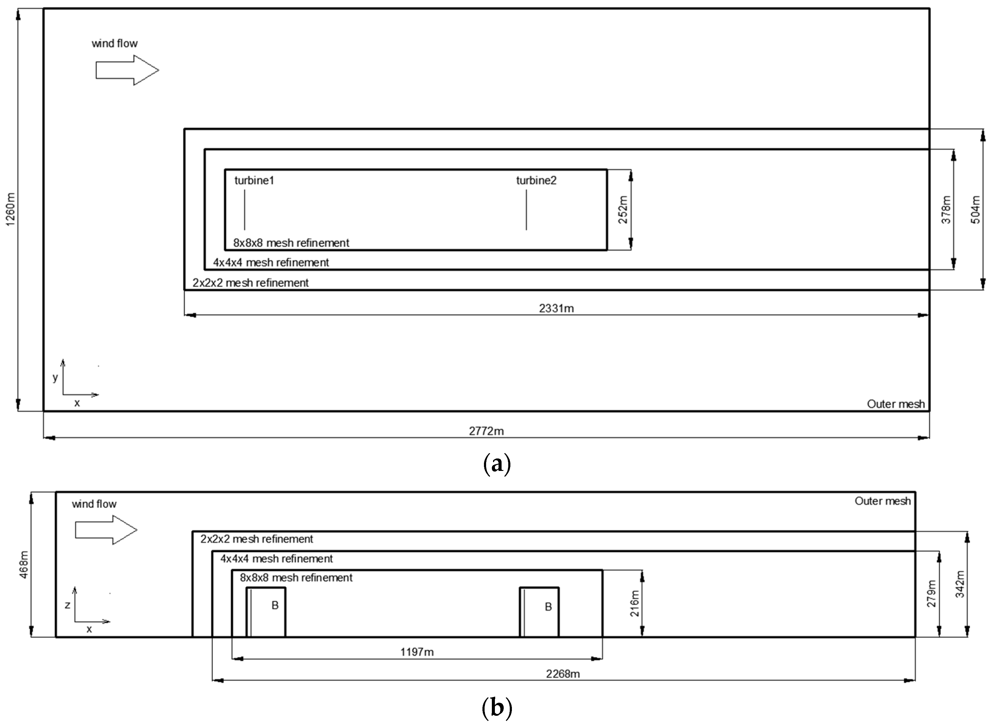
Figure 18.
Schematic setup of two wind turbines domain: (a) Top view; (b) Side view.
Figure 18.
Schematic setup of two wind turbines domain: (a) Top view; (b) Side view.
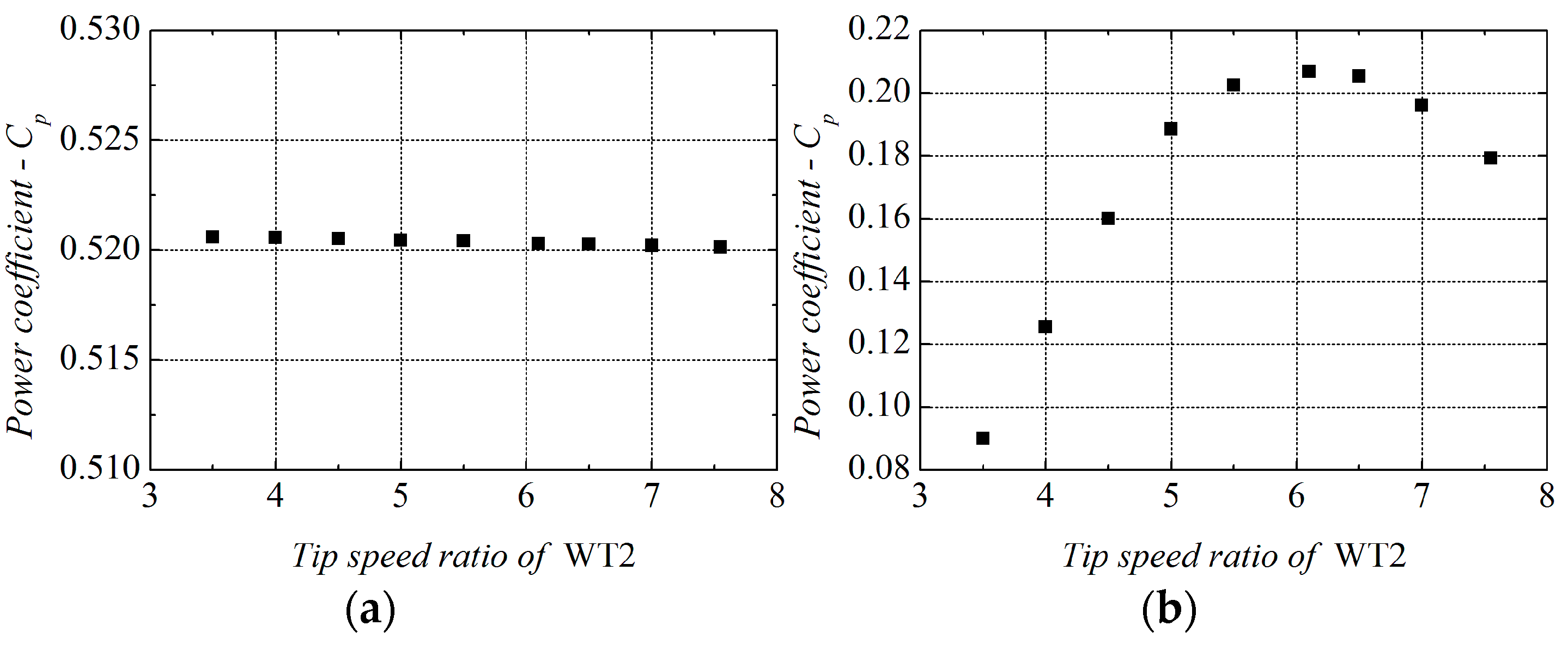
Figure 19.
Power coefficient with different tip speed ratio of WT2: (a) Power coefficient of WT1; (b) Power coefficient of WT2.
Figure 19.
Power coefficient with different tip speed ratio of WT2: (a) Power coefficient of WT1; (b) Power coefficient of WT2.
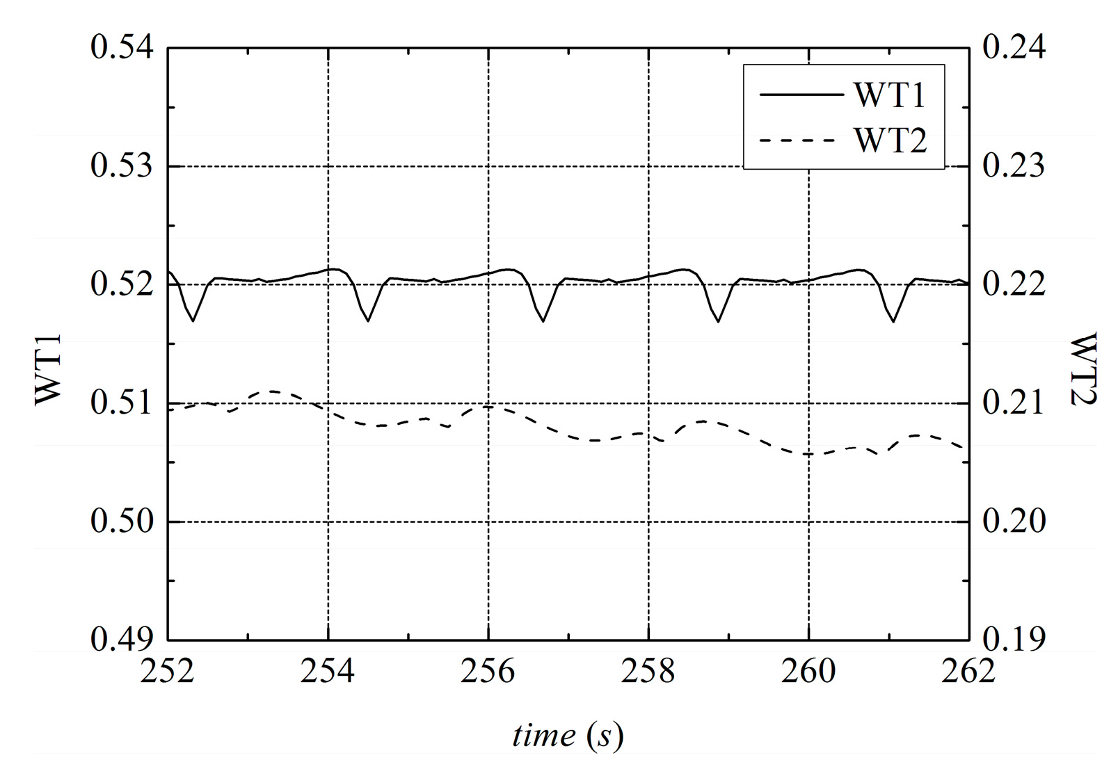
Figure 20.
Comparison of power coefficient between WT1 and WT2.
Figure 20.
Comparison of power coefficient between WT1 and WT2.
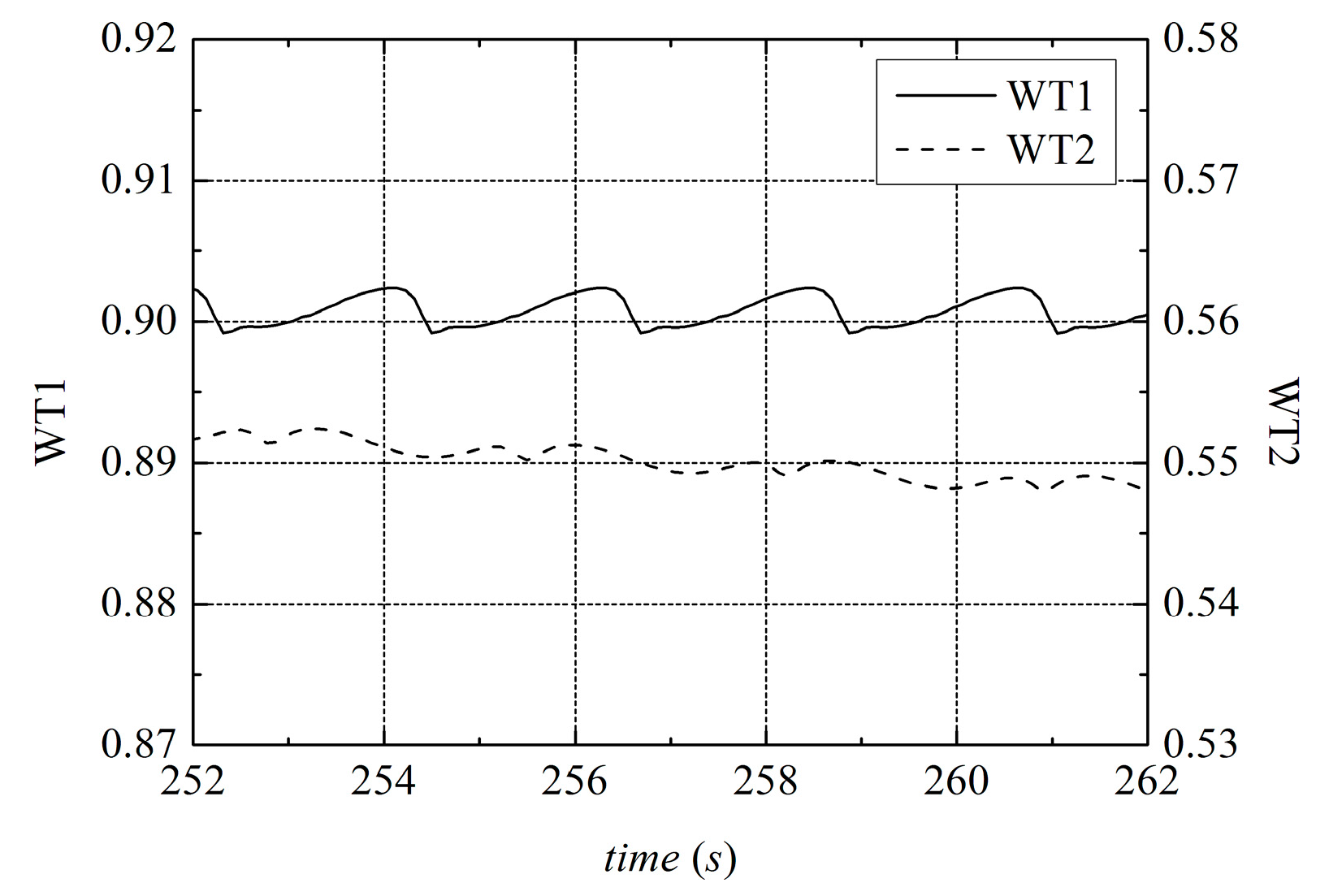
Figure 21.
Comparison of thrust coefficient between WT1 and WT2.
Figure 21.
Comparison of thrust coefficient between WT1 and WT2.
Figure 22.
Tangential and normal force distribution in radial direction: (a) WT1; (b) WT2.
Figure 22.
Tangential and normal force distribution in radial direction: (a) WT1; (b) WT2.
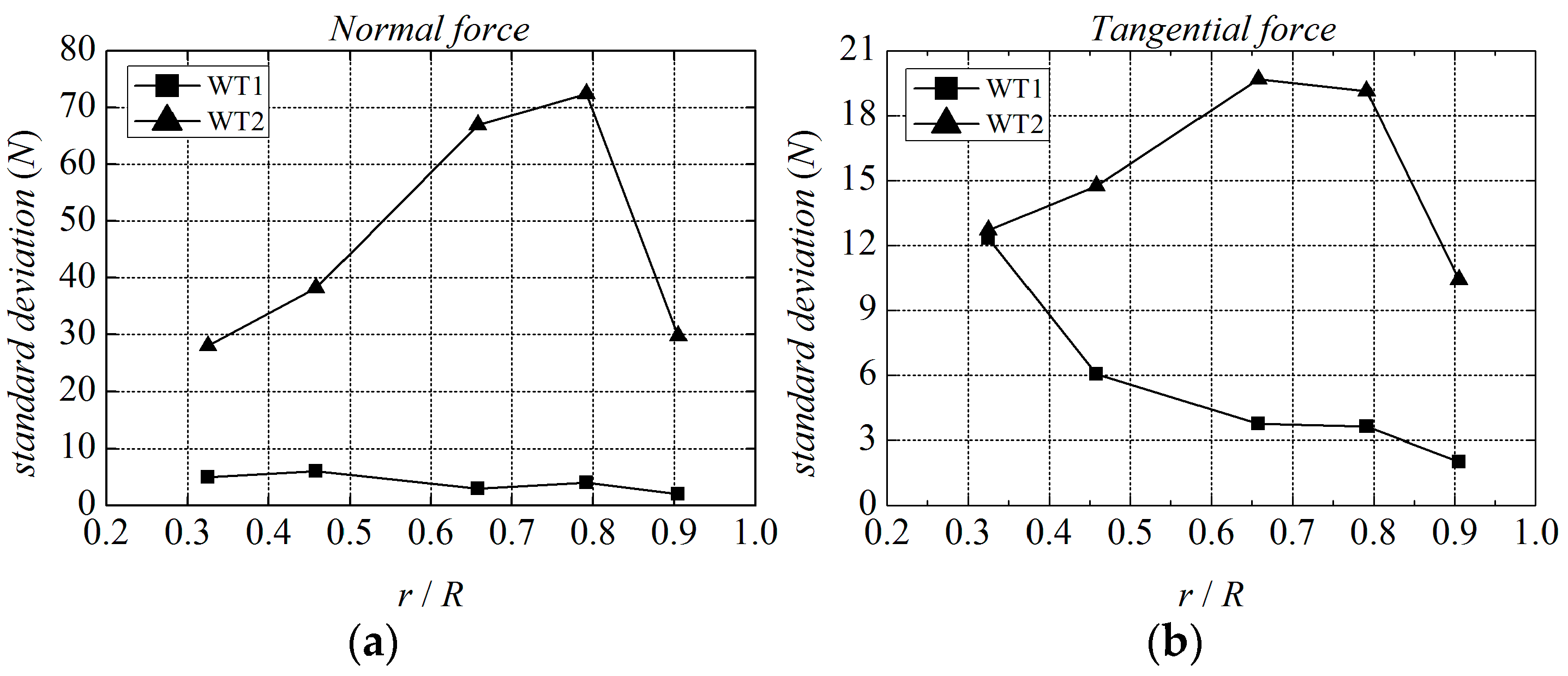
Figure 23.
Standard deviations of the normal and tangential force. (a) Normal force; (b) Tangential force.
Figure 23.
Standard deviations of the normal and tangential force. (a) Normal force; (b) Tangential force.
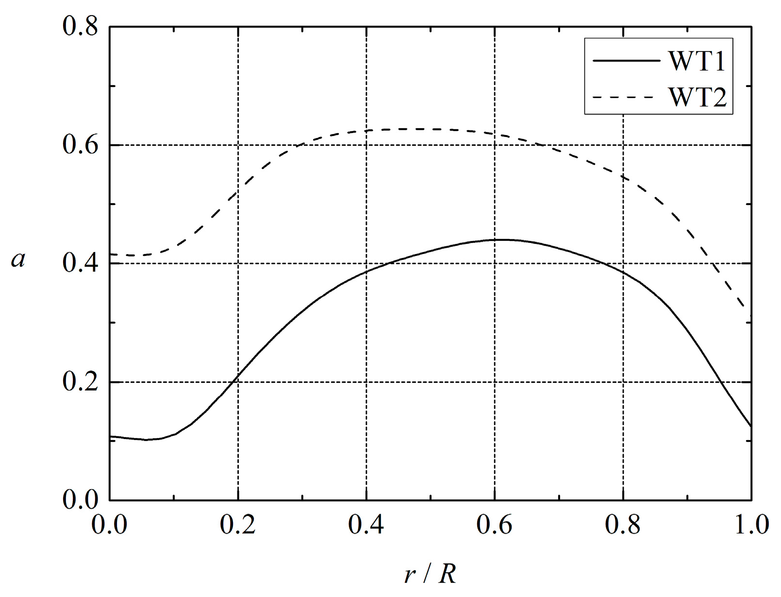
Figure 24.
Radial distributions of averaged axial flow interference factors.
Figure 24.
Radial distributions of averaged axial flow interference factors.
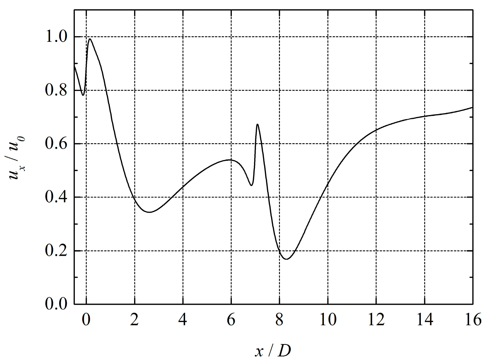
Figure 25.
Distributions of the average axial velocity at hub height.
Figure 25.
Distributions of the average axial velocity at hub height.
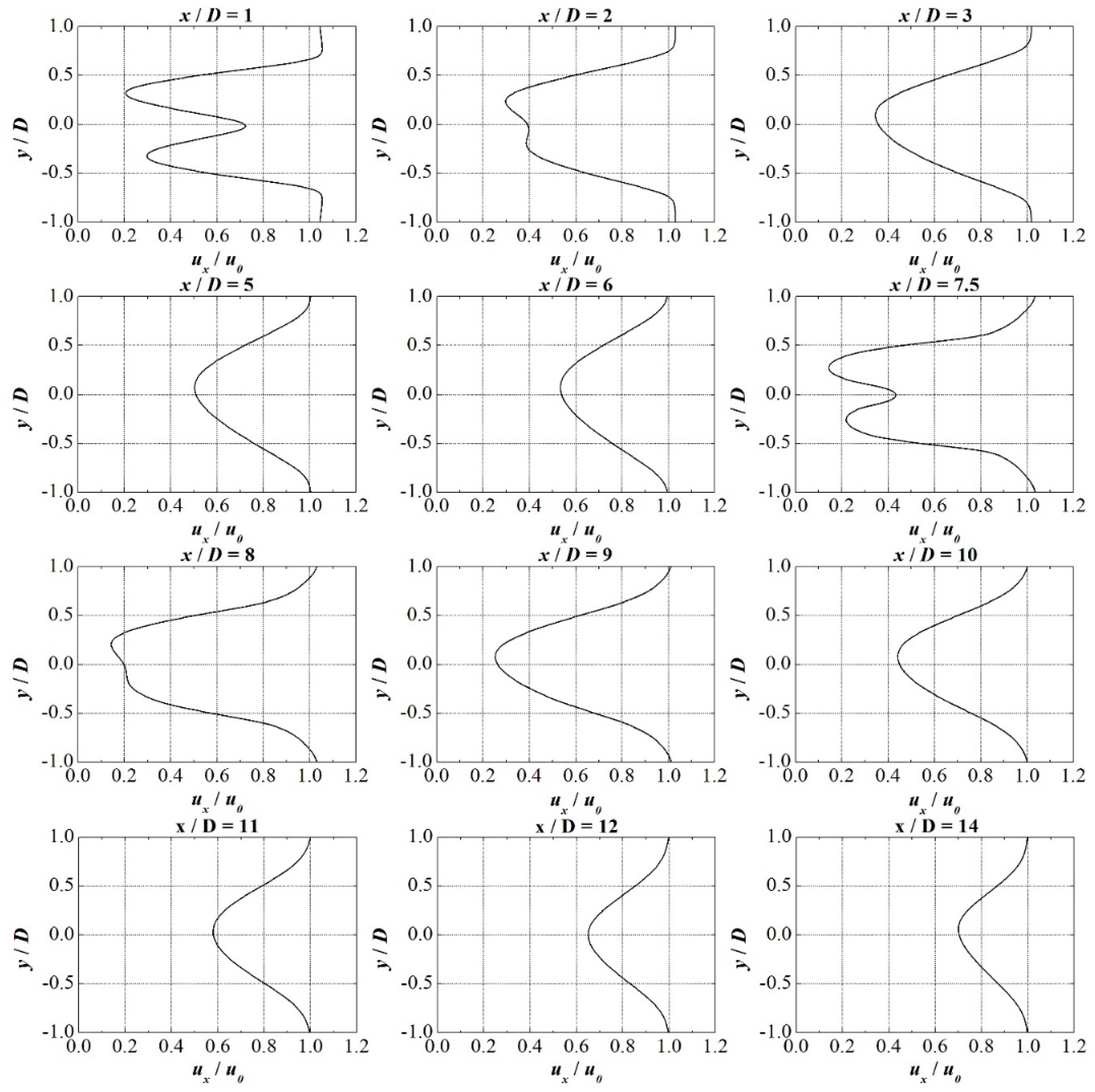
Figure 26.
Spanwise profile of average axial velocity at different locations.
Figure 26.
Spanwise profile of average axial velocity at different locations.
Table 1.
Distributed blade structural and aerodynamic properties.
Table 1.
Distributed blade structural and aerodynamic properties.
| Radius (m) | Chord (m) | Chord Mount | Airfoil Properties |
|---|
| 0.000 | 3.542 | 0.25 | - |
| 1.367 | 3.542 | 0.249 | Cylinder1 |
| 4.100 | 3.854 | 0.222 | Cylinder1 |
| 6.833 | 4.167 | 0.188 | Cylinder1 |
| 10.250 | 4.557 | 0.146 | Cylinder2 |
| 14.350 | 4.652 | 0.125 | DU 1 40 |
| 18.450 | 4.458 | 0.125 | DU35 |
| 22.550 | 4.249 | 0.125 | DU35 |
| 26.650 | 4.007 | 0.125 | DU30 |
| 30.750 | 3.748 | 0.125 | DU25 |
| 34.850 | 3.502 | 0.125 | DU25 |
| 38.950 | 3.256 | 0.125 | DU21 |
| 43.050 | 3.010 | 0.125 | DU21 |
| 47.150 | 2.764 | 0.125 | NACA 2 64 |
| 51.250 | 2.518 | 0.125 | NACA64 |
| 54.667 | 2.313 | 0.125 | NACA64 |
| 57.400 | 2.086 | 0.125 | NACA64 |
| 60.133 | 1.419 | 0.125 | NACA64 |
| 61.500 | 0.961 | 0.125 | NACA64 |
Table 2.
Mesh information of airfoil simulation.
Table 2.
Mesh information of airfoil simulation.
| ri | Ncells |
|---|
| 4° and 10° |
|---|
| 1.000 | 929,280 |
| 1.143 | 711,480 |
| 1.333 | 522,720 |
| 1.600 | 363,000 |
| 2.000 | 232,320 |
| 2.286 | 177,870 |
| 2.667 | 130,680 |
| 3.200 | 90,750 |
| 4.000 | 58,080 |
Table 3.
Lift () and drag () coefficients with different attack angles.
Table 3.
Lift () and drag () coefficients with different attack angles.
| ri | 4° | 10° |
|---|
| Cd | CL | Cd | CL |
|---|
| 4.000 | 9.599 × 10⁻³ | 4.342 × 10⁻¹ | 1.583 × 10⁻² | 1.058 |
| 3.200 | 9.484 × 10⁻³ | 4.346 × 10⁻¹ | 1.558 × 10⁻² | 1.060 |
| 2.667 | 9.325 × 10⁻³ | 4.353 × 10⁻¹ | 1.526 × 10⁻² | 1.062 |
| 2.286 | 9.326 × 10⁻³ | 4.352 × 10⁻¹ | 1.530 × 10⁻² | 1.061 |
| 2.000 | 9.348 × 10⁻³ | 4.351 × 10⁻¹ | 1.535 × 10⁻² | 1.061 |
| 1.600 | 9.263 × 10⁻³ | 4.353 × 10⁻¹ | 1.532 × 10⁻² | 1.062 |
| 1.333 | 9.224 × 10⁻³ | 4.357 × 10⁻¹ | 1.515 × 10⁻² | 1.063 |
| 1.143 | 9.226 × 10⁻³ | 4.356 × 10⁻¹ | 1.518 × 10⁻² | 1.063 |
| 1.000 | 9.230 × 10⁻³ | 4.356 × 10⁻¹ | 1.518 × 10⁻² | 1.063 |
Table 4.
The uncertainty of lift and drag coefficient with the grid refinement for different attack angles.
Table 4.
The uncertainty of lift and drag coefficient with the grid refinement for different attack angles.
| ri | 4° | 10° |
|---|
| UCd | UCL | UCd | UCL |
|---|
| 1.000 | 1.519 × 10⁻⁴ | 3.684 × 10⁻⁴ | 2.751 × 10⁻⁴ | 1.308 × 10⁻³ |
| 1.143 | 1.733 × 10⁻⁴ | 5.861 × 10⁻⁴ | 3.189 × 10⁻⁴ | 1.946 × 10⁻³ |
| 1.333 | 2.486 × 10⁻⁴ | 6.900 × 10⁻⁴ | 4.784 × 10⁻⁴ | 2.376 × 10⁻³ |
| 1.600 | 3.327 × 10⁻⁴ | 1.163 × 10⁻³ | 6.305 × 10⁻⁴ | 3.812 × 10⁻³ |
| 2.000 | 5.065 × 10⁻⁴ | 2.020 × 10⁻³ | 8.771 × 10⁻⁴ | 6.518 × 10⁻³ |
| 2.286 | 6.895 × 10⁻⁴ | 2.350 × 10⁻³ | 1.258 × 10⁻³ | 7.625 × 10⁻³ |
| 2.667 | 9.874 × 10⁻⁴ | 2.952 × 10⁻³ | 1.812 × 10⁻³ | 9.624 × 10⁻³ |
| 3.200 | 1.320 × 10⁻³ | 4.785 × 10⁻³ | 2.344 × 10⁻³ | 1.513 × 10⁻³ |
| 4.000 | 2.113 × 10⁻³ | 7.247 × 10⁻³ | 3.649 × 10⁻³ | 2.373 × 10⁻³ |
Table 5.
Range of exact lift and drag coefficient with the grid refinement for different attack angles.
Table 5.
Range of exact lift and drag coefficient with the grid refinement for different attack angles.
| ri | 4° | 10° |
|---|
| Cd | CL | Cd | CL |
|---|
| Cd − UCd | Cd + UCd | CL − UCL | CL + UCL | Cd − UCd | Cd + UCd | CL − UCL | CL + UCL |
|---|
| 1.000 | 9.078 × 10⁻³ | 9.382 × 10⁻³ | 4.352 × 10⁻¹ | 4.360 × 10⁻¹ | 1.491 × 10⁻² | 1.546 × 10⁻² | 1.061 | 1.064 |
| 1.143 | 9.052 × 10⁻³ | 9.399 × 10⁻³ | 4.350 × 10⁻¹ | 4.362 × 10⁻¹ | 1.486 × 10⁻² | 1.550 × 10⁻² | 1.061 | 1.065 |
| 1.333 | 8.976 × 10⁻³ | 9.473 × 10⁻³ | 4.350 × 10⁻¹ | 4.364 × 10⁻¹ | 1.467 × 10⁻² | 1.563 × 10⁻² | 1.060 | 1.065 |
| 1.600 | 8.931 × 10⁻³ | 9.596 × 10⁻³ | 4.341 × 10⁻¹ | 4.365 × 10⁻¹ | 1.469 × 10⁻² | 1.595 × 10⁻² | 1.058 | 1.066 |
| 2.000 | 8.841 × 10⁻³ | 9.855 × 10⁻³ | 4.331 × 10⁻¹ | 4.371 × 10⁻¹ | 1.447 × 10⁻² | 1.623 × 10⁻² | 1.055 | 1.068 |
| 2.286 | 8.637 × 10⁻³ | 1.001 × 10⁻² | 4.329 × 10⁻¹ | 4.376 × 10⁻¹ | 1.404 × 10⁻² | 1.656 × 10⁻² | 1.054 | 1.069 |
| 2.667 | 8.338 × 10⁻³ | 1.031 × 10⁻² | 4.323 × 10⁻¹ | 4.383 × 10⁻¹ | 1.345 × 10⁻² | 1.707 × 10⁻² | 1.052 | 1.071 |
| 3.200 | 8.163 × 10⁻³ | 1.080 × 10⁻² | 4.298 × 10⁻¹ | 4.394 × 10⁻¹ | 1.323 × 10⁻² | 1.792 × 10⁻² | 1.045 | 1.075 |
| 4.000 | 7.485 × 10⁻³ | 1.171 × 10⁻² | 4.269 × 10⁻¹ | 4.414 × 10⁻¹ | 1.219 × 10⁻² | 1.948 × 10⁻² | 1.034 | 1.081 |
Table 6.
The mesh independence test.
Table 6.
The mesh independence test.
| Number of Cell | Cp | Error (%) | Ct | Error (%) |
|---|
| 375,432 | 0.4678 | 5.864 | 0.8665 | 6.987 |
| 744,792 | 0.4642 | 5.047 | 0.8599 | 6.170 |
| 2,903,144 | 0.4634 | 4.858 | 0.8584 | 5.981 |
| 5,958,336 | 0.4627 | 4.715 | 0.8572 | 5.838 |
Table 7.
Comparison of the computed power and thrust between FAST and turbinesFoam at different wind speeds.
Table 7.
Comparison of the computed power and thrust between FAST and turbinesFoam at different wind speeds.
| Wind Speed (m/s) | Thrust of TurbinesFoam (kN) | Power of TurbinesFoam (MW) | Thrust of FAST (kN) | Power of FAST (MW) | Thrust Errors (%) | Power Errors (%) |
|---|
| 5.0 | 223.578 | 0.4400 | 264.9066 | 0.4236 | 15.60 | 3.88 |
| 6.0 | 288.945 | 0.8265 | 331.8101 | 0.7652 | 12.92 | 8.01 |
| 7.0 | 357.735 | 1.3088 | 397.2068 | 1.2240 | 9.94 | 6.92 |
| 8.0 | 433.465 | 1.9026 | 467.6329 | 1.8251 | 7.31 | 4.25 |
| 9.0 | 548.601 | 2.7090 | 577.9532 | 2.5955 | 5.08 | 4.37 |
| 10.0 | 677.285 | 3.7160 | 691.1475 | 3.5587 | 2.01 | 4.42 |
| 11.4 | 722.471 | 5.0363 | 803.9102 | 5.000 | 3.91 | 0.73 |
Table 8.
Comparison of the power with Glauert model and without the tip loss model.
Table 8.
Comparison of the power with Glauert model and without the tip loss model.
| Methods | Mean Power (MW) | Cp | Difference (%) |
|---|
| Glauert model | 5.243 | 0.4634 | 4.858 |
| No model | 5.600 | 0.4950 | 12.018 |
Table 9.
Comparison of the power and thrust.
Table 9.
Comparison of the power and thrust.
| Power (MW) | Difference (%) | Thrust (kN) | Error (%) |
|---|
| 1.9026 | 4.245 | 433.47 | 5.079 |
Table 10.
Power coefficient with different tip speed ratios of WT2.
Table 10.
Power coefficient with different tip speed ratios of WT2.
| Tip Speed Ratio of WT2 | Power Coefficient (WT1) | Power Coefficient (WT2) |
|---|
| 3.5 | 0.5206 | 0.0899 |
| 4.0 | 0.5205 | 0.1256 |
| 4.5 | 0.5205 | 0.1599 |
| 5.0 | 0.5204 | 0.1885 |
| 5.5 | 0.5204 | 0.2024 |
| 6.1 | 0.5203 | 0.2069 |
| 6.5 | 0.5203 | 0.2054 |
| 7.0 | 0.5202 | 0.1961 |
| 7.55 | 0.5201 | 0.1794 |
Table 11.
The mean power and ap with different turbine separations.
Table 11.
The mean power and ap with different turbine separations.
| Mean Power (MW) | Turbine 1 | Turbine 2 | ap (W/m) |
|---|
| 6D | 2.0312 | 0.6817 | 901.7270 |
| 7D | 2.0345 | 0.8089 | 917.1647 |
| 8D | 2.0336 | 0.9275 | 920.1591 |
Table 12.
The comparison of mean power computed by improved ALM. ALM: Actuator Line Model.
Table 12.
The comparison of mean power computed by improved ALM. ALM: Actuator Line Model.
| Mean Power (MW) | Turbine 1 | Turbine 2 |
|---|
| Jha | 1.9217 | 0.8644 |
| turbinesFoam | 2.0345 | 0.8089 |
| Error (%) | 5.87 | 6.42 |


