The Derivation of the Stability Bound of the Feedback ANC System That Has an Error in the Estimated Secondary Path Model

Abstract

This paper investigates the stability problem of the feedback active noise control (ANC) system, which can be caused by the modeling error of the electro-acoustic path estimation in its feedback mechanism. A stability analysis method is proposed to obtain the stability bound as a form of a closed-form equation in terms of the delay error length of the secondary path, the ANC filter length, and the primary noise frequency. In the proposed method, the system’s open loop magnitude and phase response equations are separately exploited and approximated within the Nyquist stability criterion. The stability bound of the proposed method is verified by comparing both the original Nyquist stability condition and the simulation results.

1. Introduction

Active noise control (ANC) is intended to suppress an external noise in an active way that an anti-noise with opposite phase and same magnitude cancels the external noise [1,2,3]. Feedforward ANC, which is the typical ANC scheme, captures a reference signal with a microphone at noise source to provide the input of the ANC system, which drives the anti-noise. Unlike the feedforward ANC, feedback active noise control (FBANC) does not need a microphone or sensor to install at noise source for a reference signal but utilizes a feedback mechanism to internally generate a reference signal. The structure of the feedback ANC is considered as one of the typical internal model control (IMC) in the sense that the estimated model of the secondary path is used for the generation of a reference signal [2]. For this structural nature, in applications where noise sources are many and propagation paths of noises are unspecified, e.g., ANC headphones, the feedback ANC is preferred to be implemented rather than the feedforward scheme, in which independent reference sensors need to be installed [4,5,6].

In practical feedback ANC applications, the stability problem caused by the feedback mechanism is an important issue in the design and implementation. In the feedback mechanism, there are an electro-acoustic coupling path and its estimated model, which is in a form of an FIR filter. The electro-acoustic coupling path called the secondary path includes a loud speaker, a microphone, an acoustic propagation path, and AD/DA converters.

The feedback ANC structure is reduced to the feedforward structure provided the secondary path model is perfect. Theoretically, if the secondary path model is perfectly estimated, the feedback ANC scheme has no stability problem [2,3,4]. However, in practice, it is not available to exactly estimate them as a linear filter model, since the electro-acoustic devices and the acoustic path are a non-linear and time-varying system [3,7,8,9]. If the estimated secondary path model is not perfect, its adverse effects considering both the stability aspect of the feedback loop and the performance issues, such as convergence and stability, of the FXLMS-based adaptive algorithm must be analyzed. The previous research [7] gives examples of combined analysis to show the convergence stability of adaptive active noise control systems. There are, in the literature, some analyses showing how to guarantee convergence of the feedfowards FXLMS without secondary path modeling by applying varying-delay LMS approach, or fuzzy approach [10,11]. However, it is true that the comprehensive analysis of the FXLMS-based feedback ANC considering all the feedback structural aspects is generally a hard problem. The difficulty is caused by its inherent structural complexity and, as well, by the difficulty of reflecting the wide range of environmental variations of ANC application.

This paper exclusively discusses the stability aspect of the feedback loop to derive a closed-form stability bound equation of the feedback ANC system with a delay mismatch in the secondary path model. The availability of the stability bound in a form of closed equation, relating with various physical domain design factors such as noise characteristics, or system parameters, would be very helpful for practical feedback ANC applications.

A typical method to determine the stability of feedback systems is to examine the pole locations of a system’s characteristic equation. In many applications of feedback ANC system, it is not possible to directly obtain the roots of the characteristic equation, because the equation is generally of a very high order [2]. Particularly, the delay of the acoustic path, which is relatively long compare to that of the electric path, makes the order of the characteristic equation even higher. Therefore, many literatures on the stability analysis of feedback ANC systems have been analyzed using the frequency domain analysis approach [3,7,8]. However, the stability bound result is shown in the transfer function model domain, which reflects, indirectly, the effect of the physical domain parameters such as delay length of an acoustic system, ANC filter length, and center frequency of target noise. In [3], the effects of each error in the parameters of secondary path model are treated as a single transfer function model. The upper bound of secondary path model error is also obtained as a transfer function bound that defines the magnitude bounds for each frequency. In [7], though the effects of the errors in magnitude response and pure delay components are treated separately in the analysis, the effect of the delay error of the estimated secondary path model is not treated in the analysis.

Another appropriate frequency response approach for stability analysis of the feedback system is the Nyquist stability determining technique [12,13]. In the Nyquist criterion, a feedback system’s stability is guaranteed when the polar plot of the open loop frequency response does not enclose the Nyquist point (−1, 0) for any frequency. The Nyquist technique is basically considered as a trial-and-error based approach, in which the stability bound can be obtained through direct drawing of polar plots by changing the values of the parameters.

In this paper, we derive a stability bound equation in terms of the delay error of the secondary path model, the ANC filter length, and the target noise’s frequency. This paper is considered as a major extension of the authors’ previous work [8], which can be considered as an incomplete work to reflect only the magnitude response of the system’s open loop response in deriving the system’s stability bound. This paper provides a more realistic stability bound by exploiting both the magnitude and phase of the FBANC system’s open loop response in deriving the stability bound equation. The magnitude and phase response equations of the open loop function of the feedback ANC, which guarantee the Nyquist stability criterion, are approximated as linear equations and combined. In the derivation process, we use several assumptions in which the primary noise is a single-tone sinusoid and the secondary path is modeled as pure delay. The exclusion of the magnitude mismatch effect of secondary path model is considered acceptable in narrowband ANC applications, while it would not be acceptable in cases of wideband ANC applications.

One of the significant advantages compared to the Nyquist technique is that the closed-form equation can provide the fast computation of parameter bounds. The real-time computation of the stability bounds is expected to be useful for the design and operation of the feedback ANC system. The obtained stability bounds are verified by comparison with both the original Nyquist stability condition and the simulation results. Simulations with a practical secondary path measured from commercial headphones are also added to verify the analysis based on the assumption of the pure delay model.

2. The Stability Problem of the Feedback ANC System

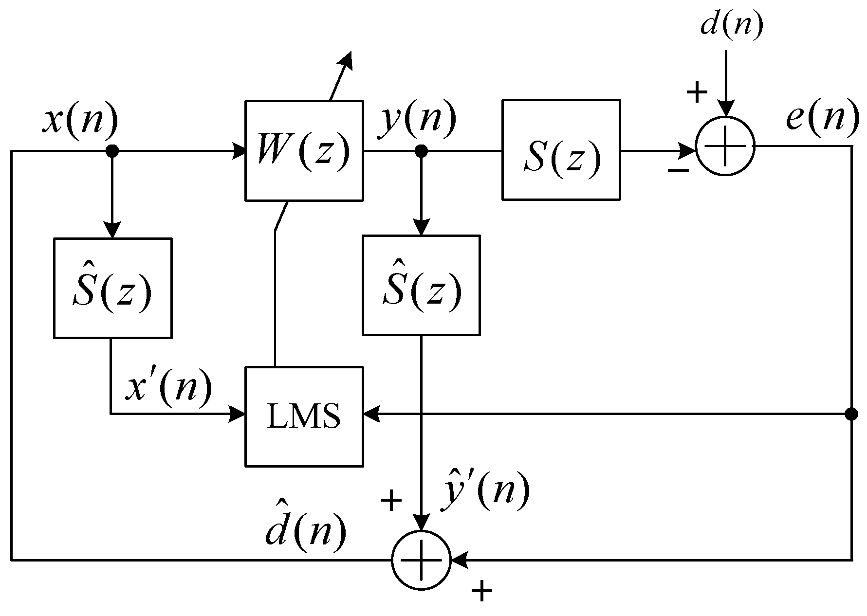
In this section, we address the stability issue caused by the secondary path modeling error of a feedback ANC system. A typical structure of an adaptive feedback ANC using the FXLMS system [1] is shown in Figure 1. The basic idea of the adaptive feedback ANC is to estimate the primary noise d(n) and use it as a reference signal x(n) for the ANC filter. The reference signal x(n) is synthesized using the estimate of secondary path model $\widehat{S}(z)$ as shown in (1). The feedback ANC system suppresses primary noise d(n) by generating anti-noise y(n) with a loud speaker. Signal e(n) denotes residual noise measured by an error microphone.

$$\widehat{d}(n)={\widehat{y}}^{\prime }(n)+e(n)=y(n)\ast \widehat{s}(n)+e(n)\equiv x(n).$$

(1)

The followings are the rest of definitions.

• W(z): N-tap adaptive filter,
• S(z): Secondary path, the electro-acoustic coupling path from the loudspeaker to the error microphone,
• $\widehat{S}(z)$: The internal estimated model of S(z).

Stability of a linear feedback system can be determined by examining whether its overall transfer function’s pole locations are within the unit circle. The FBANC system’s closed-loop transfer function from desired input d(n) to error output e(n) can be obtained as,

$$H(z)=\frac{E(z)}{D(z)}=\frac{1-W(z)\widehat{S}(z)}{1+W(z)[S(z)-\widehat{S}(z)]}.$$

(2)

When there is no error in the estimated secondary path model, $\widehat{S}(z)=S(z)$, the denominator of (2), becomes one and the overall transfer function H(z) becomes

$$H(z)=1-W(z)\widehat{S}(z)=1-W(z)S(z).$$

in which the FBANC system has no poles and becomes an all-zero system that guarantees its stability. However, when the estimated secondary path $\widehat{S}(z)$ has an error, the denominator of (2) becomes a high order equation. This is because the adaptive filter W(z) is generally tens to hundreds order, and the secondary path S(z) and its estimation $\widehat{S}(z)$ also contain a very long delay because of the acoustical propagation path.

In order to examine the effect of the delay error explicitly, the transfer functions of the secondary path and its estimated model are modeled as a simple delay component as $S(z)=z^{-\Delta }$ and $\widehat{S}(z)=z^{-\widehat{\Delta }}$, respectively. The constant magnitude component of the both secondary path models can be accommodated in the adaptive filter model W(z). The delay $\Delta$ corresponds to the total time, including the acoustic propagation time between the speaker and microphone, as well as the AD/DA converting processing, which generally ranges hundreds of microseconds to tens of milliseconds. By substituting the delay models for H(z), the transfer function can be expressed as

$$H(z)=\frac{1-W(z)z^{-\widehat{\Delta }}}{1+W(z)[z^{-\Delta }-z^{-\widehat{\Delta }}]}.$$

(3)

This result transfer function shows the full behavior of the system that has a delay error in its secondary path model. However, from this function, it is hard to recognize the effect of delay error intuitively, since the transfer function-based expression does not directly provide explicit and geometric interpretations in the domain of physical parameters, such as delay, noise characteristics parameters [4]. Moreover, the combined effect of the adaptive filter W(z) on the secondary path error term is determined depending on characteristics of the primary noise d(n). In the next section, we introduce a new stability analysis method to obtain a stability bound equation that intuitively represents the effect of the physical parameters on the system stability.

3. Stability Analysis of Feedback ANC System

A new stability analysis method is proposed to obtain the stability bound of the feedback ANC system as a form of a closed-form equation. The closed-form stability bound equation is derived in terms of the length of the delay error of secondary path, the ANC filter length, and the frequency of a single-tone primary noise. In the proposed method, the stability bound equation is obtained by separating the magnitude and phase response equations of the open loop function $W(e^{j\omega })[e^{-j\omega \Delta }-e^{-j\omega \widehat{\Delta }}]$ within the Nyquist stability bound and exploiting their linear approximation. The magnitude and phase response equations are approximated as linear equations, assuming that the primary noise is a single-tone sinusoid and the secondary path can be modeled as a pure delay.

The stability definition of the Nyquist criterion is that the polar plot of the open loop frequency response must not enclose the Nyquist point (−1, 0) for all frequency range [12,13]. Instead of this original Nyquist definition, we introduce an alternative stability definition that the magnitude of the open loop frequency response must be less than one at the specific frequency point ${\omega }_{180}$, which makes the phase of the open loop frequency response equal $\pm \pi$. From the proposed stability definition, the FBANC system’s stability can be guaranteed when the following formula is satisfied.

$$|W(e^{j\omega })|\cdot |e^{-j\omega \Delta }-e^{-j\omega \widehat{\Delta }}|{}_{\omega ={\omega }_{180}}<1.0,$$

(4)

in which the frequency point ${\omega }_{180}$ can be expressed as

$${\angle W(e^{j\omega })[e^{-j\omega \Delta }-e^{-j\omega \widehat{\Delta }}]|}_{\omega ={\omega }_{180}}=\pm \pi .$$

At the frequency point ${\omega }_{180}$, the open-loop frequency response $W(e^{j\omega })[e^{-j\omega \Delta }-e^{-j\omega \widehat{\Delta }}]$ is on the real-axis of z-plane.

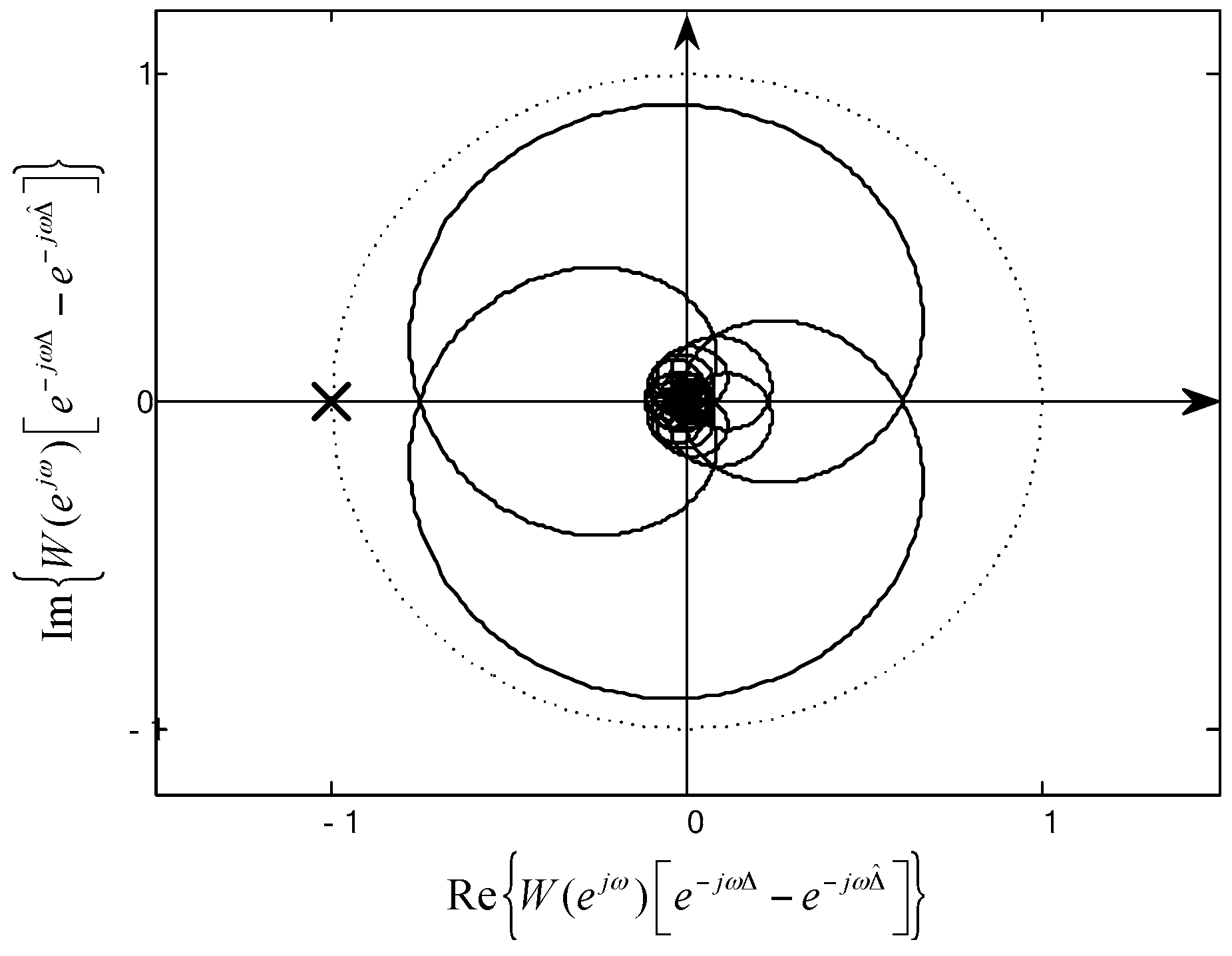
In Figure 2, an example Nyquist plot of the feedback ANC system (solid line) is drawn within unit circle (dotted line) on z-plane. The proposed stability definition is well-described with this example figure. If the Nyquist plot’s most left cross point on the real-axis does not reach the Nyquist point (−1, 0), the open loop frequency response never encloses the Nyquist point so that the Nyquist stability criterion always is guaranteed.

With the assumption that the adaptive algorithm converges to a stationary point and the primary noise is one of the specific types, i.e., pure-tone sinusoid or auto-regressive process model, each of the two magnitude responses, i.e., $|W(e^{j\omega })|$ and $|e^{-j\omega \Delta }-e^{-j\omega \widehat{\Delta }}|$, can be represented as a combined pattern using typical functions, i.e., a single sinusoid, a sinc function, or a quadratic function.

To derive the close-form equation of the stability bound, each term of the magnitude responses is linearized at the point where the magnitude response of $|e^{-j\omega \Delta }-e^{-j\omega \widehat{\Delta }}|$ alone becomes 1.0. Such approximation guarantees conservative bound of stability. However, the approximated stability bound is not significantly different from the true bound as verified through simulations in Section 5, which results from the fact that the term $|e^{-j\omega \Delta }-e^{-j\omega \widehat{\Delta }}|$ always dominates with faster varying characteristics of magnitude response than $|W(e^{j\omega })|$. Then, the overall magnitude response, i.e., the product of the two linearized terms, becomes a quadratic function. By finding the range for the quadratic equation to be less than 1.0, the stability bound is readily derived.

A significant feature of the proposed stability determination method is that it enables the analytic derivation of the stability bound equation without obtaining the roots of the characteristic equation, which is generally high-order. The proposed stability analysis method can be also utilized for other feedback control applications’ stability bound derivation.

4. Derivation of the Stability Bound of the Feedback ANC System

In this section, the closed-form stability bound equation is derived by utilizing the magnitude response and phase response of the two terms of the open-loop frequency response, i.e., $W(e^{j\omega })$ and $[e^{-j\omega \Delta }-e^{-j\omega \widehat{\Delta }}]$.

The frequency response of the adaptive filter $W(e^{j\omega })$ can be specified as a simple formation in assumption that the primary noise d(n) is a single-tone sinusoid $d(n)=\cos (\omega n+\varphi )$, and the coefficients of the ANC filter $W(e^{j\omega })$ converge to the optimum state [8]. Where, $\omega$ is frequency of the single-tone primary noise d(n) and $\varphi$ is phase. The optimum filter response for the single tone noise d(n) can be obtained from (3) as

$$W_o(e^{j\omega })=e^{j\omega \widehat{\Delta }},$$

(5)

which represents a pure time-advance system obtained by making the overall frequency response become zero at the frequency of the primary noise as $H(e^{j\omega })=0$.

For the single-tone signal that has a fixed frequency ${\omega }_0$, i.e., $d(n)=\cos ({\omega }_{0}n+\varphi )$, the frequency response at ±${\omega }_0$ is $W_o(e^{\pm j{\omega }_0})=e^{\pm j{\omega }_0\widehat{\Delta }}$. Then, the frequency response to the single-tone d(n), $W_o(e^{j\omega })$, can be considered as a summation of the two complex-valued phase delay terms at ±${\omega }_0$ as

$$W_o(e^{j\omega })=\frac{1}{2}\left[\delta (\omega -{\omega }_0)e^{j{\omega }_0\widehat{\Delta }}+\delta (\omega +{\omega }_0)e^{-j{\omega }_0\widehat{\Delta }}\right]$$

(6)

Therefore, the time-domain filter coefficients $w_0\left(n\right)$ are obtained as inverse Fourier transform of (6) as,

$$\begin{array}{ll}{w}_o(n)& =\frac{1}{2}\left[e^{j{\omega }_{0}n}\cdot e^{j{\omega }_0\widehat{\Delta }}+e^{-j{\omega }_{0}n}\cdot e^{-j{\omega }_0\widehat{\Delta }}\right]=\frac{1}{2}\left[e^{j{\omega }_0(n+\widehat{\Delta })}+e^{-j{\omega }_0(n+\widehat{\Delta })}\right]\\ & =\cos ({\omega }_{0}n+\widehat{\Delta }).\end{array}$$

The coefficients of the N-tap FIR ANC filter for the optimum response is obtained by applying N-tap rectangular window $w_R(n)$ as

$$w_o(n)=\{\begin{array}{ll}\frac{2}{N}\cos [{\omega }_0(n+\widehat{\Delta })]\hfill & forn=0,1,\cdots ,N-1\hfill \\ 0\hfill & \mathrm{elsewhere}\hfill \end{array},\hspace{1em}=\cos [{\omega }_0(n+\widehat{\Delta })]\cdot w_R(n).$$

(7)

in which,

$$w_R(n)=\{\begin{array}{ll}\frac{2}{N}\hfill & forn=0,1,\cdots ,N-1\hfill \\ 0\hfill & \mathrm{elsewhere}.\hfill \end{array}$$

The overall frequency response of the optimum ANC filter $W_o(e^{j\omega })$ can be expressed as the convolution of the discrete-time Fourier transform of the cosine function and that of the rectangular window as

$$W_o\left(e^{j\omega }\right)=\mathcal{F}\left[\cos [{\omega }_0(n+\widehat{\Delta })]\right]*\mathcal{F}\left[w_{R.i}\right].$$

in which $\mathcal{F}[\cdot ]$ is the discrete-time Fourier transform operation and $\ast$ is the convolution operator.

The discrete-time Fourier transform of the cosine term is obtained as

$$\mathcal{F}\left[\cos [{\omega }_0(n+\widehat{\Delta })]\right]=\frac{e^{j{\omega }_0\widehat{\Delta }}}{2}\delta (\omega -{\omega }_0)+\frac{e^{-j{\omega }_0\widehat{\Delta }}}{2}\delta (\omega +{\omega }_0)$$

The discrete-time Fourier transform of the rectangular window function is obtained as

$$\mathcal{F}\left[w_{R.i}\right]=e^{-j\frac{N-1}{2}\omega }\frac{\frac{2}{N}\sin \left(\frac{N}{2}\omega \right)}{\sin \left(\frac{1}{2}\omega \right)}$$

The overall frequency response of the optimum ANC filter $W_o(e^{j\omega })$ can be expressed as

$$\begin{array}{l}{W}_o(e^{j\omega })=\mathcal{F}\left[\cos [{\omega }_0(n+\widehat{\Delta })]\right]*\mathcal{F}\left[w_{R.i}\right]\\ =e^{-j\left[\frac{N-1}{2}(\omega -{\omega }_0)-{\omega }_0\widehat{\Delta }\right]}\frac{\sin \left[\frac{N}{2}\left(\omega -{\omega }_0\right)\right]}{N\sin \left[\frac{1}{2}\left(\omega -{\omega }_0\right)\right]}+e^{-j\left[\frac{N-1}{2}(\omega +{\omega }_0)+{\omega }_0\widehat{\Delta }\right]}\frac{\sin \left[\frac{N}{2}\left(\omega +{\omega }_0\right)\right]}{N\sin \left[\frac{1}{2}\left(\omega +{\omega }_0\right)\right]}\end{array}$$

(8)

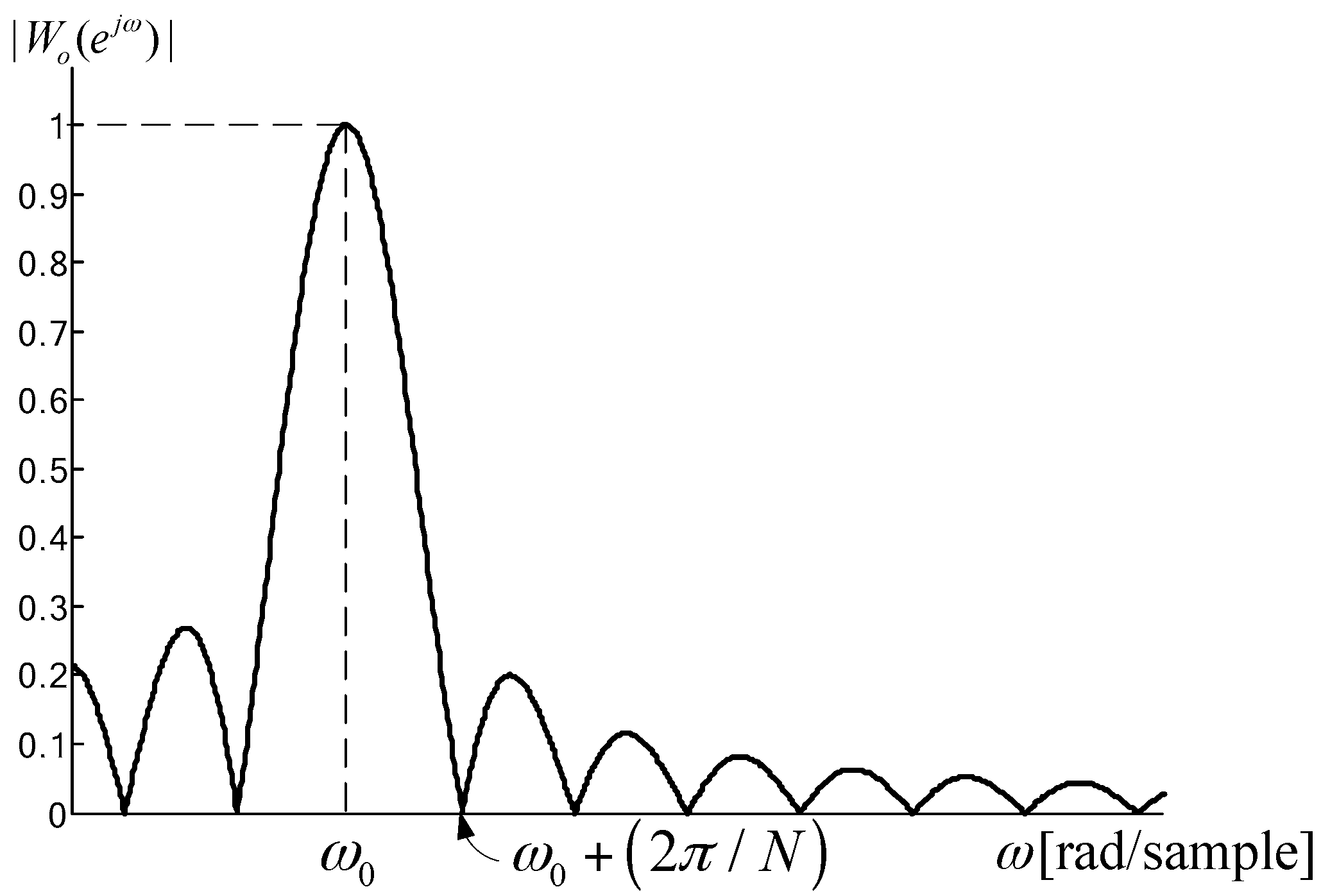
In (8), the frequency response of the ANC filter $W_o(e^{j\omega })$ can be viewed as two sinc functions shifted onto $\omega ={\omega }_0$ and $\omega =-{\omega }_0$, respectively.

When we assume that the filter length N is long enough to accommodate a single period of the primary noise, i.e., $N·2\pi /{\omega }_0$, the effect of the second term of the optimum ANC filter is negligibly small in the frequency range of the first term’s main lobe, i.e., ${\omega }_0-\frac{2\pi }{N}<\omega <{\omega }_0+\frac{2\pi }{N}$. An example of the magnitude response of the optimum ANC filter $|W_o(e^{j\omega })|$ is illustrated in Figure 3.

For the frequency range of the first term’s main lobe, the magnitude response of the optimum ANC filter can be approximated as

$$|W_o(e^{j\omega })|\cong \left|\sin \mathrm{c}\left[\frac{N}{2}\left(\omega -{\omega }_0\right)\right]+\delta \right|,$$

(9)

in which $\delta$ is a constant value to approximate the effect of second term of (8) on the magnitude response. The constant value is chosen as its potential maximum value existing in the right half of the main lobe as expressed as

$$\delta =\frac{1}{N\sin \left[{\omega }_0\right]}.$$

(10)

Since we assume that the filter length N is long enough to cover a single period of the primary noise $N·2\pi /{\omega }_0$, the potential effect of the second term of (8) is negligibly small for the frequency range of the first term’s main lobe. Therefore, the phase response $\angle W(e^{j\omega })$ within the frequency range of the first term’s main lobe, i.e., ${\omega }_0-\frac{2\pi }{N}<\omega <{\omega }_0+\frac{2\pi }{N}$, can be approximated as

$$\angle W_o(e^{j\omega })\cong -\frac{N-1}{2}\omega +\left(\widehat{\Delta }+\frac{N-1}{2}\right){\omega }_0,\mathrm{for}{\omega }_0-\frac{2\pi }{N}<\omega <{\omega }_0+\frac{2\pi }{N}.$$

(11)

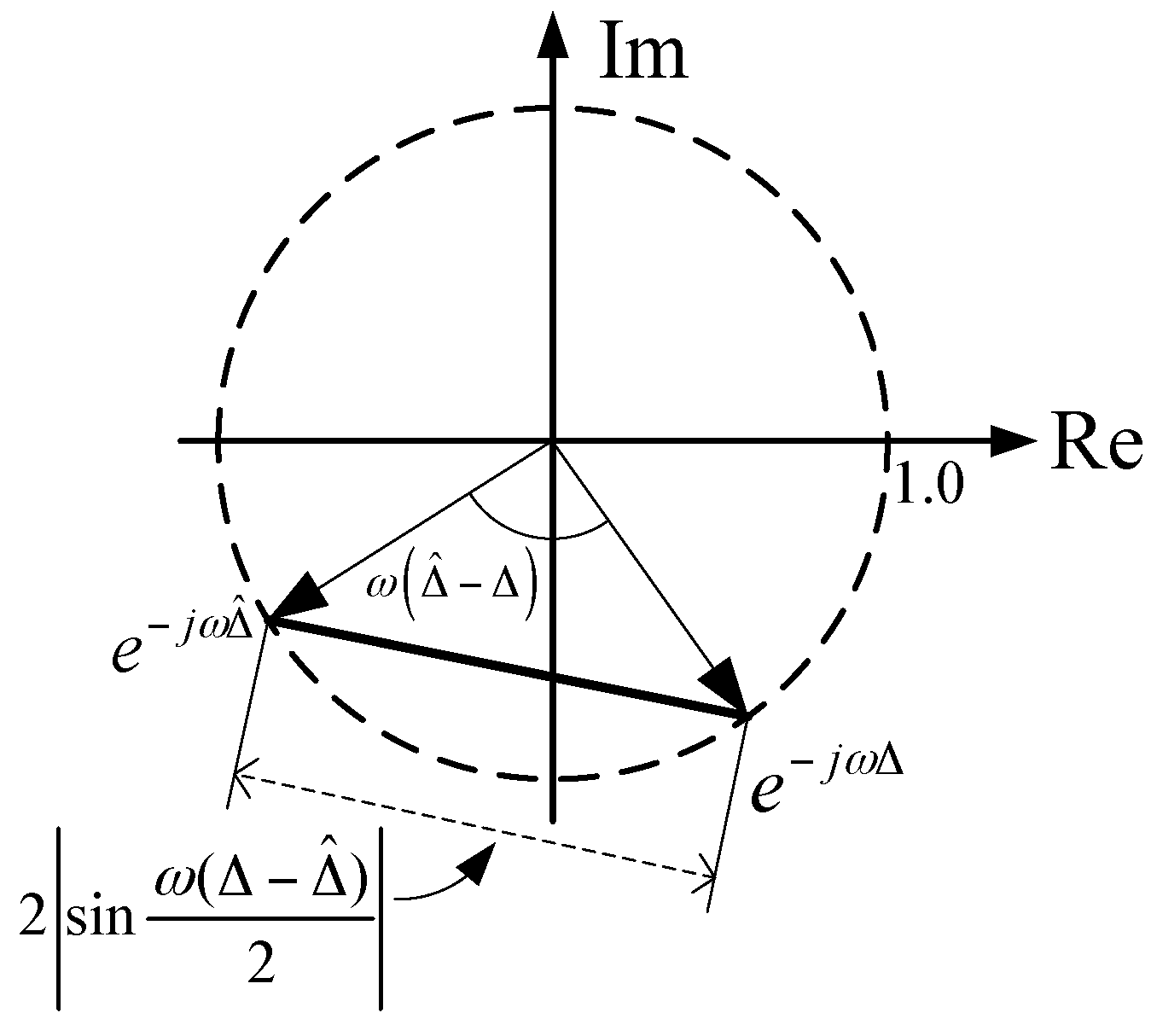
The second term of the open loop frequency response $[e^{-j\omega \Delta }-e^{-j\omega \widehat{\Delta }}]$ can be derived as

$$e^{-j\omega \Delta }-e^{-j\omega \widehat{\Delta }}=2j\sin \frac{\omega (\Delta -\widehat{\Delta })}{2}\cdot e^{-j\frac{\omega (\Delta +\widehat{\Delta })}{2}}.$$

(12)

The second term’s magnitude response $|e^{-j\omega \Delta }-e^{-j\omega \widehat{\Delta }}|$ can be viewed as a length of base of an isosceles triangle that has unit-length legs and a vertex angle $\mathsf{\omega },$ as shown in Figure 4, and can be expressed as

$$|e^{-j\omega \Delta }-e^{-j\omega \widehat{\Delta }}|=2\cdot \left|\sin \frac{\omega (\Delta -\widehat{\Delta })}{2}\right|.$$

(13)

The phase response $\angle [e^{-j\omega \Delta }-e^{-j\omega \widehat{\Delta }}]$ is obtained as

$$\angle [e^{-j\omega \Delta }-e^{-j\omega \widehat{\Delta }}]=\{\begin{array}{c}-\frac{\omega (\Delta +\widehat{\Delta })}{2}-\frac{\pi }{2}\mathrm{for}\Delta >\widehat{\Delta },\\ -\frac{\omega (\Delta +\widehat{\Delta })}{2}+\frac{\pi }{2}\mathrm{for}\Delta <\widehat{\Delta }.\end{array}$$

(14)

For the case of $\Delta >\widehat{\Delta }$, the overall phase response can be obtained by summing the separate phase responses (11) and (14) as

$$\begin{array}{l}\angle W(e^{j\omega })[e^{-j\omega \Delta }-e^{-j\omega \widehat{\Delta }}]=\angle W(e^{j\omega })+\angle [e^{-j\omega \Delta }-e^{-j\omega \widehat{\Delta }}]\\ =-\frac{\Delta +\widehat{\Delta }+N-1}{2}\omega +\frac{2\widehat{\Delta }+N-1}{2}{\omega }_0-\frac{\pi }{2}.\end{array}$$

(15)

From (15), the frequency point ${\omega }_{180}$, where the phase response $\angle W(e^{j\omega })[e^{-j\omega \Delta }-e^{-j\omega \widehat{\Delta }}]$ equals $\pm \pi$, is obtained as

$${\omega }_{180}={\omega }_0+\frac{\pi -(\Delta -\widehat{\Delta }){\omega }_0}{\Delta +\widehat{\Delta }+N-1}={\omega }_0+\lambda .$$

(16)

The overall magnitude response can be obtained using (9) and (13) as following.

$$\begin{array}{l}|W(e^{j\omega })|\cdot |e^{-j\omega \Delta }-e^{-j\omega \widehat{\Delta }}|\\ \cong \left|\sin \mathrm{c}\left(\frac{N}{2}\left[\omega -{\omega }_0\right]\right)+\delta \right|\cdot 2\left|\sin \frac{\omega (\Delta -\widehat{\Delta })}{2}\right|\end{array}.$$

(17)

By using (16) and (17), the proposed stability formula (4) is derived as

$$\begin{array}{l}|W(e^{j\omega })|\cdot |e^{-j\omega \Delta }-e^{-j\omega \widehat{\Delta }}|{}_{\omega ={\omega }_{180}}\\ \cong \left|\sin \mathrm{c}\left(\frac{N\lambda }{2}\right)+\delta \right|\cdot 2\left|\sin \frac{{\omega }_{180}(\Delta -\widehat{\Delta })}{2}\right|=\left|\sin \mathrm{c}\left(\frac{N\lambda }{2}\right)+\delta \right|\cdot 2\left|\sin \frac{\lambda +{\omega }_0}{2}\frac{\pi -\lambda (2\widehat{\Delta }+N-1)}{\lambda +{\omega }_0}\right|\\ =\left|\sin \mathrm{c}\left(\frac{N\lambda }{2}\right)+\delta \right|\cdot 2\left|\sin \left(\frac{\pi }{2}-\frac{\lambda (2\widehat{\Delta }+N-1)}{2}\right)\right|=2\left|\sin \mathrm{c}\left(\frac{N\lambda }{2}\right)+\delta \right|\cdot \left|\cos \left(\frac{\lambda (2\widehat{\Delta }+N-1)}{2}\right)\right|.\end{array}$$

(18)

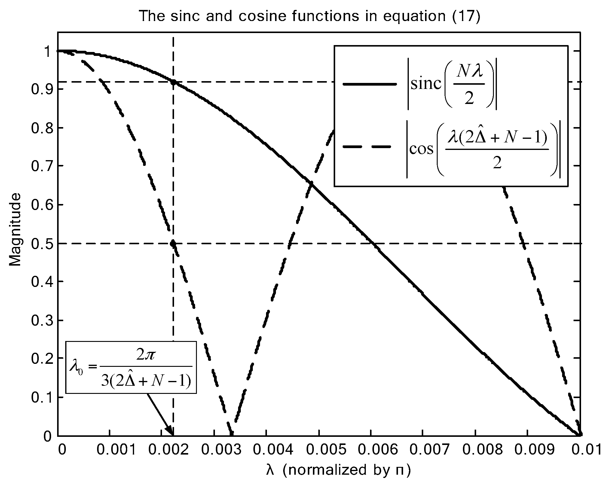
In Figure 5, examples of the sinc function and the cosine function terms of (18) are illustrated on $\lambda$-axis. Each first zero crossing points of the sinc function and the cosine function are located at $\lambda =2\pi /N$ and $\lambda =\pi /\left(2\Delta ^+N-1\right)$, respectively. From (18), the stability bound is expected to be around $\lambda =2\pi /3\left(2\Delta ^+N-1\right)$, in which the cosine function becomes 0.5 and the sinc function is slightly smaller than 1.0. We simplify the sinc function and the cosine function into 1st order linear equations by performing the Taylor expansion at the point ${\lambda }_0=2\pi /3\left(2\Delta ^+N-1\right)$ as

$$\begin{array}{l}\sin c\left(\frac{N\lambda }{2}\right)+\delta \cong \\ \sin c\left(\frac{N{\lambda }_0}{2}\right)+\frac{N}{2}\left\{\frac{\cos (\frac{N{\lambda }_0}{2})}{\frac{N{\lambda }_0}{2}}-\frac{\sin (\frac{N{\lambda }_0}{2})}{{\left(\frac{N{\lambda }_0}{2}\right)}^2}\right\}\left(\lambda -{\lambda }_0\right)+\delta \end{array}$$

(19)

$$\cos \left(\frac{\lambda (2\widehat{\Delta }+N-1)}{2}\right)\cong \frac{1}{2}-\frac{1}{{\lambda }_0}\frac{\pi }{2\sqrt{3}}\left(\lambda -{\lambda }_0\right)$$

(20)

The proposed stability bound can be simplified into a quadratic equation by substituting (19) and (20) into (18) as

$$\frac{2}{N{\lambda }_0}\left[\sin \frac{N{\lambda }_0}{2}+\frac{N{\lambda }_0\delta }{2}-\frac{N\rho }{2}(\lambda -{\lambda }_0)\right]\cdot \left[1-\frac{\pi }{\sqrt{3}{\lambda }_0}(\lambda -{\lambda }_0)\right]<1.0,$$

(21)

in which

$$\rho =\frac{2}{N{\lambda }_0}\sin \frac{N{\lambda }_0}{2}-\cos \frac{N{\lambda }_0}{2}.$$

This quadratic equation is satisfied when

$$\lambda >{\lambda }_0\left[1+\frac{\gamma }{{\lambda }_0}+\frac{\sqrt{3}}{2\pi }-\sqrt{{\left(\frac{\gamma }{{\lambda }_0}-\frac{\sqrt{3}}{2\pi }\right)}^2+\frac{\sqrt{3}}{\pi \rho }}\right],$$

(22)

in which

$$\gamma =\frac{1}{N\rho }\left\{\sin \left(\frac{N{\lambda }_0}{2}\right)+\delta \left(\frac{N{\lambda }_0}{2}\right)\right\}.$$

From (16) and (22), the delay bound to guarantee the stability of the FBANC system is derived as

$$\Delta <\widehat{\Delta }+\frac{\pi -\lambda (2\widehat{\Delta }+N-1)}{\lambda +{\omega }_0},$$

(23)

Similarly, for the case of $\Delta <\widehat{\Delta }$, the stability bound is

$$\Delta >\widehat{\Delta }-\frac{\pi +{\lambda }^{\prime }(2\widehat{\Delta }+N-1)}{{\lambda }^{\prime }+{\omega }_0},$$

(24)

in which

$${\lambda }^{\prime }<{\lambda }_0\left[-1-\left(\frac{\gamma }{{\lambda }_0}+\frac{\sqrt{3}}{2\pi }\right)+\sqrt{{\left(\frac{\gamma }{{\lambda }_0}-\frac{\sqrt{3}}{2\pi }\right)}^2+\frac{\sqrt{3}}{\pi \rho }}\right].$$

The obtained equation enables the direct computation of stability bound among delay error in secondary path model, frequency of primary noise, and the adaptive filter length. The interpretation of the result is that the stability bounds increase as primary noise’s frequency ${\omega }_0$ decreases and the adaptive filter length N increases.

As $\omega$ approaches to ${\omega }_0$, $W_o(e^{j\omega })$ in (8) is approximated as

$$W_o(e^{j\omega })\cong e^{j{\omega }_0\widehat{\Delta }}\frac{\sin \left[\frac{N}{2}\left(\omega -{\omega }_0\right)\right]}{\frac{N}{2}\left(\omega -{\omega }_0\right)}+e^{-j\left[\frac{N-1}{2}(\omega +{\omega }_0)+{\omega }_0\widehat{\Delta }\right]}\frac{\sin \left[\frac{N}{2}\left(\omega +{\omega }_0\right)\right]}{N\sin \left[\frac{1}{2}\left(\omega +{\omega }_0\right)\right]}$$

(25)

In the case of infinite filter length, $N\to \infty$, (25) is further reduced to

$$W_o(e^{j\omega })\cong e^{j{\omega }_0\widehat{\Delta }}$$

Consequently, the overall frequency response of the optimum ANC filter is

$$|W(e^{j{\omega }_0})|\cdot |e^{-j{\omega }_0\Delta }-e^{-j{\omega }_0\widehat{\Delta }}|=2\left|\sin \frac{{\omega }_0(\Delta -\widehat{\Delta })}{2}\right|.$$

(26)

The stability bound is guaranteed when (26) is less than 1.0. Therefore, the stability bound is obtained as,

$$|\widehat{\Delta }-\Delta |<\frac{\pi }{3{\omega }_0},$$

(27)

which represents the theoretical stability bound in the ideal condition, i.e., pure delay secondary path model, pure tone primary noise, and infinite adaptive filter length. The theoretical limit of the stability bound is that phase difference of the secondary path model caused by the delay estimation error is less than $\pi /3$.

The stability bound in practical situation can be inferred from the proposed stability definition (4), which is composed of product of the adaptive filter response and the secondary path modeling error term. The filter response of feedback ANC reflects the noise’s spectral characteristic and its frequency resolution depends on the filter length N. Therefore, increase of the primary noise’s bandwidth or decrease of number of the FIR filter taps results in decrease of the stability bound. For instance, a rotating machine noise has wide bandwidth from tens to hundreds of Hz that can be modeled with the 2nd order autoregressive process [4]. The noise’s bandwidth property results in wider frequency response than the sinc function-shaped response in (8).

In practice, the secondary path includes a spectral distortion component as well as a pure delay component. The spectral distortion is mainly caused by the physical characteristics of the electro-acoustic coupling devices such as a microphone and a speaker. Within narrow frequency range of a single engine noise, the fluctuations of frequency response generally do not show more than several decibels as exemplified in [4,14,15,16]. Critical distortion exists out of the operation range, in the sub bass frequency range lower than 50 Hz. Considering that the disturbance of the secondary path model can be controlled by the feedback mechanism and such moderate level of fluctuation can be accommodated in the adaptive filter update process, the utilization of the simple pure delay model is justifiable [2,4]. When the spectral magnitude response of the secondary path is not correctly estimated, the error can cause convergence problem of the adaptive algorithm [7], in which the stability condition of the adaptive algorithm of the FBANC system is obtained as (28) by the averaging method combined with the frequency-domain technique.

$$Re\left[{\widehat{S}}_l^{*}\left(S_l-\frac{{\left[z^{\Delta }{W}_l\right]}_{+}}{W_l}{\epsilon }_l\right)\right] > 0$$

(28)

in which the spectral magnitude mismatch ${\epsilon }_l$ is expressed as ${\epsilon }_l=e^{-j\left(\frac{2\pi l\Delta }{L}\right)}\left(S_l-\widehat{S_l}\right).$ The DFT elements $S_l$, ${\widehat{S}}_l^{*}$, $W_l$, and ${\epsilon }_l$ mean the l-th element of the L-point DFT of S(z), ${\widehat{S}}^{*}\left(z\right)$, W(z), and $\epsilon \left(z\right)$, respectively. The operation ${[·]}_{+}$ indicates that the causal part is taken from the inverse transform of the quantity in the square bracket [17].

In the next section, the proposed method and the result equation’s validity was confirmed by comparing the results (23) and (24) with both the original Nyquist stability condition and simulation results. Also, the spectral distortion component measured from a practical ANC headphone application is used in the simulation to show the validation of the proposed analysis that uses the pure delay model.

5. Results and Discussion

In order to verify the stability analysis performed in this paper, simulations of a feedback ANC system with various delay errors in the estimated secondary path model are performed. The stability bounds obtained from Equations (23) and (24) are compared with the simulation results and the original Nyquist stability condition.

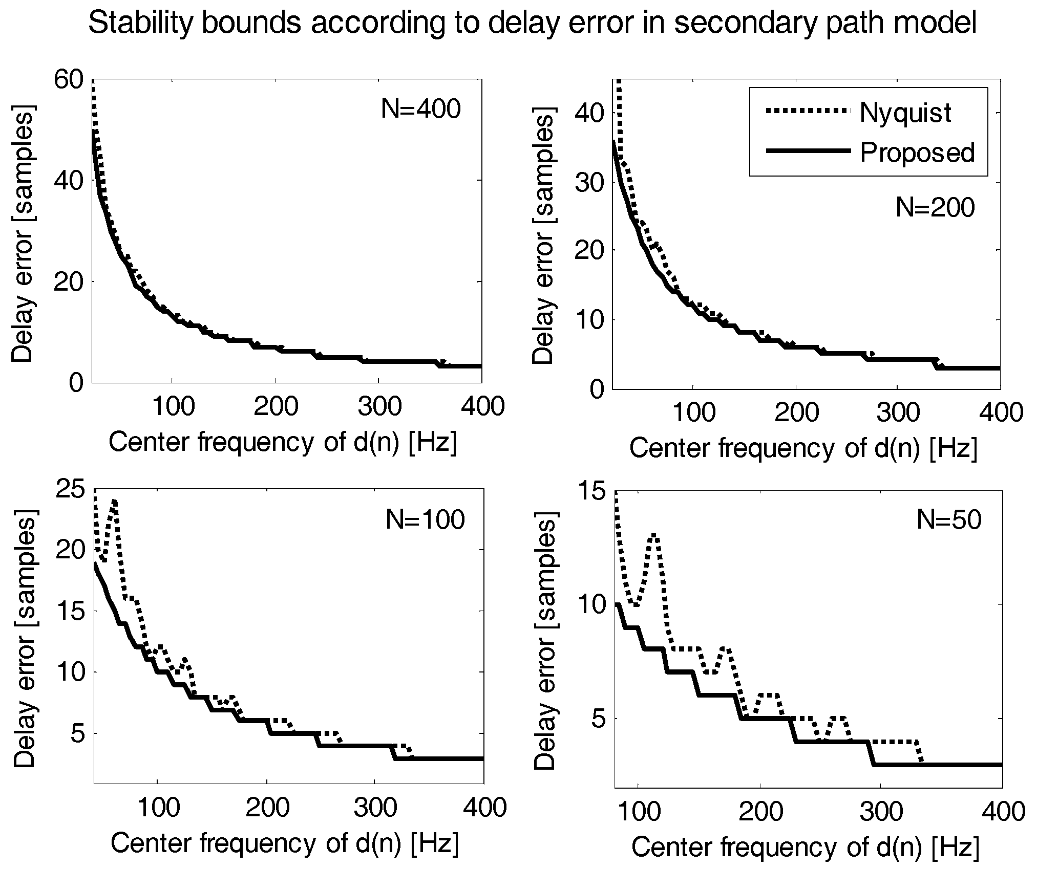
In Figure 6, the stability delay error bounds are obtained with the proposed Equation (23) and compared with the stability bounds obtained with the Nyquist method. The results are obtained for different adaptive filter lengths N = 50, 100, 200 and 400. The proposed stability condition agrees well with the original Nyquist condition showing only few differences in the valid frequency range ${\omega }_0>\pi /N$, i.e., above 80 Hz for N = 100, and above 160 Hz for N = 50.

The bounds of the Nyquist stability condition are obtained by the trial and error method. Many frequency response plots of $W(z)[z^{-\Delta }-z^{-\widehat{\Delta }}]$ are drawn repeatedly on the complex-plane by computer calculation until one of the plots encloses the Nyquist point (−1, 0). The complex plots were drawn for various delay errors in secondary path model and various adaptive filter responses for different lengths of adaptive filter and frequencies of primary noises.

As shown in Figure 6, the proposed results do not exceed the Nyquist results, though the proposed equation’s results give tighter bounds than the bounds of original Nyquist stability condition. For the cases of N = 50 and 100, the large differences below the valid frequency range ${\omega }_0>\pi /N$ are caused by overlapping of the two main lobes of the digital filter responses, which are shown as main two terms in Equation (8).

Simulations are performed with the feedback ANC algorithm based on the filtered-x LMS (FxLMS). Sampling frequency is set to 8 kHz. Delay length of secondary path is set to 10 ms, which is 80 samples in the corresponding sampling frequency. The ANC filter length is set to 200 taps. The tested primary noises are single-tone sinusoidal noises whose frequencies are 50–400 Hz. The normalized least mean square (nLMS) algorithm [18] is used to update the adaptive filter W(z).

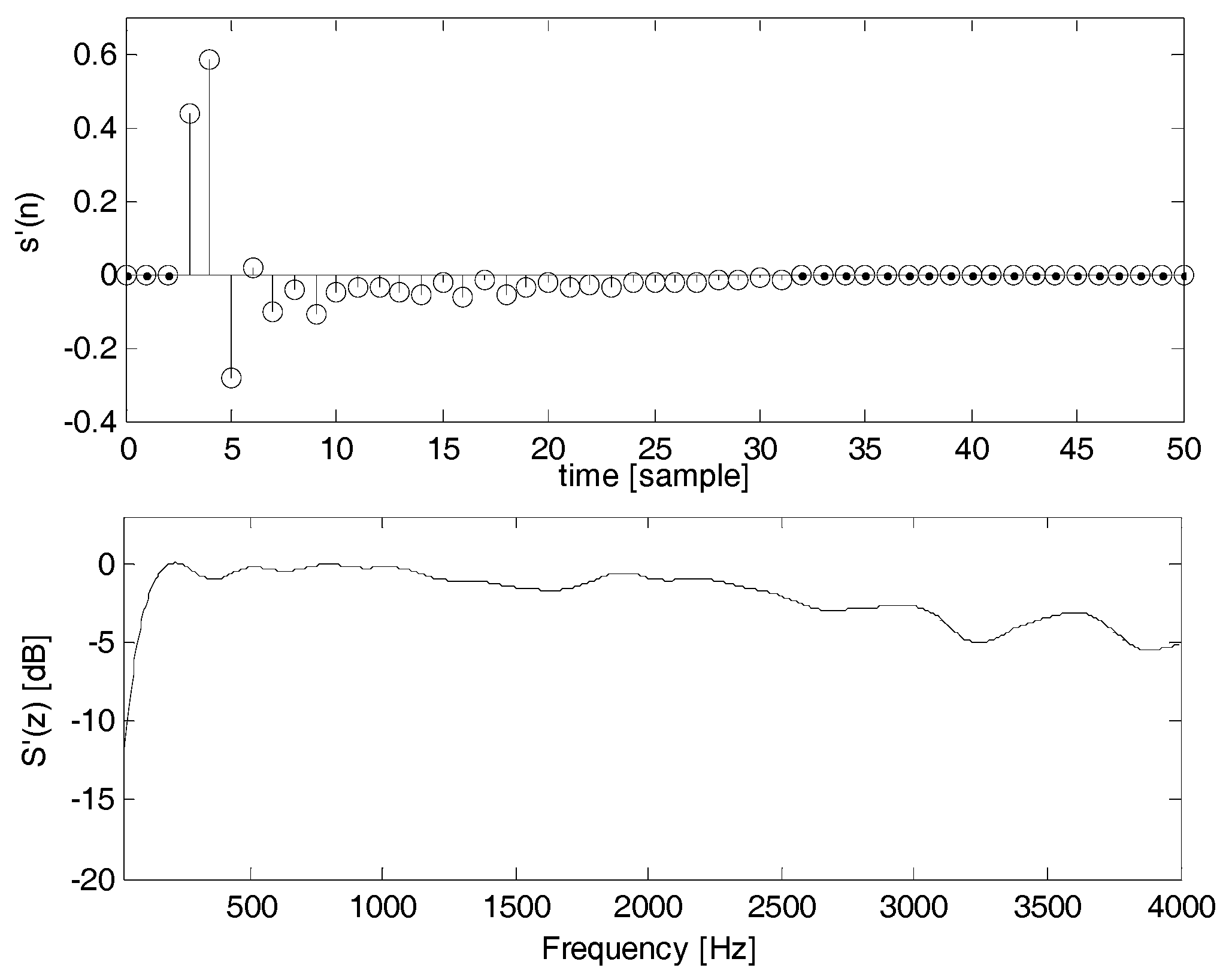
To verify the usage of pure delay model in the proposed analysis, simulations are performed for both cases of pure delay secondary path model and practical secondary path model having delay and spectral distortion. For the practical secondary path model and its estimated model, a spectral distortion component is measured from commercial reference quality headphones and applied to a pure delay model as $S(z)=S’(z)z^{-\Delta }$. For the simulation of various delay error of secondary path model, pure delays around 80 samples are additionally inserted to the measured impulse response, which originally includes 4-sample delay caused by the acoustic propagation between the headphone speaker and the error microphone and the AD/DA converting processing. Figure 7 shows the measured impulse response s’(n) and its frequency response S’(z).

In the frequency response in Figure 7, the roll-off distortion shown in sub bass frequency range lower than 100 Hz is mostly caused by the physical characteristic of the headphone’s speaker and the resonance of the cavity in the headphone ear-cup. Except for the low frequency roll-off, the commercial headphones provide moderate frequency response in most of the ANC system’s operation frequency range.

Simulation is conducted for different number of the adaptive filter lengths and the results are shown in

Table 1. The Stability Bounds of Delay error obtained for different number of adaptive filter taps.

Stability Criterions/Simulations	Number of Adaptive Filter Taps N
	50	100	200	400	600
Nyquist Stability Criterion	8 (1.00 ms)	8 (1.00 ms)	8 (1.00 ms)	9 (1.125 ms)	9 (1.125 ms)
Proposed Equation	6 (0.750 ms)	7 (0.875 ms)	8 (1.00 ms)	9 (1.125 ms)	9 (1.125 ms)
Simulation w/Pure Delay Model	7 (0.875 ms)	8 (1.00 ms)	8 (1.00 ms)	9 (1.125 ms)	9 (1.125 ms)
Simulation w/Measured Response	7 (0.875 ms)	8 (1.00 ms)	8 (1.00 ms)	9 (1.125 ms)	9 (1.125 ms)

* Frequency of primary noise $f_0$ = 150 Hz.

. Frequency of primary noise is set to 150 Hz. For the cases of the filter numbers larger than 100 taps, each bound obtained from the proposed equation and simulation exactly agrees with the original Nyquist results. The large differences of simulation results shown for cases of N = 50 and 100 appear, because the two main lobes of the digital filter responses are wide as much as they are overlapped. There is an inverse relationship between the width of main lobes of the adaptive filter and the tap length of the filter. When the filter length is larger than 200, stability bounds of delay error are obtained as 8 samples for all cases which correspond to 1.00 ms.

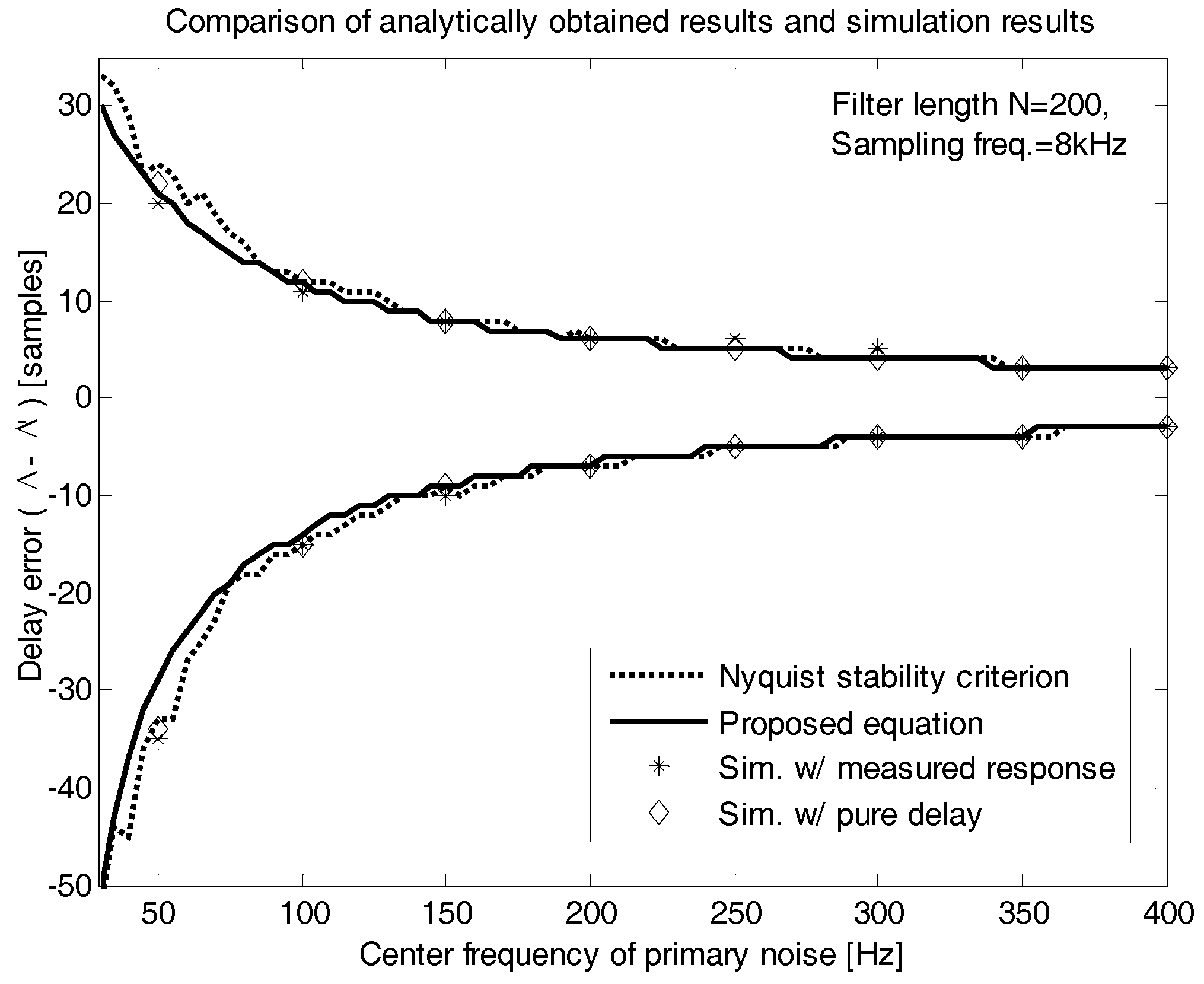
Simulation is also conducted for various frequency of primary noise, and the results are shown and compared to the analytic results in Figure 8. The simulation results of pure delay secondary path model exist between the bounds of Nyquist criterion and those of the proposed method. The simulation results agree well with both the original Nyquist condition and the proposed stability bounds, and show few differences less than 0.250 ms; equivalently, 2 samples for the primary noises have frequencies over 100 Hz. This confirms that the obtained closed-form stability bound Equation (23) is valid. For the case of $\Delta >\widehat{\Delta }$ in Figure 8, the two simulation results from measured secondary path are plotted below the bound of the proposed equation at the noise frequency 50 Hz and 100 Hz. Such result seems due to the low frequency roll-off distortion of the measured secondary path.

6. Conclusions

In this paper, the stability bound of feedback ANC was obtained as a form of a closed-form equation including physical domain design parameters such as noise frequency, length of the adaptive filter, and the mismatch of the secondary path estimation. The performed analysis and the obtained equation not only provide the direct calculation of the stability bound among the design parameters, but they also provide a clear understanding of the behavior of the adaptive filter response and the secondary path modeling error term on the feedback ANC system. Since the stability depends on how much the product of the adaptive filter response term and secondary path error term is close to Nyquist point (−1, 0), the wide band adaptive filter response due to the short filter length and the wide bandwidth of the target noise or spectral distortion of the filter response can cause the stability bound of the feedback ANC to become narrower than the bound of the case of pure delay secondary path model, pure tone primary noise. In the ideal condition of the pure delay secondary path model, the pure tone primary noise, and the infinite adaptive filter length, the stability error bound converges to $\pi /3$ phase difference of the secondary path model. Although some approximations of the formula were used in the derivation process, the analysis result does not violate the original Nyquist stability condition. The performed analysis was verified by conducting simulations for both a pure delay secondary path model and a practical secondary path model. From the simulation results, when tested above 100 Hz primary noise frequency with the filter length N = 200, it is shown that the stability bound of the proposed equation agrees well with both the original Nyquist condition and the simulation results showing less than 0.250 ms difference. Such a closed-form, equation-based stability analysis can provide direct and fast computation of the parameter bounds for stability, so that it is expected to be very useful for the design and real-time operation of the feedback ANC system.