Article

Estimating Underwater Light Regime under Spatially Heterogeneous Sea Ice in the Arctic

1
Takuvik Joint International Laboratory (UMI 3376) Université Laval (Canada) Centre National de la Recherche Scientifique (France), Québec, QC G1V 0A6, Canada
2
Laboratoire d’Océanographie de Villefranche, Sorbonne Université, CNRS, LOV, F-06230 Villefranche-sur-Mer, France
*
Author to whom correspondence should be addressed.
Appl. Sci. 2018, 8(12), 2693; https://doi.org/10.3390/app8122693
Submission received: 8 September 2018 / Revised: 20 November 2018 / Accepted: 23 November 2018 / Published: 19 December 2018
(This article belongs to the Special Issue Outstanding Topics in Ocean Optics)

Abstract

:
The vertical diffuse attenuation coefficient for downward plane irradiance ( K d ) is an apparent optical property commonly used in primary production models to propagate incident solar radiation in the water column. In open water, estimating K d is relatively straightforward when a vertical profile of measurements of downward irradiance, E d , is available. In the Arctic, the ice pack is characterized by a complex mosaic composed of sea ice with snow, ridges, melt ponds, and leads. Due to the resulting spatially heterogeneous light field in the top meters of the water column, it is difficult to measure at single-point locations meaningful K d values that allow predicting average irradiance at any depth. The main objective of this work is to propose a new method to estimate average irradiance over large spatially heterogeneous area as it would be seen by drifting phytoplankton. Using both in situ data and 3D Monte Carlo numerical simulations of radiative transfer, we show that (1) the large-area average vertical profile of downward irradiance, E d ¯ ( z ) , under heterogeneous sea ice cover can be represented by a single-term exponential function and (2) the vertical attenuation coefficient for upward radiance ( K L u ), which is up to two times less influenced by a heterogeneous incident light field than K d in the vicinity of a melt pond, can be used as a proxy to estimate E d ¯ ( z ) in the water column.

1. Introduction

The vertical distribution of underwater light is an important driver of many aquatic processes such as primary production by phytoplankton, and photochemical reactions such as the photodegradation of organic matter. Hence, an adequate description of the underwater light regime is mandatory to understand energy fluxes in aquatic ecosystems. In open water, when assuming an optically homogeneous water column, downward irradiance at any given wavelength follows, as a first approximation, quite well a monotonically exponential decrease with depth, which can be modelled as follows [1] (Equation (1)):
E d ( z ) = E d ( 0 ) e K d ( z ) z
where E d ( z ) is the downward plane irradiance (W m 2 ) at depth z (m), E d ( 0 ) is the downward plane irradiance (W m 2 ) just below the surface and K d ( z ) is the diffuse vertical attenuation coefficient (m 1 ) describing the rate at which downward irradiance decreases with increasing depth. K d is one of the most commonly used apparent optical properties (AOP) of seawater, and a good estimation of this parameter is important for measuring or modelling primary production. K d may vary with depth because of changes in seawater inherent optical properties (IOPs), the angular structure of the light field, and the effects of inelastic radiative processes such as Raman scattering by water molecules and fluorescence by phytoplankton pigments or dissolved organic matter. As Kirk [1] pointed out, for practical considerations in oceanography and limnology, the K d value, even when averaged within the euphotic zone, provides a useful proxy to represent the downward irradiance attenuation in the upper water column. For example, to determine primary production based on simulated on-deck incubations or photosynthetic parameters derived from photosynthesis–irradiance curves (P vs. E curves) requires measured or estimated values of K d (e.g., Morel [2]). Nowadays, K d is relatively easy to estimate using commercially available radiometers.
The ice-infested regions of the Arctic ocean are characterized by a complex mosaic made of sea ice with snow, melt ponds, ridges, and leads [3,4,5]. Phytoplankton are exposed to a highly variable light regime while drifting under these heterogeneous features (e.g., Lange et al. [6]). Estimating primary production of phytoplankton under sea ice requires an approach that is adequate to capture this large-area variability in the light field. In situ incubations at single locations of seawater samples inoculated with 14 C or 13 C are not appropriate because they reflect primary production under local light conditions, which is not representative of the range of irradiance experienced by drifting phytoplankton over a large area. One classical approach that is more adequate consists in conducting on-deck simulated 24-h incubations of seawater samples inoculated with 14 C or 13 C and applying the light attenuation at the depths of sample collections, using natural illumination and neutral filters. An alternative approach consists in calculating primary production using modelled or measured daily time series of incident irradiance, sea ice transmittance and in-water vertical attenuation coefficients, combined with photosynthetic parameters determined from P–E curves measured with short (under two hours) incubations of seawater samples inoculated with 14 C. The latter two methods require that the vertical profile of the irradiance experienced by drifting phytoplankton be appropriately determined, which is challenging due to surface heterogeneity. Traditionally, one or very few E d ( z ) profiles are measured at discrete locations under sea ice (e.g., Mundy et al. [7]). Such measurements, however, do not capture the variability induced by sea ice features. In recent studies, to better document the spatial variability of E d ( z ) , radiometers were attached to either remotely operated vehicles (ROV) [4] or a surface and under-ice trawl (SUIT), a net developed for deployment in ice-covered waters, typically behind an icebreaker [6]. Both a ROV and a SUIT allow a better description of the light field right under sea ice, which is more appropriate for determining average irradiance experienced by drifting phytoplankton. Such under-ice measurements can then be combined with averaged K d values to propagate light at depth.
Estimating irradiance at depth for primary production measurement or calculation using K d values derived from only a few discrete vertical profiles of E d ( z ) under heterogeneous sea ice is problematic whatever the platform for radiometer deployment. Let us consider that phytoplankton, by continuously drifting horizontally relative to sea ice, are exposed to fluctuations in irradiance due to surface heterogeneity, and that the relevant light metrics for primary production in such conditions is irradiance at any depth averaged over some horizontal area. When measuring an irradiance profile at one given location under sea ice, as the depth of the upward-looking detector increases, light from a larger area on the underside of the ice enters the detector field of view. In other words, the detector “sees” different things at different depths. One consequence is that E d ( z ) measured that way may not follow the usual monotonically exponential decrease with increasing depth (Equation (1)). For example, irradiance profiles measured beneath low-transmission sea ice (e.g., white ice) relative to surrounding areas showing melt ponds, show subsurface light maxima. The literature reports subsurface maxima varying between 5 m and 15 m in depth [5,8,9]. Conversely, it is also important to note that K d estimations are biased when profiles are measured beneath an area of high transmission (e.g., a melt pond) relative to surrounding areas [5]. Indeed, with depth, light decreases more quickly than what would be expected from the IOPs of the water column. In the field, this situation is more difficult to identify compared to profiles showing subsurface maxima because the former measurements may appear to follow a single exponential decrease but would not produce a diffuse attenuation coefficient that adequately describes the water mass. So, two vertical light profiles measured a few meters apart under sea ice are often very different. More importantly, local measurements of light under heterogeneous sea ice do not provide an adequate description of the average light field as it would be seen by drifting phytoplankton cells at different depths. This makes estimations of primary production and the interpretation of biogeochemical data challenging in the presence of sea ice.
To fit vertical profiles of E d ( z ) under bare ice that do not follow an exponential decay under sea ice covered with melt ponds, Frey et al. [8] proposes a simple geometric model (Equation (2)).
E d ( z ) = π E d ( 0 ) ( 1 + P ( N 1 ) cos 2 ϕ ) e K d ( z ) z
where E d ( 0 ) is the irradiance directly below the ice/snow, P the areal fraction of the ice cover, N the ratio between ice and melt ponds transmittance and ϕ a fitting parameter defined as arctan ( R / z ) with R the radius of the ice patch and z the depth. A major drawback of this method is that additional field observations of N and P are required to adequately parametrise the model, which makes its use more difficult. To address this concern (among others), Laney et al. [9] proposed a semi-empirical parametrisation that includes a second exponential coefficient in Equation (1) to model light decrease at the interface between the ice and ocean water at the bottom of the ice layer (Equation (3)):
E d ( z ) = E d ( 0 ) e K d ( z ) z ( E d ( 0 ) E d ( NS ) ) e K N S ( z ) z
where E d ( 0 ) is the irradiance that would be observed under homogeneous snow or ice cover, E d ( NS ) is the irradiance under-ice, and K N S ( z ) describes the decrease of E d ( 0 ) just under the ice layer. Both the methods by Frey et al. [8] and Laney et al. [9] make it possible to propagate local E d ( z ) vertically under low transmission ice. However, these methods cannot identify and correct for inflated K d when profiles are measured beneath an area of high transmission relative to surrounding areas. Additionally, when trying to determine primary production by phytoplankton that drift under sea ice and therefore are not static under sea ice features, what matters is the average shape of the vertical E d ( z ) profile, which may possibly be predictable using a large-area K d ¯ as under a wavy open ocean surface [10].
In this study, using both in situ data and 3D Monte Carlo numerical simulations of radiative transfer, we show that the vertical propagation of average E d ( z ) , E d ¯ ( z ) , is reasonably well approximated by a single exponential decay with a so-called large area K d , K d ¯ , under sea ice covered in melt ponds. We further demonstrate that K d ¯ can be estimated from the vertical attenuation coefficient for upward radiance ( K L u ) because the latter is apparently less affected by local surface features of the ice cover. We implicitly assume that primary production can be adequately modelled using E d ¯ ( z ) , and we conclude that K L u is an appropriate AOP for predicting the vertical variations in E d ¯ ( z ) under sea ice.

2. Material and Methods

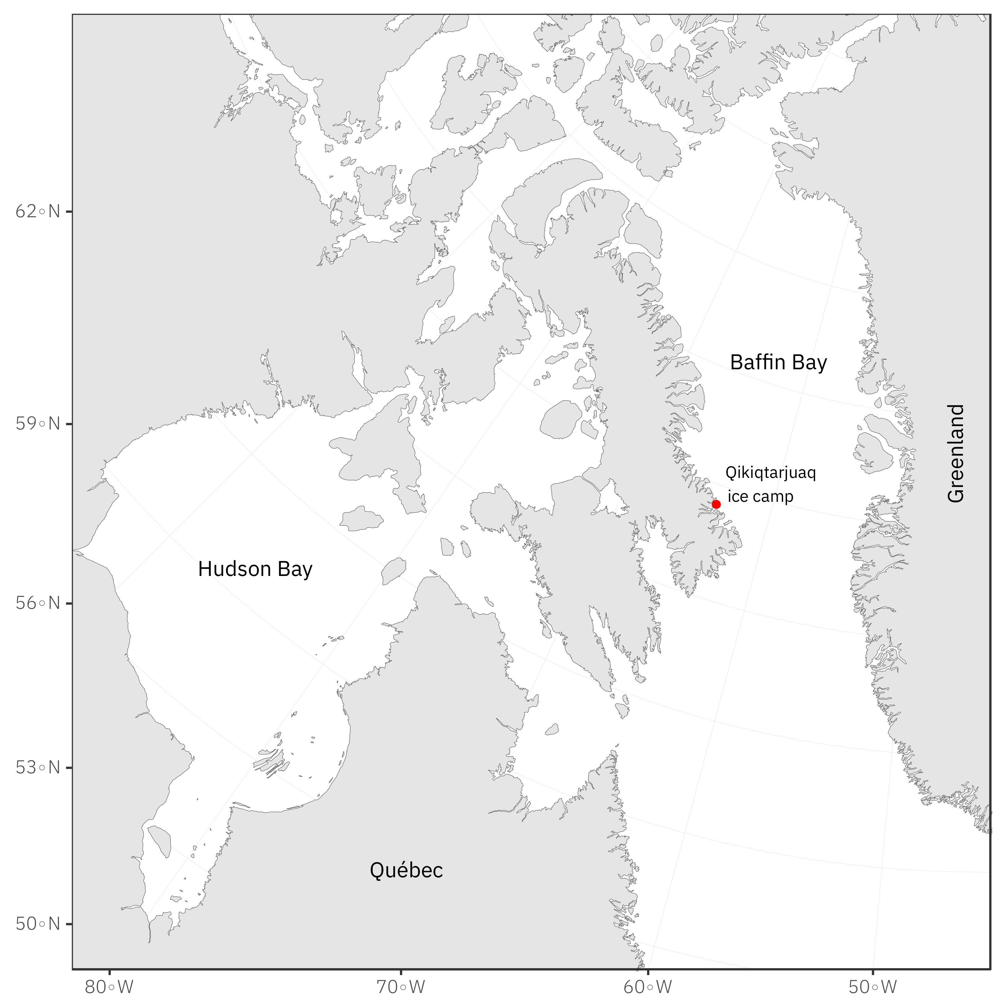
2.1. Study Site and Field Campaign

The field campaign was part of the GreenEdge project (www.greenedgeproject.info) which was conducted on landfast ice southeast of the Qikiqtarjuaq Island in the Baffin Bay (67.4797 N, 63.7895 W). The field operations took place at an ice camp where the water depth was 360 m, from 20 April to 27 July 2016 (Figure A1 included in Appendix A). During the sampling period, the study site experienced changes in the snow cover and landfast ice thickness of 0–49 cm and 106–149 cm, respectively.

2.2. In Situ Underwater Light Measurements

During the campaign, a total of 83 vertical light profiles were acquired using a factory-calibrated ICE-Pro (an ice floe version of the C-OPS, or Compact-Optical Profiling System, from Biospherical Instruments Inc., San Diego, CA, USA) equipped with both downward plane irradiance E d ( z ) (W m 2 ) and upward radiance L u ( z ) (W m 2 sr 1 ) radiometers. The ICE-Pro system is a negatively buoyant instrument with a cylindrical shape 10 inches in diameter and is not designed for free-fall casts (as opposed to its open-water version). To perform the profiles, the frame was manually lowered into an auger hole that had been cleaned of ice chunks. Once it was underneath the ice layer, fresh clean snow was shovelled back in the hole to prevent the creation of a bright spot right on top of the sensors. Great care was taken not to pollute the hole surroundings (footsteps, water and slush spillage from the auger drilling, etc.). The operator then stepped back 50 m, while keeping the sensors right under the ice, to avoid any human shadow on top of the profile. The frame was then lowered manually at a constant descent rate of approximately 0.3 m s−1. The above-surface atmospheric reference sensor was fixed on a steady tripod standing on the floe approximately 2 m above the surface and above all neighbouring ice camp features. Data processing and validation were performed using a protocol inspired by the one proposed by Smith and Baker [11]. Measurements were made at 19 wavelengths: 380, 395, 412, 443, 465, 490, 510, 532, 555, 560, 589, 625, 665, 683, 694, 710, 765, 780 and 875 nm. For this study, E d and L u spectra were interpolated linearly between 400 and 700 nm every 10 nm. In situ diffuse attenuation coefficients (K) for both E d ( K d ) and L u ( K L u ) were calculated on a 5 m sliding window (10–15 m, 15–20 m, , 70–75 m, 75–80 m) starting at 10 m depth to reduce the effects of surface heterogeneity. A total of 72,044 non-linear models were calculated to estimate both K coefficients from Equation (1) (83 profiles × 14 depths × 31 wavelengths × 2 radiometric quantities ( E d , L u )). A conservative R 2 of 0.99 was used essentially to filter out noisy profiles. 42,407 models were kept for subsequent analysis.

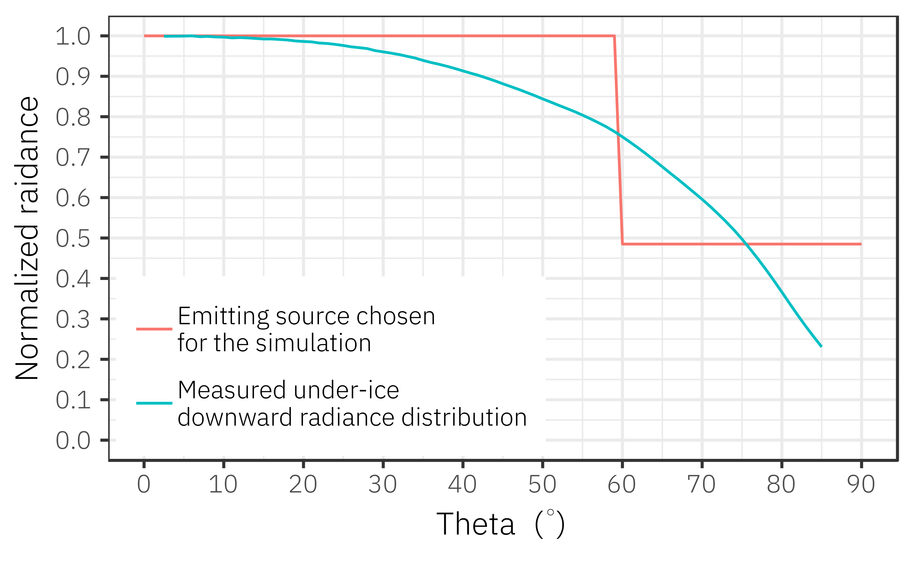
2.3. 3D Monte Carlo Numerical Simulations of Radiative Transfer

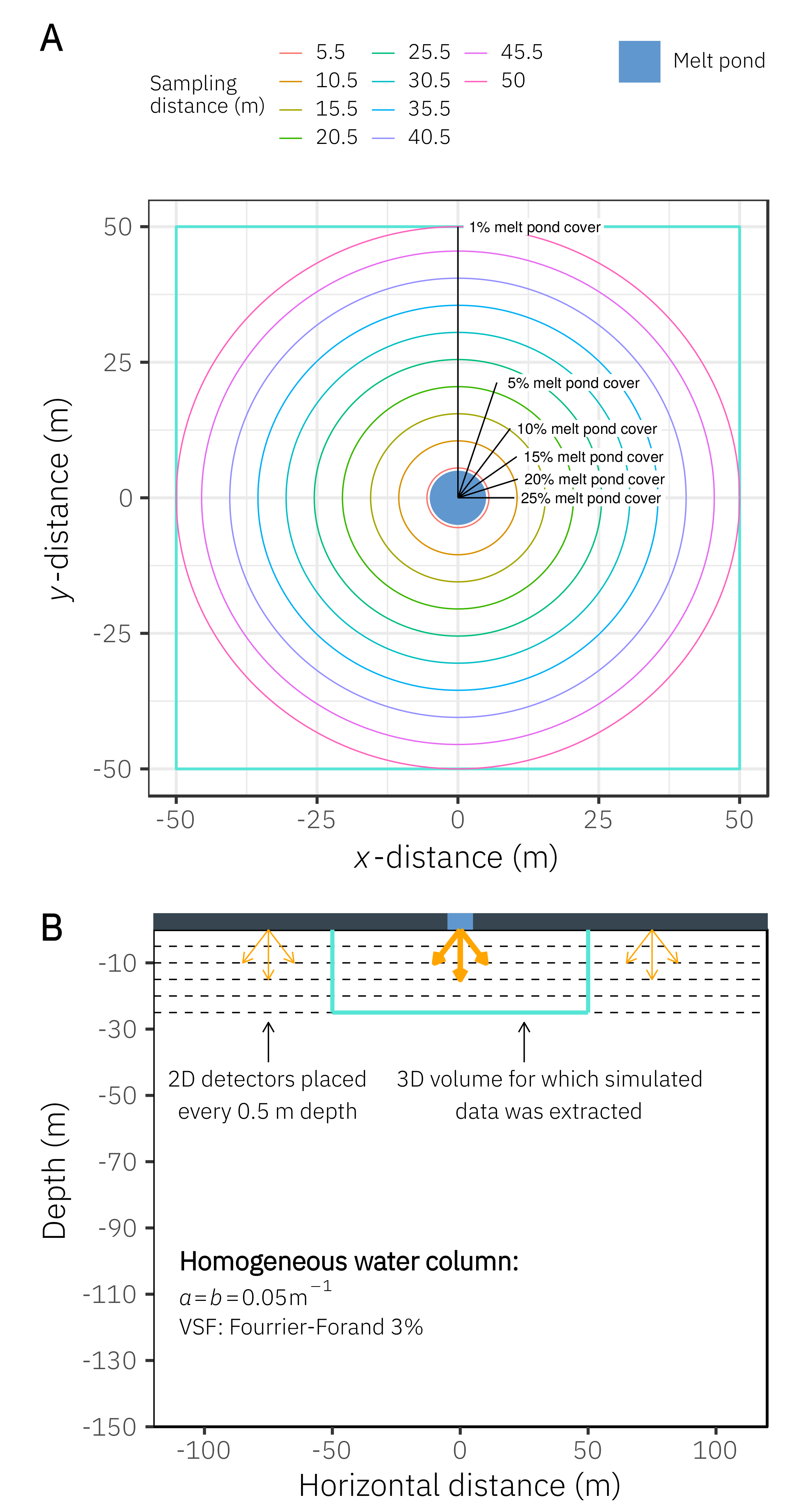
2.3.1. Theory and Geometry

3D numerical Monte Carlo simulation is a convenient approach for modelling the light field under spatially heterogeneous sea surfaces [5,12,13,14]. They are simple to understand and versatile, and incident light, IOPs and geometry can be easily changed. In this study, we used SimulO, a 3D Monte Carlo software program that simulates the propagation of light in optical instruments or in ocean waters [15]. Our objective was to simulate the propagation of sunlight underneath heterogeneous ice-covered ocean waters. Simulations were performed in an idealized ocean described by a cylinder of 120 m radius and 150 m depth (Figure 1). The water IOPs were selected to reflect pre-bloom conditions in the green–blue spectral region ( a = b = 0.05 m 1 ). These typical averaged values were measured during the GreenEdge 2016 campaign using an in situ spectrophotometer (ac-s from Sea-Bird Scientific) and represent the contribution of both pure water and the water constituents. The scattering phase function was described by a Fournier-Forand analytic form with a 3% backscatter fraction [16,17]. The inclusion of a 3D sea ice layer at the upper boundary of the ocean would require extensive computing power because of the high scattering properties of sea ice. Instead, sea ice was incorporated at the upper boundary of the ocean using a 2D light-emitting surface with a radius of 100 m. The angular distribution and magnitude of the light field emitted by the surface was chosen to mimic observed field data [18]. SimulO does not allow the use of arbitrary angular distribution for photon-emitting surfaces. To overcome this problem, two sources of photons were summed up in order to reproduce an observed under-ice light field (Figure 2). The first source was a regular Lambertian emitting surface while the second was a Lambertian emitting surface but restricted to an emission within 60 degrees of the zenith angle. A 5-m radius melt pond was set up at the center of the emitting surface (Figure 1). The melt pond had the same emitting angular distribution as the surrounding ice. Its intensity was four times higher than the surrounding ice, which corresponds to typical conditions found in the Arctic during summer [19].
Given our interest in surface light profiles, 2D horizontal software detectors were placed vertically every 0.5 m, from 0.5 m up to a depth of 25 m. Detectors include 1 m2 pixels measuring downward irradiance and upward radiance (5-degree half angle of acceptance). In order to avoid the effect of the boundary (i.e., absorption by the side of the cylinder used to simulate the water column), data outside a radius of 50 m were not used (see the green box in Figure 1). A total number of 7.14 × 10 10 photons were simulated to obtain a sufficient number of upwelling photons. The simulation took approximately 6000 h distributed over 2000 CPU cores. Because the geometry was symmetrical azimuthally, irradiance and radiance were averaged over the azimuth in order to increase the signal-to-noise ratio. Because of the low scattering coefficients used to reproduce in situ conditions observed during the sampling campaign, radiance profiles were noisy because a small number of upward photons could be captured. To address this issue, radiance profiles were smoothed using a Gaussian fit (Figure A2 included in the Appendix B).

2.3.2. Estimation of Reference and Local Light Profiles

To explore how the melt pond influences the averaged underwater irradiance and radiance profiles (Figure 1), data from the Monte Carlo simulation were averaged according to six different radii, corresponding to varying melt pond spatial proportions. The simulated light profiles were averaged within the following surface areas: (1) 10 m radius (25% melt pond cover), (2) 11.18 m radius (20% melt pond cover), (3) 12.91 m radius (15% melt pond cover), (4) 15.81 m radius (10% melt pond cover), (5) 22.36 m radius (5% melt pond cover) and (6) 50 m radius (1% melt pond cover). For each of these six configurations, the corresponding averaged light profile, E d ¯ ( z ) , was subsequently viewed as an adequate description of the average underwater light field. For the remainder of the text, these averaged profiles are referred to as reference light profiles. Furthermore, 50 light profiles, evenly spaced by 1 m from the melt pond centre, were extracted to mimic local measurements of light and to calculate associated diffuse attenuation coefficients.

2.4. Statistical Analysis

All statistical analyses and graphics were carried out with R 3.5.1 [20].

3. Results

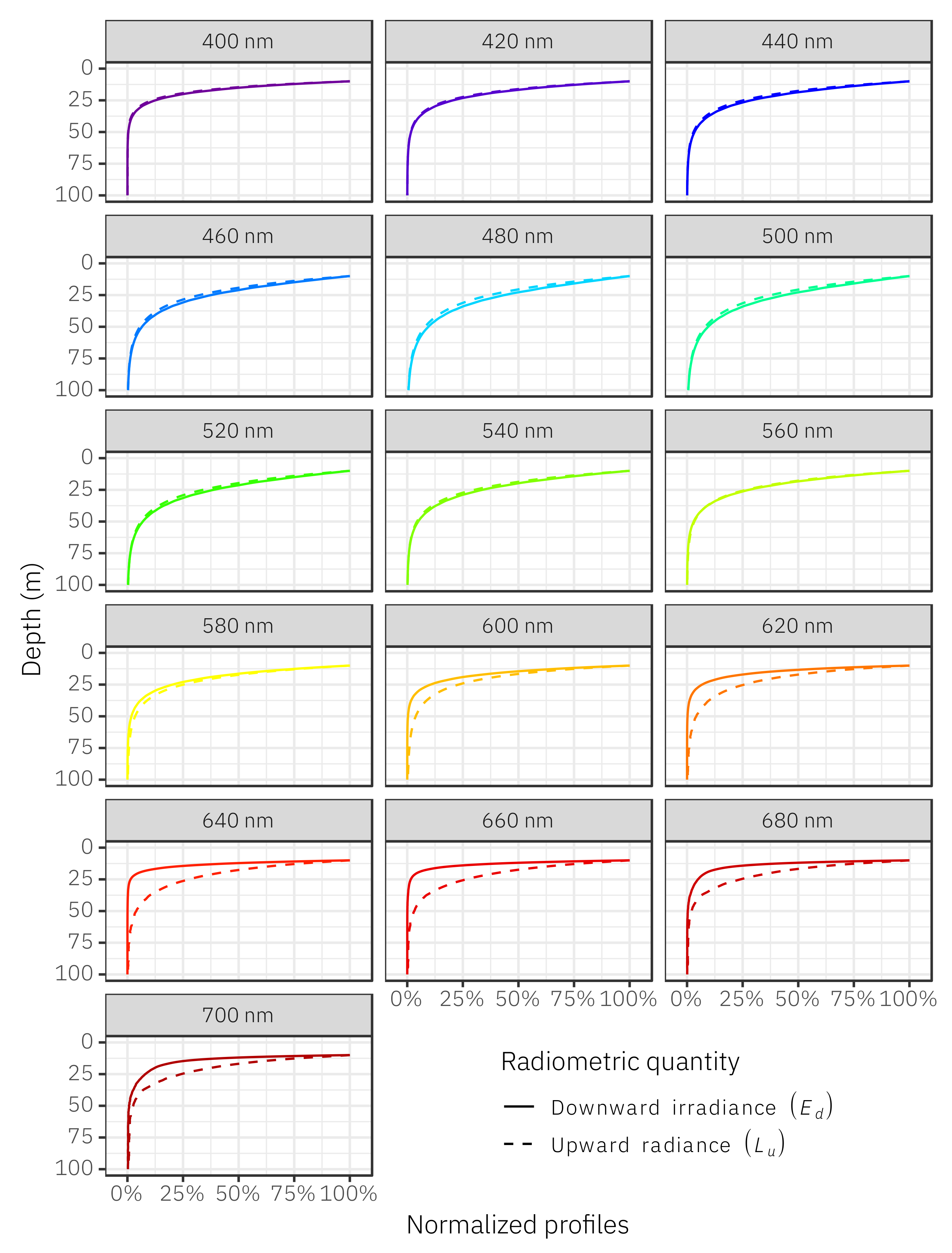
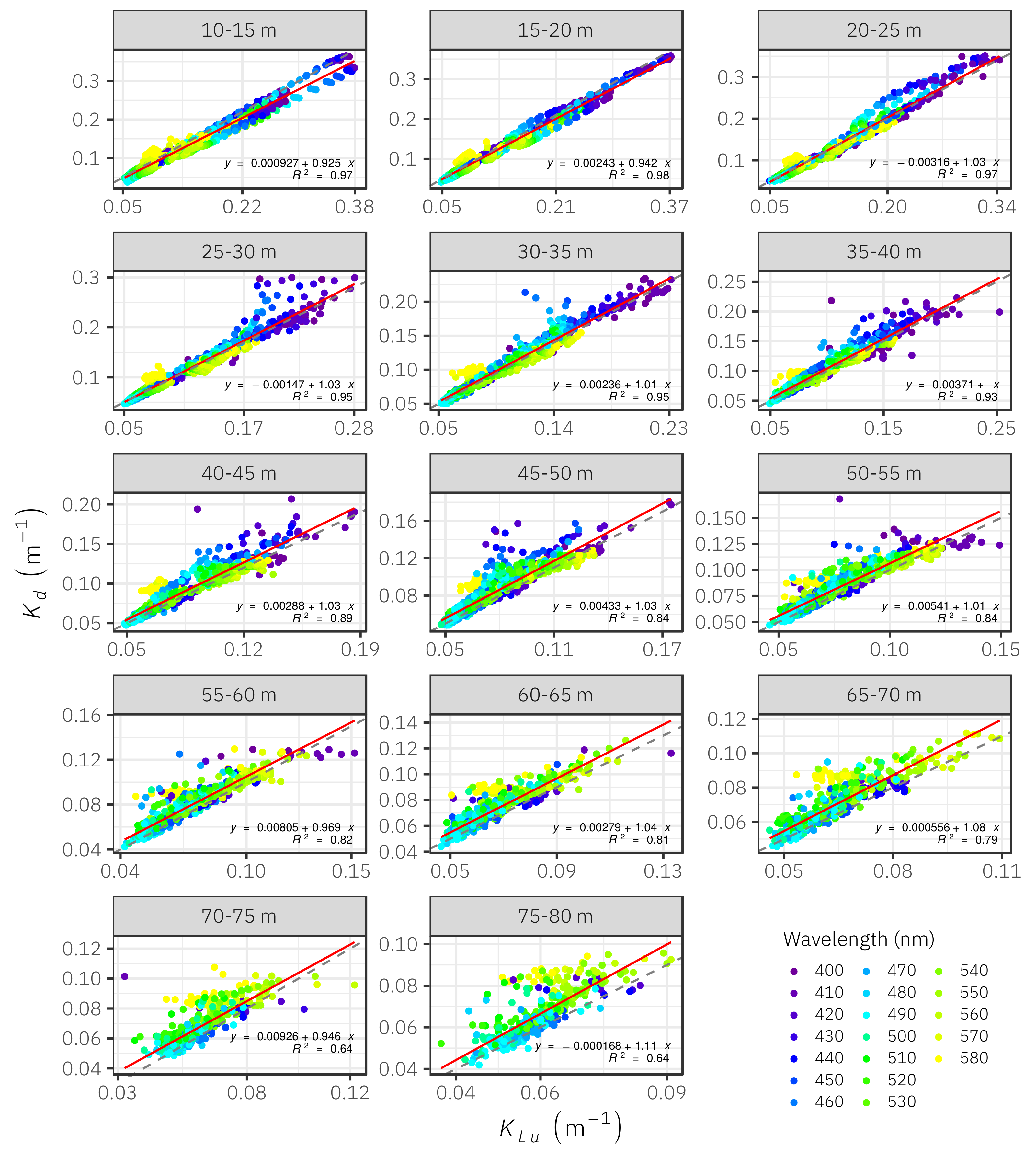
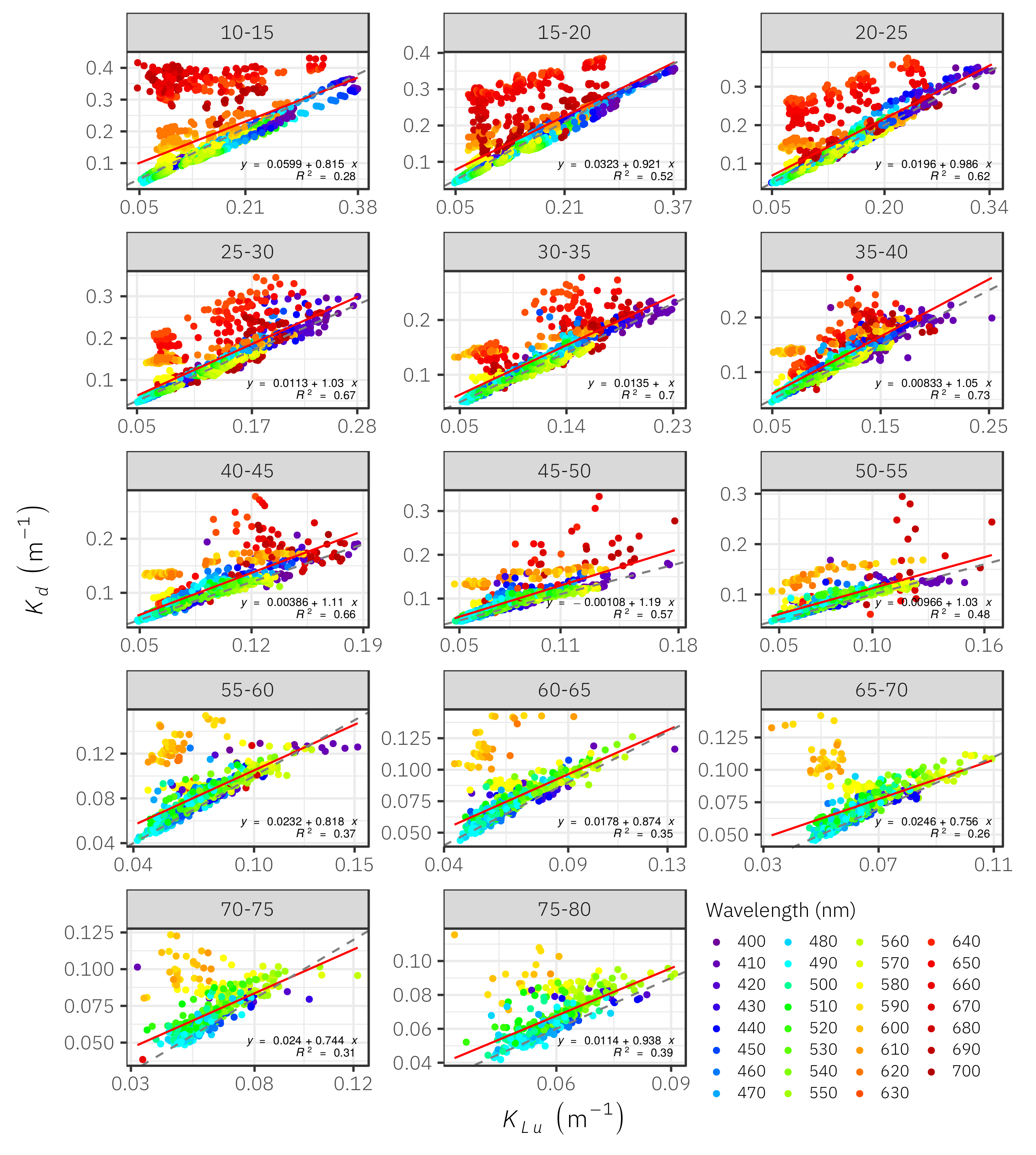
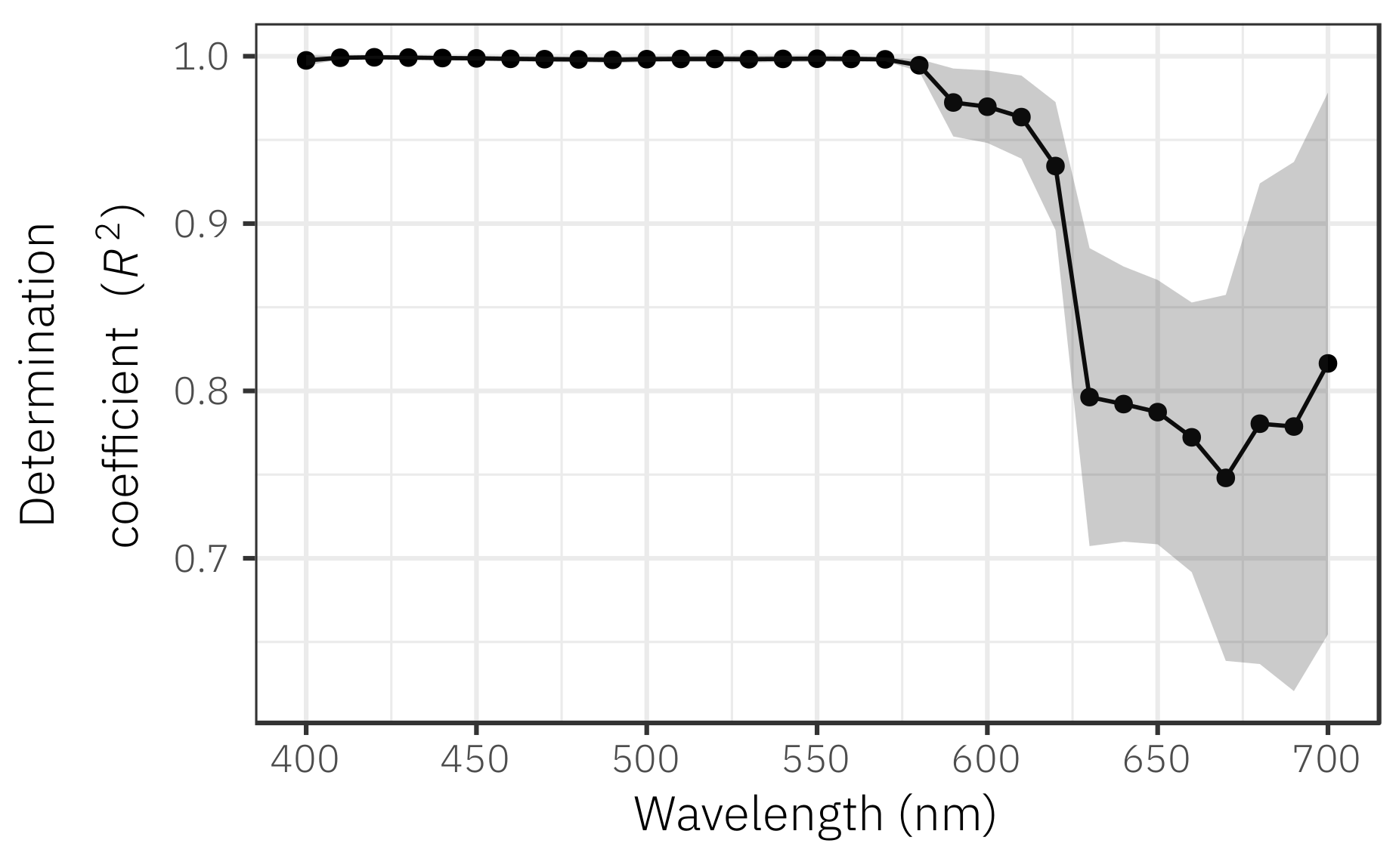
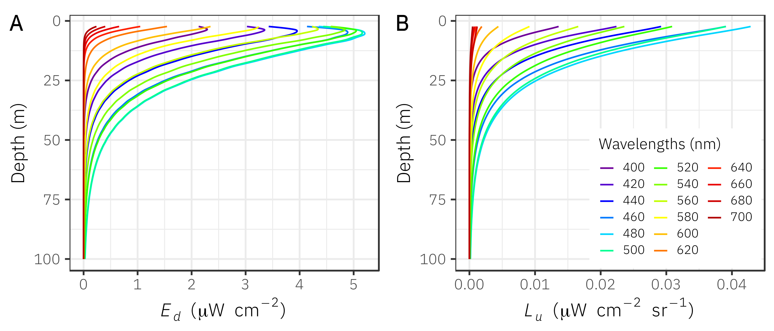
3.1. Comparing In Situ Downward Irradiance ( E d ) and Upward Radiance ( L u ) Measurements

An example showing in situ downward irradiance ( E d ) profiles and upward radiance ( L u ) profiles at 16 visible wavelengths measured under-ice is presented in Figure 3. For the E d profiles, subsurface light maxima at a depth of around 10 m are clearly visible between 400 and 560 nm. These peaks are not visible in the yellow/red region (580–700 nm). For the L u profiles, no subsurface light maxima were found at any wavelength. To have a closer look at the shape of both E d and L u profiles, data below the 10 m depth were normalized to the value at 10 m (Figure 4). Below 10 m and between 400 and 580 nm, both E d and L u profiles presented the same shape (i.e., yield the same rate of attenuation with increasing depth). At longer wavelengths (≥600 nm), differences between the shapes of E d and L u profiles increased. Irradiance and radiance diffuse attenuation coefficients ( K d and K L u ) calculated for the layers of a 5 m thickness are compared in Figure 5 for all 83 profiles. In the blue/green/yellow regions (400–580 nm), the determination coefficients between K L u and K d varied between 0.98 at the surface (10–15 m) and 0.64 at depth (75–80 m). For most of the surface layers, regression lines lined up with the 1:1 lines. Slight deviations from the 1:1 lines started to appear below 60 m where K d was on average higher than K L u . The relationships including orange and red wavelengths are presented in Figure A3 included in the Appendix C. A linear regression analysis between all in situ normalized E d and L u profiles showed that determination coefficients ( R 2 ) range between 0.75 and 1 (Figure A4). A sharp decrease and a high variability of calculated R 2 occurred beyond 575 nm. This suggests a gradual decoupling between E d and L u profiles at longer wavelengths, likely due to the effect of inelastic scattering (mostly Raman scattering).

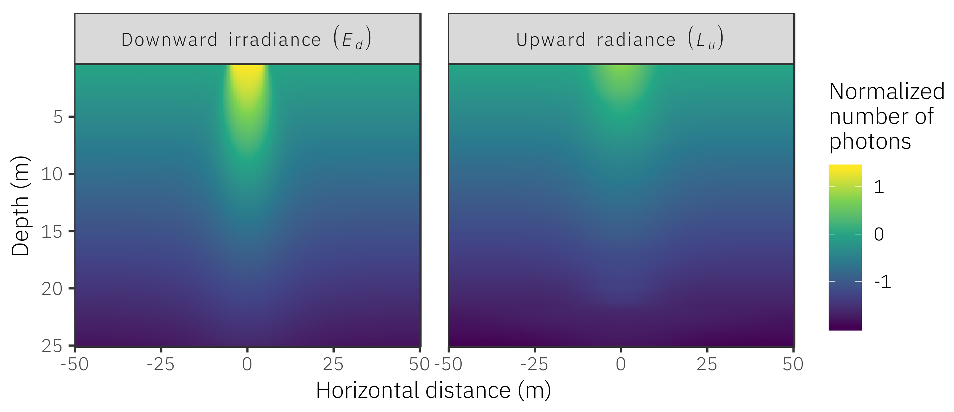
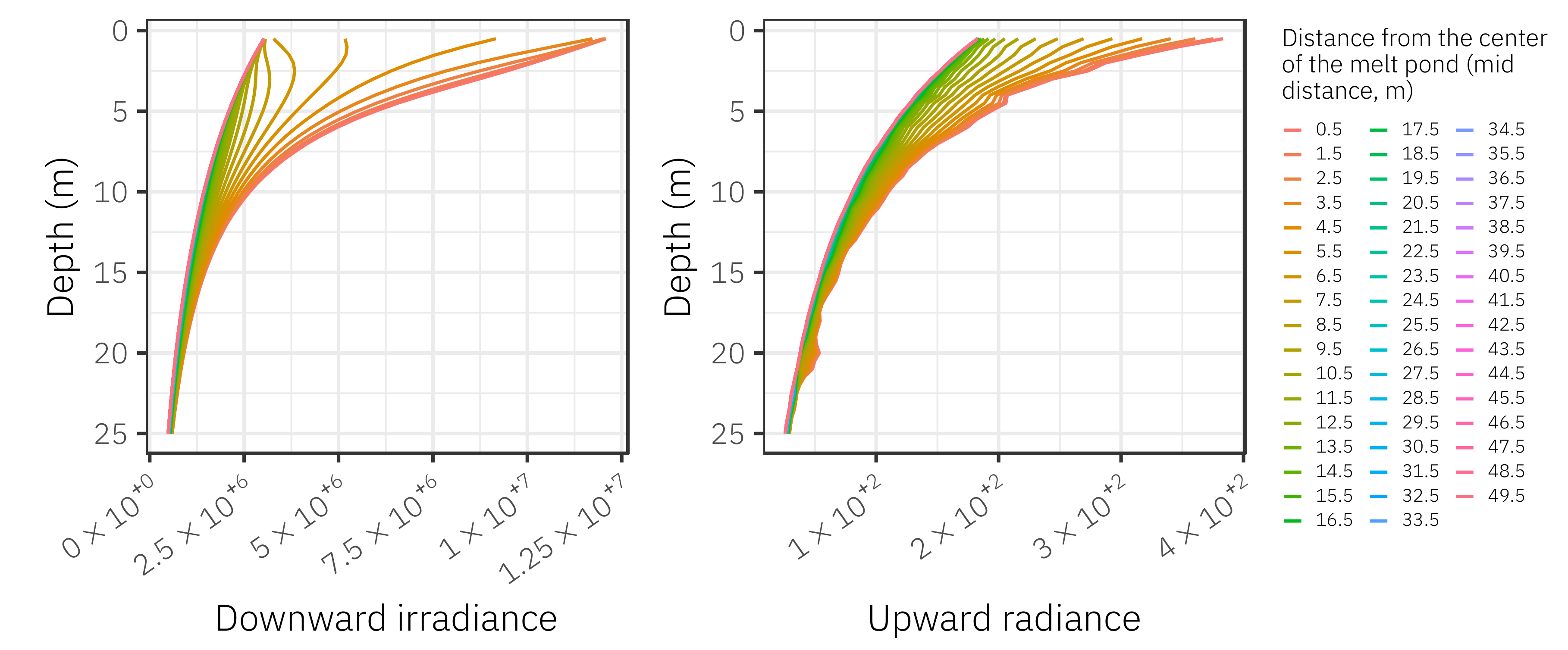
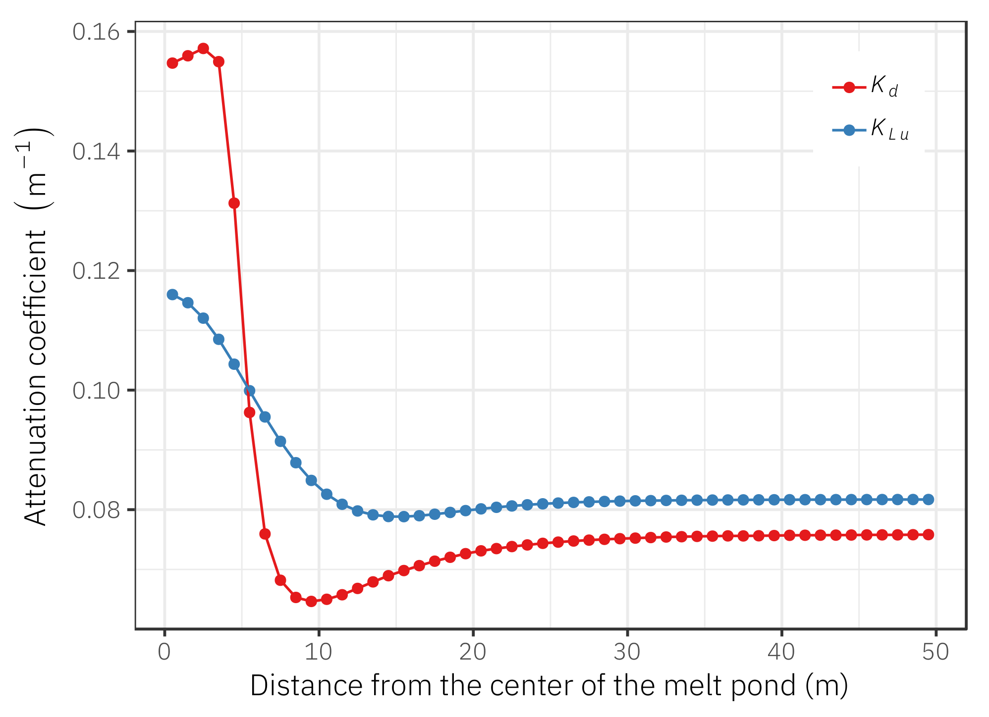
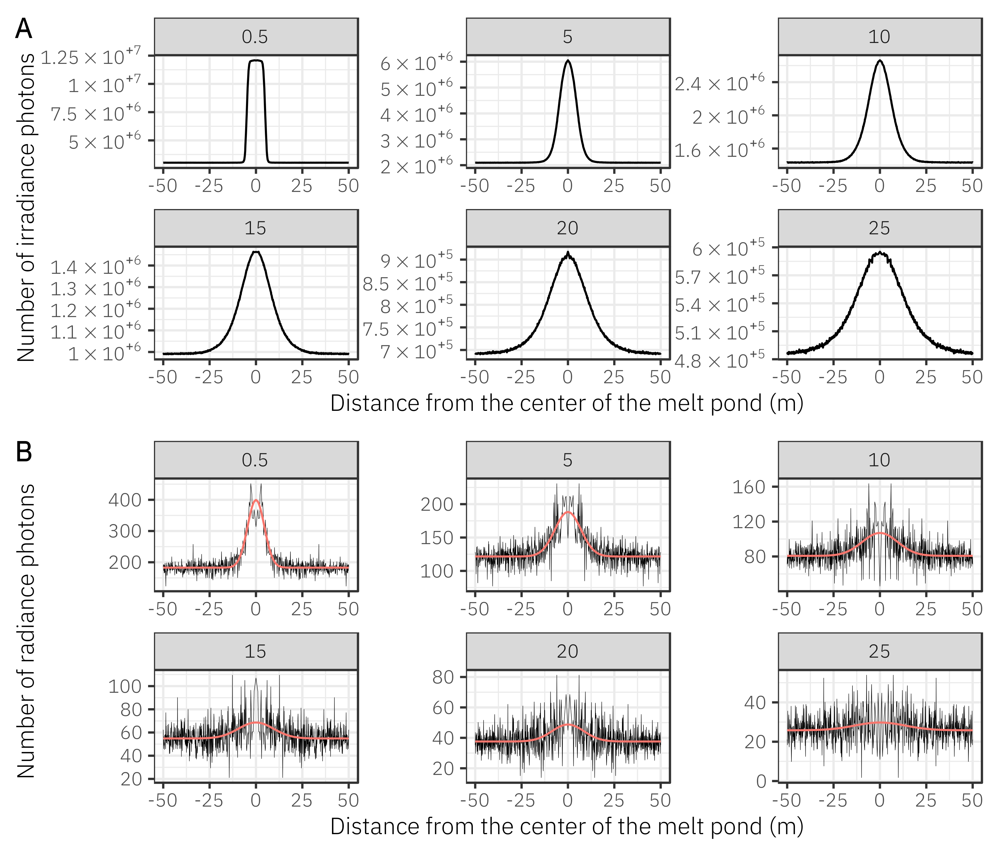
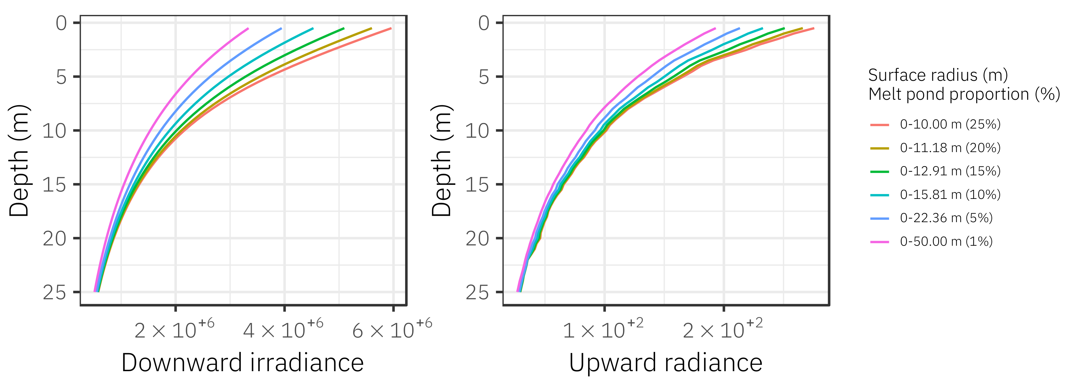
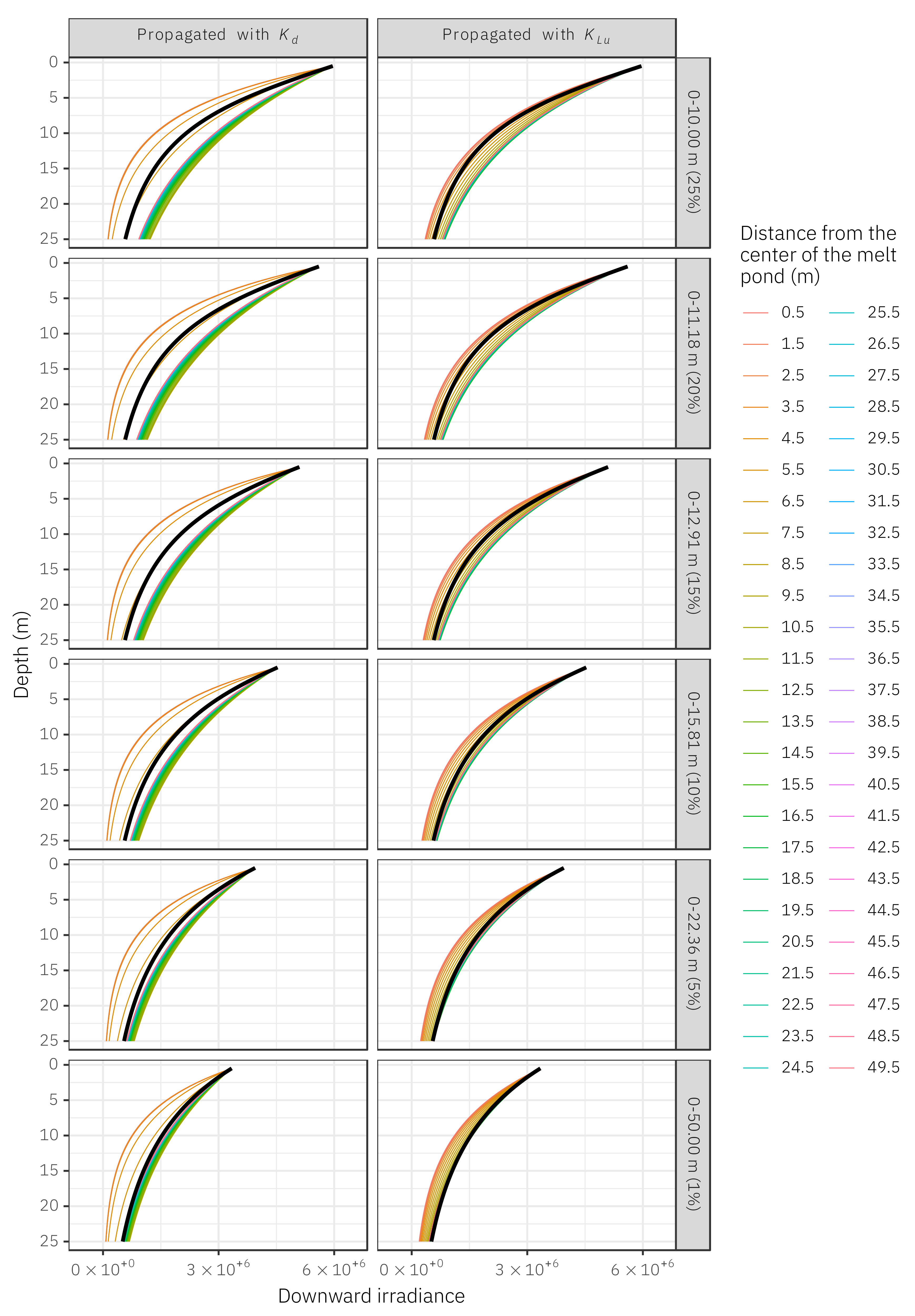
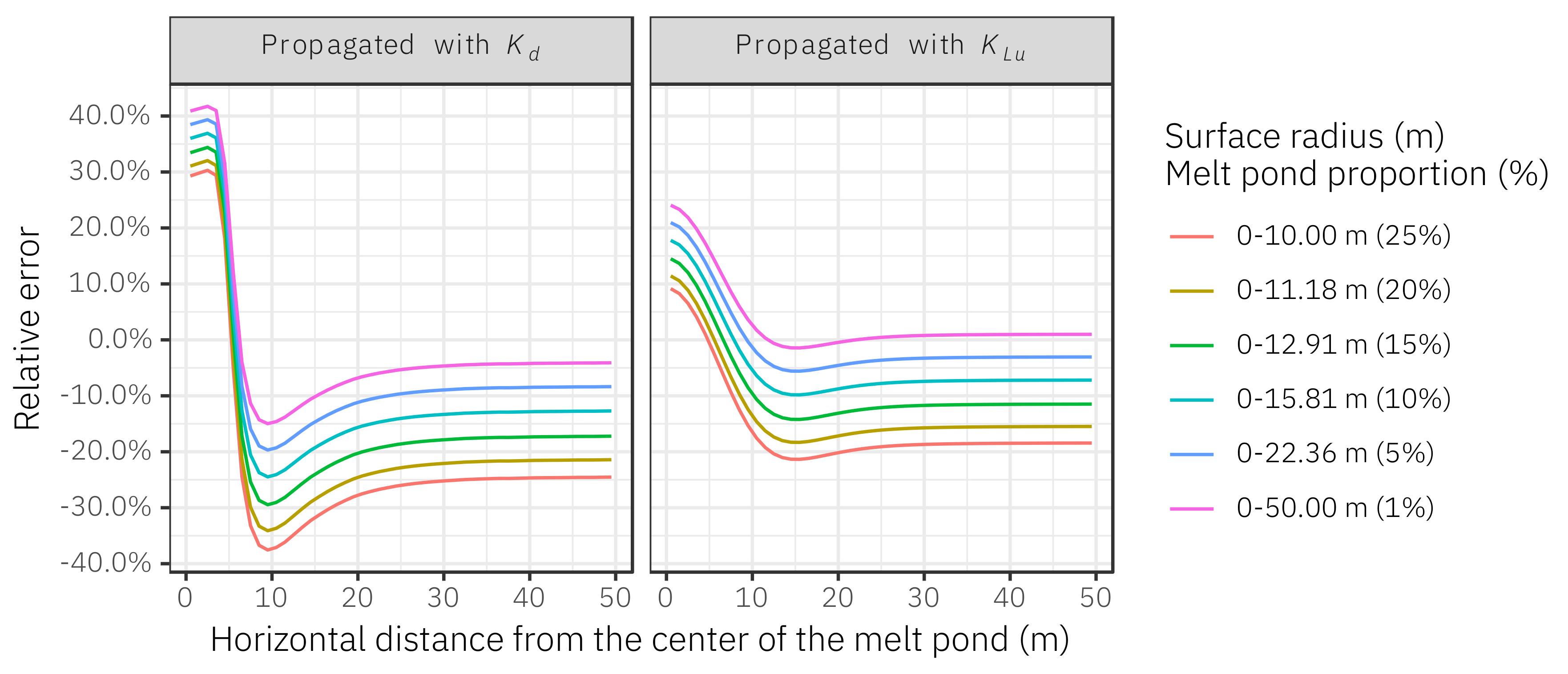
3.2. 3D Monte Carlo Numerical Simulations

Figure 6 shows cross-sections of the simulated downward irradiance and upward radiance. A key difference for the upcoming discussion is that the simulated upward radiance was more homogeneous compared to the simulated downward irradiance. Figure 7 shows the reference irradiance, E d ( z ) , and reference radiance, L u ( z ) , profiles. The highest irradiance and radiance occurred when the melt pond occupied 25% of the sampling area, allowing for more light to propagate in the water column. None of the E d ( z ) and L u ( z ) reference profiles showed subsurface light maxima. Figure 8 shows the 50 simulated local downward irradiance and upward radiance profiles evenly spaced by 1 m in the horizontal distance from the melt pond centrer. Local downward irradiance profiles under the melt pond (0–5 m) showed a rapid decrease with increasing depth described by a monotonically exponential or quasi-exponential decrease. Local simulated downward irradiance profiles just outside the melt pond (5–10 m from the melt pond centre) were characterized with subsurface light maxima occurring at a depth of between approximately 5 and 10 m. Further away from the melt pond centre, downward irradiance profiles followed a monotonically exponential or quasi-exponential decrease. None of the simulated upward radiance profiles presented subsurface light maxima (Figure 8). From local simulated irradiance and radiance profiles (Figure 8), K d and K L u were calculated by fitting Equation (1) between the depths of 0 m and 25 m. Results are presented in Figure 9. K d varied between 0.065 and 0.157 m 1 and K L u between 0.079 and 0.116 m 1 . These K d and K L u were used to propagate light downward from surface reference values E d ( 0 ) . Figure 10 shows the profiles resulting from this calculation. A greater dispersion around the reference profiles (thick black lines in Figure 10) occurred when using K d compared to the profiles generated with similarly derived K L u values. The relative differences between the depth-integrated values of each local profile (coloured lines in Figure 10) and the depth-integrated values of the reference profiles (thick black lines in Figure 10) were used to quantify the error of using either K d or K L u as a proxy to predict downward irradiance in the water column (Figure 11). Below the melt pond, K d overestimated the total downward irradiance by up to 40% when the melt pond occupied 1% of the surface area. In this region, the local K coefficients are inflated. In the transition region, at a horizontal distance of 5 and 10 m from the centre of the melt pond, where subsurface maxima are observed, K d underestimated the downward irradiance by up to 35% when the melt pond occupied 25% of the surface area. Further away from the edge of the melt pond, the errors saturated to a maximum of −25%. The same behaviour is observed for K L u but with about two times less amplitude. The mean relative errors were lower by approximately a factor of two when using K L u (−7%) compared to K d (−12%). Also, the prediction errors stabilized at a shorter horizontal distance from the centre of the melt pond when using K L u (≈10 m) compared with using K d (≈20 m).

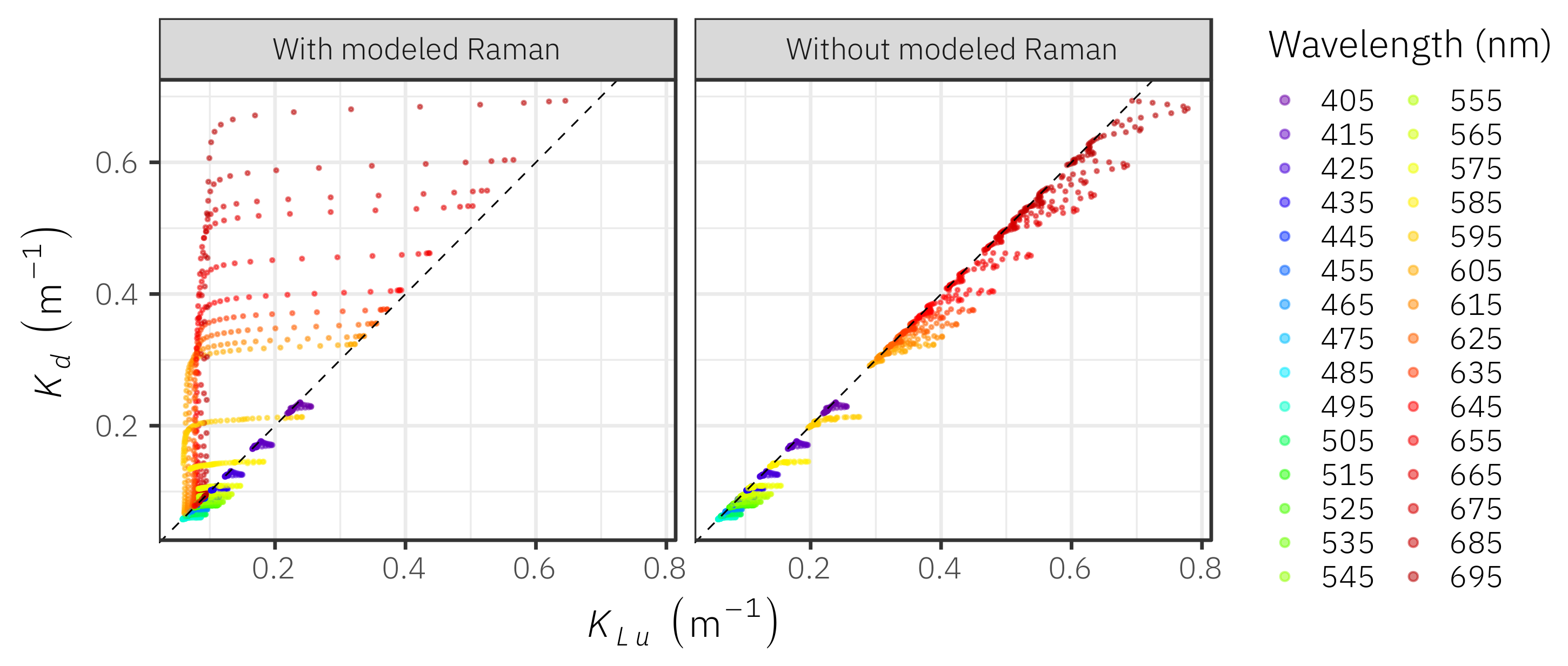
3.3. Inelastic Scattering

Based on in situ data, our results have pointed out that K L u is not a good proxy for K d at longer wavelengths (Figure A3 and Figure A4) because of the effect of Raman scattering. To validate this hypothesis, we used the HydroLight (Sequoia Scientific, Inc., Bellevue, WA, USA) radiative transfer numerical model to calculate theoretical downward irradiance and upward radiance and their associated vertical attenuation coefficients in an open water column in the presence of Raman scattering. The simulation was parametrised using IOPs measured during the field campaign (detailed information can be found in the supplementary section entitled Raman inelastic scattering included in Appendix A). The simulation was able to reproduce the observed decoupling between K d and K L u observed at wavelengths ≥600 nm (Figure A5). These results are generally consistent with previous findings from radiative transfer simulations, which demonstrated the depth and spectral dependencies of diffuse attenuation coefficients as affected by Raman scattering [21,22].

4. Discussion

In the Arctic, melt pond coverage, lead coverage, and ice and snow thickness can vary greatly in both time and space [23,24]. Due to this sea ice heterogeneity, local under-ice measurements of downward irradiance are sometimes characterized by subsurface light maxima (Figure 3). To model such profiles, Laney et al. [9] proposed a semi-empirical parametrisation using two exponential terms (see Equation (3)). Whereas their method might provide adequate estimations of instantaneous downward diffuse attenuation coefficients at specific locations, fitting a double exponential might not be ideal because data are modelled locally and do not provide an adequate description of the average light field ( E d ¯ ( z ) ) as it would be seen, for example, by drifting phytoplankton cells. In such conditions, this paper argues that under-ice irradiance measurements should be analysed in the context of ice and surface properties within a radius of several meters over the horizontal distance because local measurements cannot be used as a proxy of the average light field.
Using in situ light measurements, it was found that E d and L u (and therefore K d and K L u ) were highly correlated below 10 m depth (Figure 4 and Figure 5), even when subsurface light maxima were present (Figure 3). Furthermore, no subsurface light maxima were observed in the in situ upward radiance profiles. The reason is that the L u radiometer measures upwelling photons coming from deeper depth, which have likely undergone more scattering. These photons thus originate from a larger surface area. This reinforces the idea that L u is less influenced by sea ice surface heterogeneity.
Based on Monte Carlo simulations of radiative transfer, our results showed that the average downward irradiance profile, E d ¯ ( z ) , under heterogeneous sea ice cover follows a single-term exponential function, even when melt ponds occupy a large fraction of the study area (Figure 7). This is similar to what is observed under a wavy ice-free surface [10]. However, estimating E d ¯ ( z ) for a given area is not straightforward, as it requires a large number of local profiles under the sea ice. An intuitive alternative to deriving the attenuation coefficient is to use upward radiance, which is less influenced by sea surface heterogeneity compared to downward irradiance (Figure 3, Figure 4 and Figure 5). Monte Carlo simulations showed that a local estimation of K L u was a good proxy for K d ¯ and that using K L u rather than K d provided better estimations of the average downward profile by reducing the average error by approximately a factor of two (Figure 11).
There are at least two main factors influencing the quality of in situ downward irradiance measurements under heterogeneous sea ice. The first factor is the horizontal distance from the centre of the melt pond. Although the relative error of propagating E d ( 0 ) using both K d and K L u showed the same pattern, the largest error occurred when using local estimations of K d directly below the melt pond and up to 10 m from the melt pond edge (Figure 11). In contrast, the relative error associated with the use of K L u was much lower and stabilized just after approximately 10 m from the centre of the melt pond. The second factor driving the relative error of local measurements is the proportion occupied by melt ponds over the area of interest (Figure 11). Indeed, higher proportions of melt pond allow for more light to penetrate in the water column. Hence, local measurements made under surrounding ice are more likely to show subsurface light maxima (see Frey et al. [8]). Accordingly, when melt ponds accounted for 1% of the total area, averaged error in E d ( z ) using K L u was 1.33% but increased to 18% when the melt pond occupied 25% of the total area (Figure 11).

5. Conclusions

Our results show that under spatially heterogeneous sea ice at the surface (and for a homogeneous water column), the average irradiance profile, E d ¯ ( z ) , is well reproduced by a single exponential function. We also showed that propagating E d ( 0 ) using K L u is a better choice compared to K d under heterogeneous sea ice. Nowadays, radiance measurements are becoming more routinely performed during field campaigns, so we argue that one should use K L u when available to propagate E d ( 0 ) through the water column under sea ice. The main difficulty remains in finding good estimates of averaged E d ( 0 ) . In recent years, this has become easier with the development of remotely operated vehicles [3,4,25], remote sensing techniques, and drone imagery. In this study, we used a Monte Carlo approach to model an idealized surface with a single melt pond (Figure 1 and Figure 6). Figure 11 shows that the effect of a melt pond with diameter 5 m is minimized at a horizontal distance of approximately 20 m or more. Therefore, when many melt ponds are characterizing an area, if one has to perform a single profile, measuring an upward radiance profile under bare ice as far away as possible from any melt pond would minimize the error in estimating the area-averaged downward irradiance profile using K L u . Although not representative of a complex Arctic sea ice surface, our simple surface geometry allowed to study the transition from a high to a low transmission sea ice. Further 3D Monte Carlo work could include a more complex geometry of heterogeneous surfaces.

Author Contributions

Conceptualization, P.M., G.B., S.L.-G., E.L. and M.B.; methodology, P.M., G.B., S.L.-G., E.L. and M.B.; field work, G.B., S.L.-G., and M.B.; writing—original draft preparation, P.M.; writing—review and editing, P.M., G.B., S.L.-G., E.L. and M.B.; supervision, M.B.; funding acquisition, M.B.

Funding

The GreenEdge project is funded by the following French and Canadian programs and agencies: ANR (contract #111112), CNES (project #131425), IPEV (project #1164), CSA, Fondation Total, ArcticNet, LEFE and the French Arctic Initiative (GreenEdge project).

Acknowledgments

This project would not have been possible without the support of the Hamlet of Qikiqtarjuaq and the members of the community as well as the Inuksuit School and its principal, Jacqueline Arsenault. The project is conducted under the scientific coordination of the Canada Excellence Research Chair on Remote Sensing of Canada’s New Arctic Frontier and the CNRS and Université Laval Takuvik Joint International laboratory (UMI3376). The field campaign was successful thanks to the contributions of J. Ferland, G. Bécu, C. Marec, J. Lagunas-Morales, F. Bruyant, J. Larivière, E. Rehm, S. Lambert-Girard, C. Aubry, C. Lalande, A. LeBaron, C. Marty, J. Sansoulet, D. Christiansen-Stowe, A. Wells, M. Benoît-Gagné, E. Devred and M.-H. Forget from the Takuvik laboratory, C.J. Mundy and V. Galindo from University of Manitoba, and F. Pinczon du Sel and E. Brossier from Vagabond. We also thank Michel Gosselin, Québec-Océan, the CCGS Amundsen and the Polar Continental Shelf Program for their in-kind contribution in polar logistics and scientific equipment. We thank Laurent Oziel, Jade Larivière and Julien Laliberté for their contribution to radiometry measurements in 2016. This research was enabled in part by support provided by Calcul Québec (www.calculquebec.ca) and Compute Canada (www.computecanada.ca). S.L. Girard was supported by a postdoctoral fellowship from the Natural Sciences and Engineering Research Council of Canada (NSERC). We also acknowledge the Canada First Research Excellence Fund and the Sentinel North Strategy for their financial support. We thank Dariusz Stramski and one anonymous reviewer for their valuable comments which helped to greatly improve the manuscript.

Conflicts of Interest

The authors declare no conflict of interest.

Appendix A

Figure A1. The field campaign was part of the GreenEdge project (www.greenedgeproject.info) which was conducted on landfast ice southeast of the Qikiqtarjuaq Island in the Baffin Bay (67.4797 N, 63.7895 W).
Applsci 08 02693 g0a1

Appendix B. Smoothing Radiance Data

Due to the low scattering coefficients used to reproduce in situ conditions observed during the sampling campaign, radiance profiles were noisy because only few photons were scattered back in the upward direction (note the different y-scales). To overcome this problem, upward radiance data were smoothed using a Gaussian fit accordingly to Equation (A1):
f ( x , φ , μ , σ , k ) = φ e ( x μ ) 2 2 σ 2 + k
where x (m) is the horizontal distance from the center of the melt pond, σ (m) is the standard deviation controlling the width of the curve, φ is the height of the curve peak ( φ = 1 σ 2 π ), μ (m) is the position of the center of the peak, and k an offset coefficient.
Figure A2. Examples showing the number of downward irradiance (A) and upward radiance (B) photons captured by the detectors of the Monte Carlo simulation at different depth ranges (numbers in gray boxes) as a function of the horizontal distance from the melt pond. The red lines represent the fitted Gaussian curves.
Applsci 08 02693 g0a2

Appendix C. Raman Inelastic Scattering

Raman scattering is a process by which photons, interacting with water molecules, lose or gain energy and are scattered at a different wavelength than the one they were originating from. In Figure A3 and Figure A4, one can observe a decoupling between K d and K L u at longer wavelengths, possibly due to inelastic Raman scattering. To validate this hypothesis, we used the HydroLight radiative transfer numerical model to calculate downward irradiance and upward radiance and their associated attenuation coefficients in a water column.
Figure A3. Scatter plots showing the relationships between downward irradiance ( E d ( z ) ) and upward radiance ( L u ( z ) ) between 400 and 700 nm at different depths (numbers in gray boxes). Red lines represent the regression lines of the fitted linear models. Dashed lines are the 1:1 lines. Note the large deviations between the data points and the 1:1 line occurring in the orange and red regions (≥600 nm).
Applsci 08 02693 g0a3
Figure A4. Average determination coefficient R 2 and standard deviation (shaded area) of the regressions between normalized (at 10 m depth) E d ( z ) and L u ( z ) profiles between 400 and 700 nm. At each wavelength, average values were computed from the 83 COPS measurements. A sharp decrease of R 2 occurred at wavelength longer than approximately 575 nm, suggesting a gradual decoupling between E d ( z ) and L u ( z ) profiles at longer wavelengths, possibly due to the effect of inelastic scattering.
Applsci 08 02693 g0a4

HydroLight Simulations

Two HydrolLight simulations were carried out to model downward irradiance and upward radiance with and without taking into account Raman inelastic scattering. The simulations were parameterized using an IOPs profile (ac-s from Sea-Bird Scientific) measured on the first of May 2015 in the Baffin Bay. Simulations were performed with the following characteristics:
  • A surface free of ice.
  • A surface without waves.
  • Sun position at noon for May 1st (solar zenith angle = 45.39 degrees).
  • A cloudless sky.
  • No fluorescence.
  • Using HydroLight default atmospheric parameters.
  • The scattering phase function of water was described by a Fournier-Forand analytic form with a 3% backscatter fraction.
  • EcoLight option was run.
The HydroLight simulations showed a decoupling between K d and K L u starting at around 600 nm when Raman scattering was modelled (Figure A5). Similar decoupling was also observed with the in situ data (see Figure A3).
Figure A5. Scatter plots showing the relationships between K d and K L u calculated from the downward irradiance and upward radiance profiles modelled with and without Raman scattering. The dashed lines represent the 1:1 lines.
Applsci 08 02693 g0a5

References

  1. Kirk, J.T.O. Light and Photosynthesis in Aquatic Ecosystems, 2nd ed.; Cambridge University Press: Cambridge, UK; New York, NY, USA, 1994. [Google Scholar]
  2. Morel, A. An ocean flux study in eutrophic, mesotrophic and oligotrophic situations: The EUMELI program. Deep Sea Res. Part I Oceanogr. Res. Pap. 1996, 43, 1185–1190. [Google Scholar] [CrossRef]
  3. Nicolaus, M.; Katlein, C. Mapping radiation transfer through sea ice using a remotely operated vehicle (ROV). Cryosphere 2013, 7, 763–777. [Google Scholar] [CrossRef] [Green Version]
  4. Katlein, C.; Arndt, S.; Nicolaus, M.; Perovich, D.K.; Jakuba, M.V.; Suman, S.; Elliott, S.; Whitcomb, L.L.; McFarland, C.J.; Gerdes, R.; et al. Influence of ice thickness and surface properties on light transmission through Arctic sea ice. J. Geophys. Res. Ocean. 2015, 120, 5932–5944. [Google Scholar] [CrossRef] [PubMed] [Green Version]
  5. Katlein, C.; Perovich, D.K.; Nicolaus, M. Geometric Effects of an Inhomogeneous Sea Ice Cover on the under Ice Light Field. Front. Earth Sci. 2016, 4. [Google Scholar] [CrossRef]
  6. Lange, B.A.; Flores, H.; Michel, C.; Beckers, J.F.; Bublitz, A.; Casey, J.A.; Castellani, G.; Hatam, I.; Reppchen, A.; Rudolph, S.A.; et al. Pan-Arctic sea ice-algal chl a biomass and suitable habitat are largely underestimated for multiyear ice. Glob. Chang. Biol. 2017, 23, 4581–4597. [Google Scholar] [CrossRef] [PubMed] [Green Version]
  7. Mundy, C.J.; Gosselin, M.; Ehn, J.; Gratton, Y.; Rossnagel, A.; Barber, D.G.; Martin, J.; Tremblay, J.É.; Palmer, M.; Arrigo, K.R.; et al. Contribution of under-ice primary production to an ice-edge upwelling phytoplankton bloom in the Canadian Beaufort Sea. Geophys. Res. Lett. 2009, 36, L17601. [Google Scholar] [CrossRef]
  8. Frey, K.E.; Perovich, D.K.; Light, B. The spatial distribution of solar radiation under a melting Arctic sea ice cover. Geophys. Res. Lett. 2011, 38. [Google Scholar] [CrossRef] [Green Version]
  9. Laney, S.R.; Krishfield, R.A.; Toole, J.M. The euphotic zone under Arctic Ocean sea ice: Vertical extents and seasonal trends. Limnol. Oceanogr. 2017, 62, 1910–1934. [Google Scholar] [CrossRef] [Green Version]
  10. Zaneveld, J.R.V.; Boss, E.; Barnard, A. Influence of surface waves on measured and modeled irradiance profiles. Appl. Opt. 2001, 40, 1442. [Google Scholar] [CrossRef] [PubMed]
  11. Smith, R.C.; Baker, K.S. Analysis of Ocean Optical Data II. In Proceedings of the 1986 Technical Symposium Southeast, Orlando, FL, USA, 7 August 1986; Volume 489, p. 95. [Google Scholar] [CrossRef]
  12. Mobley, C.D. Measuring Radiant Energy, Ocean Optics Web Book. Available online: http://www.oceanopticsbook.info/view/light_and_radiometry/measuring_radiant_energy (accessed on 28 November 2018).
  13. Petrich, C.; Nicolaus, M.; Gradinger, R. Sensitivity of the light field under sea ice to spatially inhomogeneous optical properties and incident light assessed with three-dimensional Monte Carlo radiative transfer simulations. Cold Reg. Sci. Technol. 2012. [Google Scholar] [CrossRef]
  14. Katlein, C.; Nicolaus, M.; Petrich, C. The anisotropic scattering coefficient of sea ice. J. Geophys. Res. Ocean. 2014, 119, 842–855. [Google Scholar] [CrossRef] [Green Version]
  15. Leymarie, E.; Doxaran, D.; Babin, M. Uncertainties associated to measurements of inherent optical properties in natural waters. Appl. Opt. 2010, 49, 5415. [Google Scholar] [CrossRef] [PubMed]
  16. Fournier, G.R.; Forand, J.L. Analytic phase function for ocean water. In Proceedings of the Ocean Optics XII, Bergen, Norway, 26 October 1994; Jaffe, J.S., Ed.; 1994; pp. 194–201. [Google Scholar] [CrossRef]
  17. Mobley, C.D.; Sundman, L.K.; Boss, E. Phase function effects on oceanic light fields. Appl. Opt. 2002, 41, 1035. [Google Scholar] [CrossRef] [PubMed]
  18. Girard, S.L.; Leymarie, E.; Marty, S.; Matthes, L.; Ehn, J.; Babin, M. High angular resolution measurements of the radiance distribution beneath Arctic landfast sea ice during the spring transition. Earth Space Sci. 2018, 5, 30–47. [Google Scholar]
  19. Perovich, D.K. Sea ice and sunlight. In Sea Ice; John Wiley & Sons, Ltd.: Chichester, UK, 2016; Chapter 4; pp. 110–137. [Google Scholar] [CrossRef]
  20. R Core Team. R: A Language and Environment for Statistical Computing; R Foundation for Statistical Computing: Vienna, Austria, 2018. [Google Scholar]
  21. Li, L.; Stramski, D.; Reynolds, R.A. Effects of inelastic radiative processes on the determination of water-leaving spectral radiance from extrapolation of underwater near-surface measurements. Appl. Opt. 2016, 55, 7050. [Google Scholar] [CrossRef]
  22. Berwald, J.; Stramski, D.; Mobley, C.D.; Kiefer, D.A. Effect of Raman scattering on the average cosine and diffuse attenuation coefficient of irradiance in the ocean. Limnol. Oceanogr. 1998, 43, 564–576. [Google Scholar] [CrossRef] [Green Version]
  23. Landy, J.; Ehn, J.; Shields, M.; Barber, D. Surface and melt pond evolution on landfast first-year sea ice in the Canadian Arctic Archipelago. J. Geophys. Res. Ocean. 2014, 119, 3054–3075. [Google Scholar] [CrossRef] [Green Version]
  24. Eicken, H.; Grenfell, T.C.; Perovich, D.K.; Richter-Menge, J.A.; Frey, K. Hydraulic controls of summer Arctic pack ice albedo. J. Geophys. Res. Ocean. 2004, 109, 1–12. [Google Scholar] [CrossRef]
  25. Arndt, S.; Meiners, K.M.; Ricker, R.; Krumpen, T.; Katlein, C.; Nicolaus, M. Influence of snow depth and surface flooding on light transmission through Antarctic pack ice. J. Geophys. Res. Ocean. 2017, 122, 2108–2119. [Google Scholar] [CrossRef] [Green Version]
Figure 1. Spatial configuration used for the 3D Monte Carlo numerical simulations. (A) Surface view showing the percentage of the total area covered by the melt pond over the areas described by the black lines. For each of these areas, light profiles were averaged (see Figure 7). For visualization purpose, lines of the horizontal sampling distances from the centre of the melt pond have been plotted only at 5 m intervals. (B) 2D side view showing the 3D volume for which simulated data were extracted and how photon detectors were placed in the water column. Orange arrows indicate incident light sources.
Applsci 08 02693 g001
Figure 2. Comparison of the under-ice measured downward radiance distribution (the average cosine is ≈0.61, [18]) and the angular distribution of light-emitting source used in the paper.
Applsci 08 02693 g002
Figure 3. Examples of in situ downward irradiance ( E d ( z ) ) and upward radiance ( L u ( z ) ) profiles measured under-ice on 20 June 2016. Note the presence of subsurface maxima in the downward irradiance profiles and the absence of subsurface maxima in the upward radiance profiles.
Applsci 08 02693 g003
Figure 4. Comparison of downward irradiance ( E d ( z ) ) and upward radiance ( L u ( z ) ) for one example light profile measured under-ice. Profiles were normalized to the measured radiometric value at 10 m depth (under the subsurface light maximum) in order to emphasize the similar shape between E d ( z ) and L u ( z ) .
Applsci 08 02693 g004
Figure 5. Scatter plots showing the relationships between the measured K d and K L u in the spectral range between 400 and 580 nm at different depths (numbers in gray boxes). Red lines represent the regression lines of the fitted linear models. Regression equations and determination coefficients ( R 2 ) are also provided in each plot. Dashed lines are the 1:1 lines.
Applsci 08 02693 g005
Figure 6. Cross-sections of simulated downward irradiance and upward radiance fields under a melt pond with a 5 m radius. The logarithm of the normalized number of photons has been used to create the scale for visualization. The normalization has been done using the values modelled at a 0.5 m depth and at a horizontal distance of 50 m from the centre of the melt pond.
Applsci 08 02693 g006
Figure 7. Simulated reference downward irradiance and upward radiance profiles ( E d ¯ ( z ) , L u ¯ ( z ) in relative units) for six different areas with varying proportions of the surface occupied by the melt pond (see Figure 1). Note that none of the averaged irradiance profiles show the same subsurface light maxima as observed with in situ data (see Figure 3).
Applsci 08 02693 g007
Figure 8. Simulated local downward irradiance and upward radiance profiles (expressed in relative units) at different horizontal distances from the centre of the melt pond (see Figure 1) used to compute K d and K L u . These attenuation coefficients were used to propagate surface reference downward irradiance ( E d ( 0 ) , the surface values of the lines in Figure 7) through the water column.
Applsci 08 02693 g008
Figure 9. Diffuse attenuation coefficients calculated from local downward irradiance and upward radiance profiles simulated at different distances from the centre of the melt pond (see Figure 8).
Applsci 08 02693 g009
Figure 10. Reference downward irradiance profiles (thick black lines, in relative units) and propagated irradiance through the water column (coloured lines, in relative units) using local values of K d and K L u (see Figure 8). Light was propagated using the surface reference downward irradiance.
Applsci 08 02693 g010
Figure 11. Relative errors of the predictions calculated as the relative differences between the depth integral of the reference and predicted irradiance profiles.
Applsci 08 02693 g011

