Ocean Color Analytical Model Explicitly Dependent on the Volume Scattering Function

Featured Application

Ocean color remote sensing.

Abstract

An analytical radiative transfer (RT) model for remote sensing reflectance that includes the bidirectional reflectance distribution function (BRDF) is described. The model, called ZTT (Zaneveld-Twardowski-Tonizzo), is based on the restatement of the RT equation by Zaneveld (1995) in terms of light field shape factors. Besides remote sensing geometry considerations (solar zenith angle, viewing angle, and relative azimuth), the inputs are Inherent Optical Properties (IOPs) absorption a and backscattering b_b coefficients, the shape of the particulate volume scattering function (VSF) in the backward direction, and the particulate backscattering ratio. Model performance (absolute error) is equivalent to full RT simulations for available high quality validation data sets, indicating almost all residual errors are inherent to the data sets themselves, i.e., from the measurements of IOPs and radiometry used as model input and in match up assessments, respectively. Best performance was observed when a constant backward phase function shape based on the findings of Sullivan and Twardowski (2009) was assumed in the model. Critically, using a constant phase function in the backward direction eliminates a key unknown, providing a path toward inversion to solve for a and b_b. Performance degraded when using other phase function shapes. With available data sets, the model shows stronger performance than current state-of-the-art look-up table (LUT) based BRDF models used to normalize reflectance data, formulated on simpler first order RT approximations between r_rs and b_b/a or b_b/(a + b_b) (Morel et al., 2002; Lee et al., 2011). Stronger performance of ZTT relative to LUT-based models is attributed to using a more representative phase function shape, as well as the additional degrees of freedom achieved with several physically meaningful terms in the model. Since the model is fully described with analytical expressions, errors for terms can be individually assessed, and refinements can be readily made without carrying out the gamut of full RT computations required for LUT-based models. The ZTT model is invertible to solve for a and b_b from remote sensing reflectance, and inversion approaches are being pursued in ongoing work. The focus here is with development and testing of the in-water forward model, but current ocean color remote sensing approaches to cope with an air-sea interface and atmospheric effects would appear to be transferable. In summary, this new analytical model shows good potential for future ocean color inversion with low bias, well-constrained uncertainties (including the VSF), and explicit terms that can be readily tuned. Emphasis is put on application to the future NASA Plankton, Aerosol, Cloud, and ocean Ecosystem (PACE) mission.

1. Introduction

Radiative transfer (RT) approximations linking inherent optical properties (IOPs), such as spectral absorption a(λ) (m⁻¹) and spectral backscattering b_b(λ) (m⁻¹) to ocean color remote sensing reflectance R_rs(λ) are vital to interpreting R_rs because it is not possible to analytically invert the full RT equation [1,2]. Once forward RT approximations are developed, inversions can then be explored to solve for IOPs from R_rs and subsequently ocean biogeochemical properties [3]. Ocean color R_rs(λ) (sr⁻¹) here is defined as L_w(λ)/E_d(λ), or water leaving radiance (W m⁻² sr⁻¹ nm⁻¹) normalized to above water downwelling irradiance (W m⁻² nm⁻¹) (see Reference [4] for complete definitions of all optical parameters and Appendix A,

Table A1. Notation.

Symbol	Description	Units
a	total absorption coefficient	m−1
ax	absorption coefficient, where subscript x = w, p, d, ph, g, pg, pico, and micro specifies water, particulate, non-phytoplankton particulate, phytoplankton, dissolved, particulate plus dissolved, picoplankton, and microplankton	m−1
a*	specific absorption coefficient	m2 mg−1
b	total scattering coefficient	m−1
bp	particulate scattering coefficient	m−1
bf	forward scattering coefficient	m−1
bbx	backscattering coefficient, where subscript x = w and p specifies water and particulate	m−1
${\tilde{b}}_b$	backscattering ratio	-
${\tilde{b}}_{bp}$	particulate backscattering ratio	-
β	total volume scattering function (VSF)	m−1 sr−1
βx	volume scattering function (VSF), where subscript x = w and p specifies seawater and particulate	m−1 sr−1
c	total attenuation coefficient	m−1
[Chl]	chlorophyll concentration	mg m−3
δx	error, where subscript x = abs and rel specifies absolute and relative	-
Ex	planar irradiance, where subscript x = d, ds, and dd specifies downwelling, diffuse downwelling, and direct downwelling	W m−2 nm−1
Eod	downwelling scalar irradiance	W m−2 nm−1
f	model coefficient for relating irradiance reflectance to bb/a	-
fb, fL	radiance shape factors	-
Φ	azimuth angle relative to solar plane	°, rad
G	model coefficient for above-surface remote sensing reflectance	sr−1
ψ	scattering angle	°, rad
H	fraction of diffuse downwelling light (Eds/Ed)	-
ηbb	fraction of total backscattering contributed by bbw	-
Kx	diffuse attenuation coefficient, where subscript x = Lu, u, d, and ∞ specifies upwelling radiance, upwelling irradiance, downwelling irradiance, and asymptotic	m−1
Lu	upwelling radiance	W m−2 nm−1 sr−1
Lw	water-leaving radiance	W m−2 nm−1 sr−1
λ	Wavelength	nm
$M_d^{+}$	Atmospheric component of ${\overline{\mu }}_d$	-
$M_d^{*}$	IOP component of ${\overline{\mu }}_d$	-
${\overline{\mu }}_{\infty }$	average cosine of the asymptotic light field	-
${\overline{\mu }}_d$	average cosine of the downwelling light field	-
μw	cosine of the in-water solar zenith	-
np	particulate refractive index, relative to water	-
P	phase function (β/b)	sr−1
Px	particulate phase function (βp/bp), where subscript x = p, ps, and pl specifies particulate, particulate small-dominant, and particulate large-dominant	sr−1
Pbb,x	backward particulate phase function (βp/bbp), where subscript x = ST and FF specifies functions from References [26,44]	sr−1
Q	ratio of upwelling irradiance to nadir radiance	sr
rrs	remote sensing reflectance, the ratio of upwelling subsurface radiance to downwelling irradiance	sr−1
Rrs	remote sensing reflectance, the ratio of water-leaving radiance to downwelling irradiance	sr−1
Rd	scaling factor for ad	-
Rg	scaling factor for ag	-
Sf	mixing factor for aph	-
θx	zenith angle, where x = s and v specifies solar and viewing	°, rad
θs’	above water solar zenith angle	°, rad
v	exponent of empirical spectral bp function	-
V	atmospheric horizontal visibility	km
ω	albedo (b/c)	-
${\Psi }_{K_{Lu}}$	ratio of diffuse upwelling attenuation coefficient to asymptotic attenuation coefficient	-
z	depth	m

for notation).

Ocean color expressions to date have almost exclusively relied on first order approximations of RT relating R_rs to b_b/a through a proportionality represented as f/Q [5,6,7,8], or to b_b/(a + b_b) with multi-term polynomial expressions based originally on Gordon et al. [9] with coefficients represented as l or G ([9,10,11,12]; see review by Werdell et al. [13]). The coefficients describing the relationship between R_rs and IOPs are detailed in look-up tables (LUTs), or a neural network in the case of [8], with dependencies on geometry (i.e., solar zenith, viewing angle, relative azimuth) and in some cases wavelength, wind speed, atmospheric conditions, and/or chlorophyll concentration [Chl]. The LUTs are generated from full RT computations with so-called synthetic data sets where IOPs and their interrelationships are assumed and referenced to [Chl]. LUT coefficients are thus also implicitly dependent on IOPs.

These ocean color relationships have been tremendously useful to the ocean color community for decades. Morel [14] discusses the first order analytical relationship and the empiricism necessary to invert. Coefficients describing the relationship between R_rs and IOPs are dependent on the bidirectional reflectance distribution function (BRDF), which describes the transformation of downwelling irradiance for different solar zenith angles into the distribution of upwelling radiance. Morel et al. [7] describe the current state-of-the-art BRDF model (herein referred to as M02), currently implemented operationally by the ocean color community (NASA Ocean Biology Processing Group (OBPG); [15]) to convert L_w measured at any viewing geometry to a conceptual “exact normalized” L_w, ${\left[L_w\right]}_N^{ex}$, with Sun at zenith and nadir viewing in a non-attenuating atmosphere. This allows any measurement at any Sun-viewing geometry to be directly intercompared. Inversion algorithms to derive IOPs are then typically applied to ${\left[L_w\right]}_N^{ex}$ and are often based on the same type of first order R_rs to IOP approximation [13,16]. The current semi-analytical algorithm (SAA) application to water-leaving radiances is thus a two-step process (after applying calibration coefficients, georeferencing, and atmospheric correction): (1) A BRDF correction to carry out the conversion to ${\left[L_w\right]}_N^{ex}$, followed by (2) application of an inversion algorithm to derive IOPs (see [13]).

A key potential source of uncertainty in current SAA approaches is associated with the volume scattering function (VSF; β(ψ) m⁻¹ sr⁻¹, where ψ is scattering angle), and this uncertainty is ambiguously dispersed in both steps. The VSF dependency is of paramount importance; as Morel and Gentili [5] note, the BRDF “… is essentially controlled by the shape of the VSF ….” Historically, very few measurements of the VSF have been available to develop and test SAAs. The M02 BRDF tables were developed from extensive RT modeling using VSF shapes (also known as phase functions P(ψ), defined as the VSF normalized to total scattering, P(ψ) = β(ψ)/b, with units sr⁻¹) tied to estimated chlorophyll concentrations [Chl]. To obtain P(ψ) for modeling, Morel et al. [7] first mixed two phase functions for populations dominated by large and small particles representing high and low [Chl] extremes, respectively, and then mixed that particulate phase function with the phase function for molecular seawater to a degree that was also linked to estimated [Chl]. The [Chl] estimate was initially derived from R_rs with an empirical band ratio algorithm. Uncertainty is thus associated with how close the assumed P(ψ) used in the BRDF modeling matches the actual P(ψ) associated with any given L_w measurement. While the M02 model has been validated in Case 1 waters with atmospheric conditions and IOPs that presumably agree with the underlying atmospheric and bio-optical models [17,18], there have been limited attempts to assess any embedded phase function uncertainties with actual VSF measurements in diverse water types [19,20]. No subsequent BRDF approach has demonstrated enhanced performance for Case 1 waters relative to the M02 approach while being feasible to implement for ocean color. However, Talone et al. [21] have recently shown the Lee et al. [11] LUT-based approach was more accurate for Case 2 waters sampled in the Adriatic, Baltic, and Black Seas.

Uncertainty also arises from exclusively using the b_b term in the inversion algorithm, i.e., in step two of the SAA approach described above. Effort has been devoted to trying to correct this uncertainty by layering additional VSF dependence in the f/Q proportionality [22]. Interestingly, after the current M02 BRDF normalization is applied (i.e., measurement geometry transferred to Sun at zenith and nadir viewing), the scattering parameter that should be most closely linked to ${\left[L_w\right]}_N^{ex}$, and thus presumably should provide the lowest associated uncertainties in IOP retrievals, is β(π) if single scattering is assumed, which is typically a good approximation [23]. We are not aware however of any algorithm using β(π) in lieu of b_b. The practical but still arbitrary choice of converting measured L_w to ${\left[L_w\right]}_N^{ex}$ with Sun at zenith and nadir viewing may thus not optimize uncertainties in inversion algorithms. The parameter β(π) is almost completely unknown in the ocean, as there are virtually no direct measurements of β(π) in the literature and typical models of particle scattering with simplified particle shapes do not account for possible particle-particle coherent scattering that may cause significant, but poorly understood, enhancement near β(π) [24]. For example, a recent estimate of b_b/β(π) made with a combination of airborne lidar and in situ b_b measurements [25] was 50% the value expected from extrapolation of available β measurements [26].

Although the M02 BRDF correction as currently applied can be considered “conceptual” at L_w(0,π) without creating a problem from a geometry point of view (i.e., L_w at any viewing geometry can be corrected to a conceptual standard L_w at another geometry as long as it is consistent), it will be problematic if we try to develop algorithms based on β(π) to reduce uncertainties because the necessary data for algorithm development and validation are lacking. This would also suggest a possible benefit in using the BRDF correction to obtain ${\left[L_w\right]}_N^{ex}$ at another unique geometry (solar zenith, viewing angle, and azimuth), one that was representative of single scattering at an angle that we can measure directly with available instrumentation. To minimize the magnitude of BRDF correction, this angle could be chosen as the centroid angle of the maximum in the frequency distribution of in-water single scattering angles observed for polar orbiting satellites, which is about 150° (Figure 1). Since we can accurately measure β at or near 150° with commercially available instrumentation (e.g., WET Labs ECO, In-situ Marine Optics IMO-SC6, and legacy HOBI Labs Hydroscat sensors), there would appear to be potential to reduce uncertainties with β(150°)-based algorithms matched to a β(150°)-based BRDF correction using M02 relative to the current b_b-based algorithms applied to a β(π)-based BRDF correction. In the former approach, uncertainties associated with the phase function are thus mostly restricted to the BRDF correction step.

Herein we explore a different approach, working with a RT expression from Zaneveld [27,28] that explicitly incorporates a dependency on VSF shape, as well as specific viewing geometry. A path to inversion to IOPs is also presented where SAA steps 1 and 2 mentioned above are combined in a single relationship and uncertainties related to VSF shape and other parameters can be directly assessed. This approach has several potential benefits, including (1) a single, fully analytical and invertible expression describing the RT process for all remote sensing geometries, (2) optimal retention of native RT relationships with more degrees of freedom than the first order approximation, directly linked to physically meaningful terms, (3) all parameters including the VSF are explicit in the model with readily characterized uncertainties, (4) model can be readily enhanced by tuning one or more terms rather than developing new LUTs from complete recomputations of full RT, and (5) native viewing geometries produce scattering at angles that can be resolved with available instrumentation. A challenge in an explicitly VSF-dependent approach is amenability to inversion, as some information about the phase function is ostensibly required [1,20]. However, it should be pointed out this is also the case with any model, including the M02 BRDF correction, and subsequent inversion algorithms and their inherent assumptions about VSF shape. In fact, as is assessed herein, the same assumptions of M02 in linking changes in VSF shape with an independent estimate of chlorophyll can be directly applied to this RT model, with the benefit of being able to directly quantify associated errors.

In this paper we focus on the performance of a forward implementation of the Zaneveld expression using a modified formulation in terms of IOPs that is now amenable to inversion. Performance of the inversion to IOPs is being fully assessed in ongoing work. A key advance promoting inversion is the finding by Sullivan and Twardowski [26] that the shape of the particulate VSF in the backward direction is relatively constant for a wide range of water types, and so may be represented by a constant function in an algorithm without introducing significant error. Importantly, we have also now overcome a limitation in practically assessing this approach by collecting a database of measured VSFs resolved over a large dynamic range concurrently with other high quality IOPs and radiometry under ideal cloud-free environmental conditions [29].

2. Forward Model Development

Zaneveld [27,28] derived an exact restatement of the RT equation assuming a plane-parallel, optically deep water column in terms of upwelling radiance L_u in viewing direction θ_v:

$$\frac{L_u\left({\theta }_s,{\theta }_v,\varphi \right)}{E_{od}}=\frac{f_b\left({\theta }_s,{\theta }_v,\varphi \right)\frac{b_b}{2\pi }}{-\cos \left({\theta }_v\right)K_{L_u}\left({\theta }_s,{\theta }_v,\varphi \right)+c-f_L\left({\theta }_s,{\theta }_v,\varphi \right)b_f},$$

(1)

where E_od is the scalar downwelling irradiance, K_Lu is the attenuation coefficient for upwelling radiance, b_f is forward scattering, and c is the attenuation coefficient. Parameters f_b and f_L are light field shape factors representing the path radiance term of the RT equation [27,28]. Factor f_b describes the redirection of downwelling radiance into the upwelling viewing angle for a given VSF and is normalized to the redirection that would be observed if the VSF was isotropic. Factor f_b is thus directly linked to the shape of the VSF in the backward direction. The factor f_L is defined similarly but describes the redirection of upwelling radiance into the upwelling viewing angle and is thus directly linked to the shape of the near forward VSF. These shape factors are expected to vary within a relatively narrow range near unity. All terms are a function of depth z and wavelength λ. The Zaneveld expression does not account for any inelastic processes, such as molecular Raman scattering or fluorescence [30,31,32,33]. Using physically reasoned approximations for f_b including the assumption of single scattering, the following was obtained by Zaneveld ([28]; his Equation (14)):

$$\frac{L_u\left({\theta }_s,{\theta }_v,\varphi \right)}{E_{od}}=\frac{\beta \left(\psi \right)}{-\cos \left({\theta }_v\right)K_{Lu}\left({\theta }_s,{\theta }_v,\varphi \right)+c-f_L\left({\theta }_s,{\theta }_v,\varphi \right)b_f},$$

(2)

where β is the VSF (including water) and ψ is the in-water scattering angle formed between peak incident sunlight at solar zenith angle θ_s and scattered light traveling in viewing direction (θ_v,Φ), where cos(ψ) = cos(θ_s)cos(θ_v) − sin(θ_s)sin(θ_v)cos(φ). Azimuth φ is relative to the Sun’s direction. Zenith angles θ are in-water, refracted through the air-sea interface and determined from a vertically downward direction. For nadir viewing, ψ = π − θ_s and −cos(θ_v) = 1 in the denominator. Note approximations of Equation (2) provided in Zaneveld [28] assumed only nadir viewing while we retain the full BRDF functionality here.

In theoretical analyses, Weidemann et al. [34] showed b_b retrievals based on the Zaneveld expression had errors as large as −20% and +40%. However, an extraordinarily wide range of VSF shapes was applied in their simulated data, including VSF shapes for specific particulate subcomponents, such as bacteria, minerals, and phytoplankton. These populations were considered separately as quasi-monodispersions with phase function shapes computed from Lorenz-Mie theory, i.e., assuming homogeneous spheres. These phase function shapes thus had large oscillations with respect to angle, structure that we now know is extremely unrealistic for VSFs representative of bulk in situ particle populations (e.g., [26,35,36,37]). Weidemann et al. also showed with these phase functions that the Zaneveld approximation of the shape factor at nadir viewing, i.e., f_b ≈ 2πβ(π − θ_s)/b_b, had an average error of only 5% (their Figure 11) and this included overcast conditions that would not occur in remote sensing. To our knowledge, the only study attempting to test the Zaneveld model with directly measured data was He et al. [20] with a subset of the NOMAD data set, which included no VSF measurements, where performance for the BRDF component of the model was comparable to the current state-of-the-art [7,11].

Equation (2) demonstrates the direct link between $L_u\left({\theta }_s,{\theta }_v,\varphi \right)$ and β(ψ). However, for the Zaneveld expression to be a practical tool for ocean color, the terms $K_{Lu}$ and f_L must be expressed in terms of IOPs. Furthermore, the IOPs in the model should ideally be coefficients that are closely linked to reflectance and directly measurable with good accuracy using existing sensor technology. For example, the term in the denominator [$c-f_L\left({\theta }_s,{\theta }_v,\varphi \right)b_f$] has two IOPs that are difficult to determine directly because of acceptance angle issues with standard transmissometer designs [38,39]. However, since f_L is close to unity, this term is also closely related to a + b_b, immediately recognizable from commonly used first order approximations. Goals of the next several sections are: 1) To represent Equation (2) entirely in terms of such IOPs, 2) to rework in terms of the commonly used remote sensing reflectance L_u/E_d, since these are the measurements currently available in validation data sets, and 3) to include the inelastic effects associated with water Raman scattering.

2.1. Diffuse Attenuation of Upwelling Radiance $K_{Lu}$

For the term $K_{Lu}$, Zaneveld [28] suggested an assumption of equivalency to $K_{\infty }$, the diffuse attenuation coefficient in the asymptotic regime. Asymptotic theory is based on the principle that the shape of the light field with depth gradually transforms from being dependent on the incident surface light field to being constant, azimuthally symmetric (so L is only a function of θ), and dependent only on IOPs. Attenuation coefficients for all aspects of the light field, i.e., for all radiances and therefore all irradiances, are equivalent in the asymptotic regime and are also IOPs. This is a critical assumption for the purposes of model development since K can then be described only in terms of IOPs. Zaneveld justified the assumption, even though the omnidirectional light field in surface waters is far from asymptotic, due to the decoupling of upwelling radiances to downwelling radiance distributions. Measurements of upwelling radiance fields from the 1960s and 1970s showed a near constant shape and attenuation rate with depth. Recently, Twardowski and Tonizzo [40] confirmed this assumption in RT simulations with no more than 3% error when the sun was at solar zenith and the following relationship held for above water solar zeniths θ_s′ up to 75°:

$$\frac{K_{Lu}-K_{\infty }}{K_{\infty }}=F\left({\theta }_s\prime \right)=f_1{\theta }_s{\prime }^4+f_2{\theta }_s{\prime }^3+f_3{\theta }_s{\prime }^2+f_4{\theta }_s\prime +f_5,$$

(3)

which included a full range of possible natural water types. Coefficients f are provided in Appendix A,

Table A2. Equation Coefficients. Full 15 decimal scaled fixed point precision in MATLAB is provided to ensure accuracy in calculations.

Equation	Symbol	Value
Equation (3)	$f_1$	−5.98948784303628 × 10−8
	$f_2$	5.95904039870752 × 10−6
	$f_3$	−6.975283717755 × 10−4
	$f_4$	2.07111856771792 × 10−3
	$f_5$	2.69046922858858 × 10−2
Equation (4)	$f_{A1}$	−3.79435531537314 × 10−7
	$f_{A2}$	2.42117623125973 × 10−4
	$f_{A3}$	−5.76056692150838 × 10−2
	$f_{A4}$	6.04944577004764
	$f_{A5}$	−236.166389774491
Equation (16)	$e_1$	−3.37021020153209 × 10−12
	$e_2$	2.25040435584125 × 10−10
	$e_3$	−2.25897880448836 × 10−9
	$e_4$	4.98402568695743 × 10−10
	$e_5$	−3.67440351688922 × 10−8
	$e_6$	4.02677827509591 × 10−7
	$e_7$	−2.52448256032736 × 10−8
	$e_8$	2.09631870150827 × 10−6
	$e_9$	−2.43068373614361 × 10−5
	$e_{10}$	5.98295717192273 × 10−7
	$e_{11}$	−5.36922068813161 × 10−5
	$e_{12}$	6.84105803724285 × 10−4
	$e_{13}$	−5.34168078899319 × 10−6
	$e_{14}$	4.95201118318049 × 10−4
	$e_{15}$	−6.09578731164684 × 10−3
	$e_{16}$	5.32097604773773 × 10−4
	$e_{17}$	−2.91276619216202 × 10−2
	$e_{18}$	0.589340234481004
Equation (17)	$m_{d,1}^{*}$	0.00611094400155735
	$m_{d,2}^{*}$	−0.00104841847722295
	$m_{d,3}^{*}$	0.0498255758922950
	$m_{d,4}^{*}$	−0.0117672820980625
	$m_{d,5}^{*}$	0.128019358635212
	$m_{d,6}^{*}$	−0.0429896134897322
	$m_{d,7}^{*}$	0.103528931695373
	$m_{d,8}^{*}$	0.950921179229178

. Angle θ_s′ is related to θ_s by Snell’s Law, i.e., θ_s′ = sin⁻¹(1.34 sin(θ_s)). Only nadir viewing was considered in the simulations for $K_{Lu}$ in Equation (3), and we make the assumption that $K_{Lu}$ for other viewing angles that define a specific scattering angle ψ can be approximated by Equation (3) with nadir viewing geometry after assigning a θ_s′ that provides an equivalent in-water ψ. For example, for θ_s′ = 60°, θ_s will be 40.3° and ψ will be 139.7° for nadir viewing; we assume the resulting F(60°) will also be applicable to any off-nadir viewing angle with ψ = 139.7°. This assumption has been verified using Hydrolight RT simulations (methodology addressed in Section 3.2) to no worse than 2% in the solar plane and no worse than 5% within the upwelling hemisphere for in-water scattering angles consistent with remote sensing (i.e., Figure 1). This assumption implies a rotational reference frame, where the first order determinant of radiance field shape in the model, i.e., ψ, is preserved. Two potential drawbacks of this assumption are (1) the influence of skylight may be skewed in the rotated reference frame, and (2) the range of viewing angles is restricted since the smallest ψ is ~134° for underwater nadir viewing. The range ψ > 134°, however, comprises >95% of the expected scattering angles that will be measured by the PACE imager (Figure 1). Further work with field measurements is needed to verify this assumption. Reformulating Equation (3) in terms of dependency on the in-water scattering angle, we obtain:

$$F\left(\psi \right)=f_{A1}{\psi }_{}^4+f_{A2}{\psi }_{}^3+f_{A3}{\psi }_{}^2+f_{A4}{\psi }_{}+f_{A5}.$$

(4)

Coefficients f_A are provided in Appendix A, Table A2.

From Gershun’s Law we can set $K_{\infty }=a/{\overline{\mu }}_{\infty }$, where ${\overline{\mu }}_{\infty }$ is the average cosine of the asymptotic light field. After inserting Equation (4) into Equation (2) and allowing for c = a + b, the following is obtained:

$$\frac{L_u\left({\theta }_s,{\theta }_v,\varphi \right)}{E_{od}}\cong \frac{\beta \left(\psi \right)}{a\left(1-\cos \left({\theta }_v\right){\Psi }_{K_{Lu}}\left(\psi \right) {\overline{\mu }}_{\infty }{}^{-1}\right)+b-f_L\left({\theta }_s,{\theta }_v,\varphi \right)b_f},$$

(5)

$$\mathrm{where}{\Psi }_{K_{Lu}}\left(\psi \right)=K_{Lu}/K_{\infty }=\left[1+F\left(\psi \right)\right].$$

(6)

The parameter Ψ_KLu is assumed spectrally independent with errors over the full range of possible water types estimated at <2% [40]. Dividing numerator and denominator of Equation (5) by b_b, we obtain:

$$\frac{L_u\left({\theta }_s,{\theta }_v,\varphi \right)}{E_{od}}\cong \frac{\beta \left(\psi \right)}{b_b}/{\left[\frac{a}{b_b}\left(1-\cos \left({\theta }_v\right){\Psi }_{K_{Lu}}\left(\psi \right){\overline{\mu }}_{\infty }{}^{-1}\right)+f_L\left({\theta }_s,{\theta }_v,\varphi \right)\left(1-{\tilde{b}}_b{}^{-1}\right)+{\tilde{b}}_b{}^{-1}\right]}^{},$$

(7)

where ${\tilde{b}}_b$ = b_b/b is the backscattering ratio. For IOPs we now have the backward phase function in the numerator; in the denominator we have the recognizable b_b/a, as well as ${\tilde{b}}_b$, an IOP that incorporates information on bulk particle composition (see Section 2.4; [41]), and is not typically associated with ocean color remote sensing vis-à-vis the common first order approximation of r_rs assumed proportional to b_b/a.

2.2. Average Cosine of the Asymptotic Light Field ${\overline{\mu }}_{\infty }$

The ${\overline{\mu }}_{\infty }$ term in Equation (7) must be expressed in terms of IOPs to invert. Using a fit to theoretical calculations of radiance fields by Prieur and Morel [42], Zaneveld [28] recommended 1/${\overline{\mu }}_{\infty }$ be modeled empirically with respect to the single scattering albedo ω (=b/c) using a quadratic fit. Additionally, through more detailed RT computations, Berwald et al. [43] found a 4th order dependency of ${\overline{\mu }}_{\infty }$ on the albedo.

In the study by Twardowski and Tonizzo [40], ${\overline{\mu }}_{\infty }$ was parameterized in terms of b_b/a instead of ω, including an assessment across a full range of environmentally representative phase function shapes using the Fournier-Forand analytical model [44,45]. The data set used in the assessment was not a representative synthetic data set (i.e., [46]), as it included a full range of possible b_b/a values, possible phase functions, and permutations thereof. Representing ${\overline{\mu }}_{\infty }$ in terms of b_b/a has two distinct advantages. First, b_b and a can be measured with commercially available in situ instrumentation with accuracies of a few percent [47,48,49] to enable performance assessment for algorithms. Parameters c and b cannot be measured without significantly larger errors, typically >25–50%, because of the acceptance of near forward scattered light in conventional transmissometer designs [38,39]. Secondly, b and c are not parameters that are closely linked to r_rs without additional information, whereas b_b and a are (e.g., Gordon et al. [50]), and a goal here is to represent the entire model in terms of b_b and a to enable inversion.

The Twardowski and Tonizzo [40] parameterization also explicitly depended on η_bb, the fraction of b_b attributable to molecular scattering, η_bb = b_bw/(b_bp + b_bw) [6]. The natural range for η_bb is from ~0 to ~0.98 [40,51], and the range used for b_b/a was 10⁻⁴ to 10⁻¹. Since the water components of η_bb may be assumed known [52], the effective unknown here is b_bp. After extending the analysis from Reference [40] to include near zero b_b/a and increased resolution in η_bb, the resulting fit was obtained for ${\overline{\mu }}_{\infty }$:

$$\begin{array}{ll}{\overline{\mu }}_{\infty }\left(\frac{b_b}{a},{\eta }_{bb}\right)\approx & \left[m_1{\left(\log {\eta }_{bb}\right)}^3+m_2{\left(\log {\eta }_{bb}\right)}^2+m_3\log {\eta }_{bb}+m_4\right]{\left(\log \frac{b_b}{a}\right)}^3\\ & +\left[m_5{\left(\log {\eta }_{bb}\right)}^3+m_6{\left(\log {\eta }_{bb}\right)}^2+m_7\log {\eta }_{bb}+m_8\right]{\left(\log \frac{b_b}{a}\right)}^2\\ & +\left[m_9{\left(\log {\eta }_{bb}\right)}^3+m_{10}{\left(\log {\eta }_{bb}\right)}^2+m_{11}\log {\eta }_{bb}+m_{12}\right]\log \frac{b_b}{a}\\ & +m_{13}{\left(\log {\eta }_{bb}\right)}^3+m_{14}{\left(\log {\eta }_{bb}\right)}^2+m_{15}\log {\eta }_{bb}+m_{16}.\end{array}$$

(8)

Coefficients m are provided in Appendix A, Table A2. Fits to simulated data were again made with the polyfit function from MATLAB. Absolute errors %δ_abs for this fit vary from 0.19 to 3.5 for η_bb ranging from 0.98 to 0.0098, respectively. Since both b_b/a and η_bb are spectrally dependent, ${\overline{\mu }}_{\infty }$ will be as well (not shown for clarity).

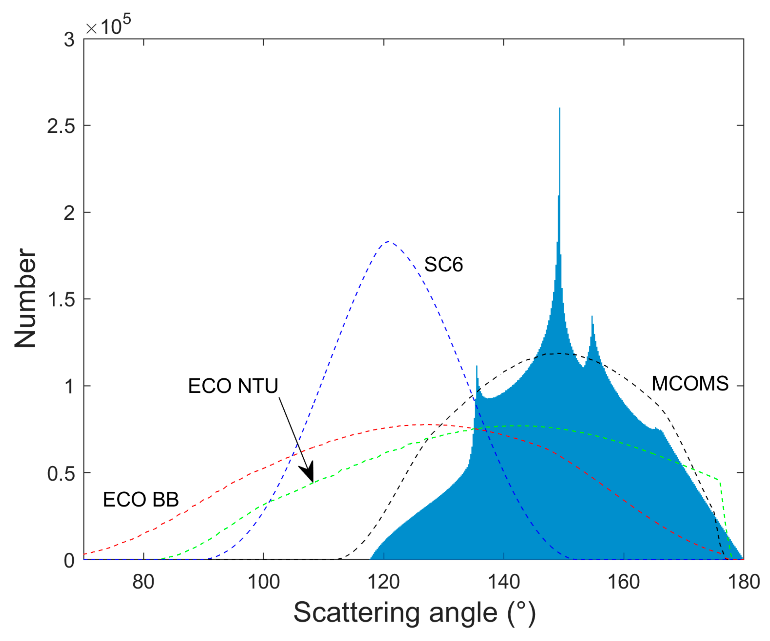
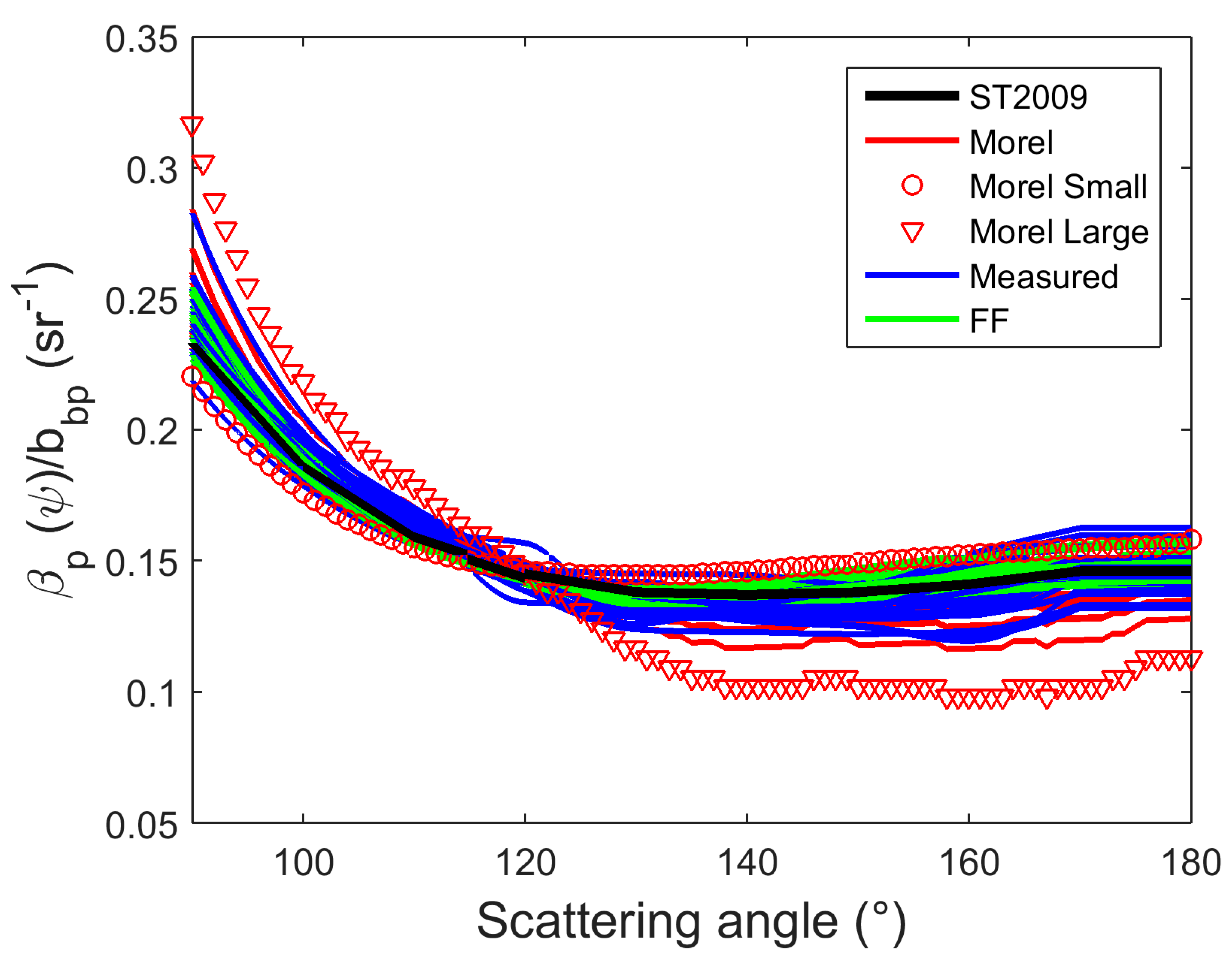
2.3. Backward Phase Function β(ψ)/b_b

The scattering parameters in Equation (7) must be expanded into water and particulate components. Expanding β(ψ)/b_b gives:

$$\frac{\beta \left(\psi \right)}{b_b}=\frac{{\beta }_p\left(\psi \right)+{\beta }_w\left(\psi \right)}{b_{bp}+b_{bw}},$$

(9)

where the p and w subscripts represent particles and molecular seawater, respectively. In Equation (9), the pure seawater terms, which are temperature and salinity specific, can be directly computed with an estimated error of no more than 2% [52]. Introducing a term for the particulate phase function in the backward direction, P_bb(ψ) = β_p(ψ)/b_bp, Equation (9) then becomes:

$$\frac{\beta \left(\psi \right)}{b_b}=\frac{P_{bb}\left(\psi \right)b_{bp}+{\beta }_w\left(\psi \right)}{b_{bp}+b_{bw}}.$$

(10)

Note b_bp and b_bw both have spectral dependencies as does β/b_b, and the unknowns are b_bp(λ) and P_bb(ψ). Equation (10) can be easily rewritten in terms of η_bb, with the same unknowns. In coastal waters where η_bb is near zero, β_p >> β_w, b_bp >> b_bw, and β(ψ)/b_b will be approximated by P_bb(ψ). For clear ocean waters, phase functions are represented by a mixture of both particles and pure seawater with VSF shapes dependent on η_bb.

2.4. Backscattering Ratio ${\tilde{b}}_b$

Expanding the backscattering ratio ${\tilde{b}}_b$ = b_b/b in Equation (7) we obtain:

$$\frac{b_b}{b}=\frac{b_{bp}+b_{bw}}{b_p+b_w}=\frac{b_{bp}+b_{bw}}{b_{bp}/{\tilde{b}}_{bp}+b_w},$$

(11)

where ${\tilde{b}}_{bp}$ is the particulate backscattering ratio. This ${\tilde{b}}_{bp}$ is the “true” ${\tilde{b}}_{bp}$, distinct from the ${\tilde{b}}_{bp}$ typically derived from measurements that include c data from transmissometers with significant acceptance angle errors (e.g., [38,39]) (we note models linking particle biogeochemical properties and measured ${\tilde{b}}_{bp}$ should account for the acceptance angle of c measurements [41,53]). Bootstrapping exercises using Equation (7) readily show an impact on reflectance of up to several percent when ${\tilde{b}}_{bp}$ is varied over the full ~0.003 to ~0.03 dynamic range observed in the oceanic environment [41,53,54,55,56]. All terms have spectral dependencies.

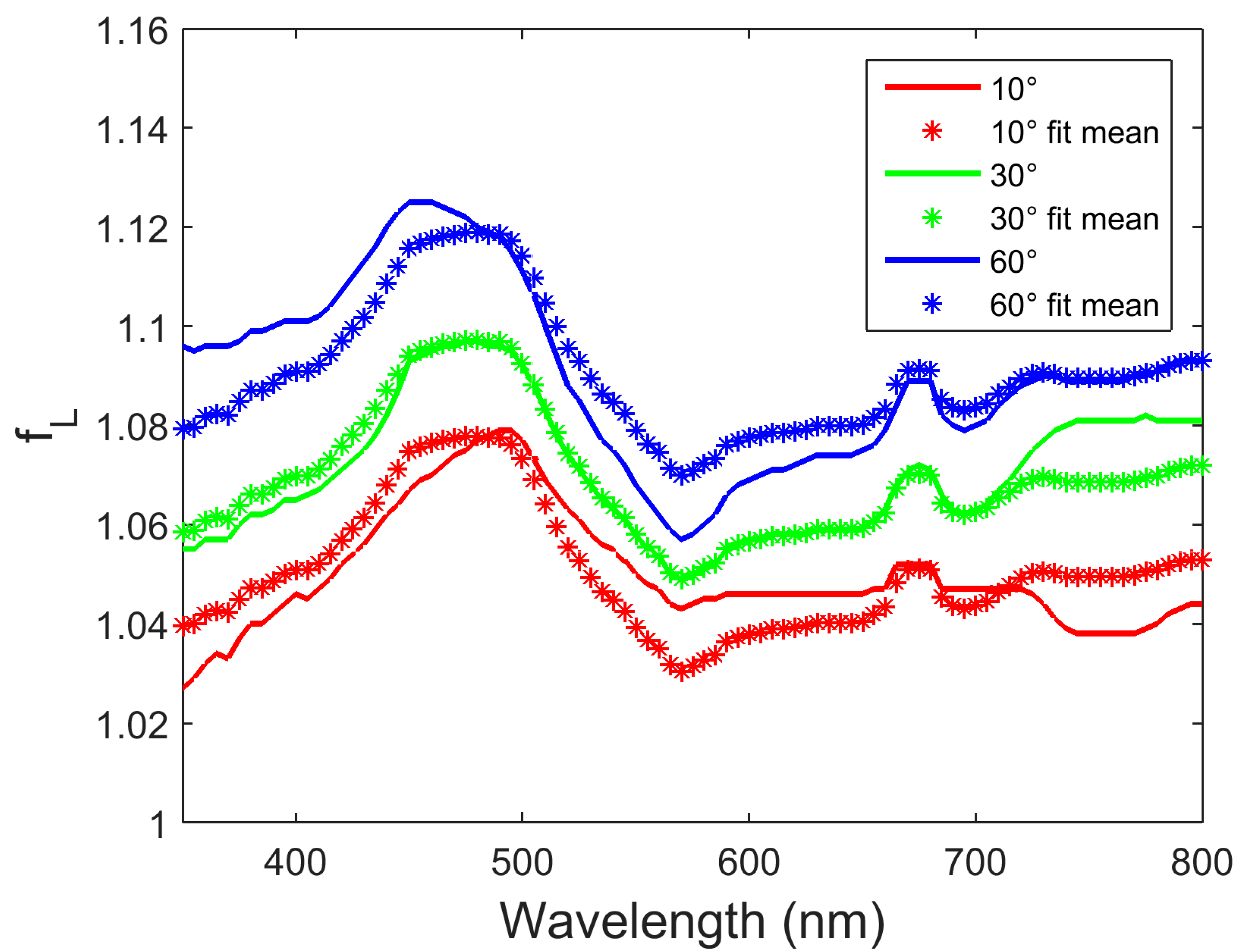
2.5. Shape Factor f_L

Zaneveld [28] recommended the term f_L, i.e., the dimensionless upwelling radiance shape factor, could be set to 1.05 with small error. The natural range was estimated at 1 to 1.12 [27]. In the Results, we develop a new model for this term.

2.6. Remote Sensing Reflectance Formulation

Nearly all ocean RT algorithm work over the last several decades has used reflectance defined as L_u/E_d instead of L_u/E_od. Zaneveld [28], however, pointed out, as is evident from Equation (1), L_u/E_od is most closely aligned with RT theory. The irradiance parameter E_od is also less dependent on solar zenith angle than E_d. Furthermore, sensor technology has been available to measure E_od, historically from companies Biospherical (www.biospherical.com), Satlantic (www.satlantic.com), and Trios (www.trio.de). Nonetheless, since nearly all field data over the last several decades has focused on E_d, any testing and validation of the RT model described here requires modification in terms of E_d. Substituting $E_d/E_{od}={\overline{\mu }}_d$ (the average cosine of downwelling radiance, just below the air-water interface) into Equation (7) gives:

$$r_{rs}\cong \frac{1}{{\overline{\mu }}_d}\frac{\beta \left(\psi \right)}{b_b}/{\left[\frac{a}{b_b}\left(1-\cos \left({\theta }_v\right){\Psi }_{K_{Lu}}{\overline{\mu }}_{\infty }{}^{-1}\right)+f_L\left(1-{\tilde{b}}_b{}^{-1}\right)+{\tilde{b}}_b{}^{-1}\right]}^{},$$

(12)

where r_rs is the classically known remote sensing reflectance just below the water surface. Full dependencies of variables not shown for clarity.

2.7. Average Cosine of the Downwelling Light Field ${\overline{\mu }}_d$

A model for ${\overline{\mu }}_d$ is now required in the expression from Equation (12). If the sky is ignored and we assume a negligible fraction of the incident solar beam is scattered in the near-surface, a reasonable first-order approximation of ${\overline{\mu }}_d$ should be μ_w ≡ cos(θ_s). Adding in a cardioidal radiance distribution for skylight, Morel and Prieur [57] obtained:

$$\frac{1}{{\overline{\mu }}_d}\approx \frac{0.6}{{\mu }_w}+\frac{0.4}{0.859},$$

(13)

and noted that for sun angles between 8° and 62°, ${\overline{\mu }}_d$ varied only from 0.79 to 0.94. Thus, even without knowledge of solar zenith angle, a median value could be used with an accuracy better than 10%.

Numerator values of 0.6 and 0.4 in Equation (13) represent the fractions of direct (E_dd/E_d) and diffuse (H = E_ds/E_d) downwelling light, respectively, which together equal unity. These values primarily depend on θ_s’ and horizontal visibility V, the latter of which depends on aerosol optical thickness (AOT). For 20° ≤ θ_s’ ≤ 60° and for H between 0.2 and 0.5, the variability of ${\overline{\mu }}_d$ is ~7% for a fixed θ_s’.

The term ${\overline{\mu }}_d$ can be factorized in two parts, one part dependent on the IOPs, the other dependent on the atmospheric conditions and geometry:

$${\overline{\mu }}_d\left({\theta }_s^{\prime },V,\frac{b_b}{a},{\eta }_{bb}\right)\approx M_d^{+}\left({\theta }_s\prime ,V\right)\times M_d^{*}\left(\frac{b_b}{a},{\eta }_{bb}\right).$$

(14)

The atmospheric component can be represented as:

$$M_d^{+}\left({\theta }_s\prime ,V\right)=\raisebox{1ex}{${\left[\frac{1-H\left({\theta }_s\prime ,V\right)}{{\mu }_w}+\frac{H\left({\theta }_s\prime ,V\right)}{0.859}\right]}^{-1}$}\!\left/ \!\raisebox{-1ex}{$P^3\left[\cos \left({\theta }_s\prime \right)\right]$}\right..$$

(15)

As mentioned, Morel and Prieur [57] assumed H = 0.4. Gregg and Carder [58] later provided a relationship for H as a function of θ_s′ and V that included skylight. Specifically, the results of ([58]; their Figure 4) can be fit as follows:

$$\begin{array}{ll}H\left({\theta }_s^{\prime },V\right)=& \left[e_1{V}^2+e_{2}V+e_3\right]{\theta }_s{\prime }^5+\left[e_4{V}^2+e_{5}V+e_6\right]{\theta }_s{\prime }^4\\ & +\left[e_7{V}^2+e_{8}V+e_9\right]{\theta }_s{\prime }^3+\left[e_{10}{V}^2+e_{11}V+e_{12}\right]{\theta }_s{\prime }^2\\ & +\left[e_{13}{V}^2+e_{14}V+e_{15}\right]{\theta }_s^{\prime }+e_{16}{V}^2+e_{17}V+e_{18}.\end{array}$$

(16)

Coefficients e are provided in Appendix A, Table A2. Note the typical default value used in Hydrolight is V = 15 km.

The P³ term in the $M_d^{+}$ relationship is a 3rd order polynomial in cos$\left({\theta }_s\prime \right)$ to correct where Morel and Prieur’s original approximation deviates from the Gregg and Carder relationship at large ${\theta }_s\prime$. The P³ term is:

$$P^3\left[\cos \left({\theta }_s\prime \right)\right]=0.7792{\cos }^3\left({\theta }_s\prime \right)-1.7366{\cos }^2\left({\theta }_s\prime \right)+1.1551\cos \left({\theta }_s\prime \right)+0.7842.$$

The IOP-dependent component $M_d^{*}$ was modeled using the approach in [40] with the extended b_b/a range and η_bb resolution discussed in Section 2.2. The final fitted relationship is:

$$\begin{array}{ll}{M}_d^{*}\left(\frac{b_b}{a},{\eta }_{bb}\right)=& \left[m_{d,1}^{*}\log {\eta }_{bb}+m_{d,2}^{*}\right]{\left(\log \frac{b_b}{a}\right)}^3+\left[m_{d,3}^{*}\log {\eta }_{bb}+m_{d,4}^{*}\right]{\left(\log \frac{b_b}{a}\right)}^2\\ & +\left[m_{d,5}^{*}\log {\eta }_{bb}+m_{d,6}^{*}\right]\log \frac{b_b}{a}+m_{d,7}^{*}\log {\eta }_{bb}+m_{d,8}^{*}.\end{array}$$

(17)

Coefficients $m_d^{*}$ are provided in Appendix A, Table A2. Absolute percent error with this relationship relative to computations using full radiative transfer (Hydrolight, see Section 3.2) varies from 0.06% to 0.4% across all θ_s’. Error for the full ${\overline{\mu }}_d$ expression is <1%. Spectral dependency enters the expression through the V term, which is dependent on spectral AOT.

2.8. Including Inelastic Water Raman Effects

The molecular water Raman scattering contribution to r_rs can be included in Equation (12) as an additive term, resulting in the expression:

$$\begin{array}{c}{r}_{rs}\left({\theta }_s,{\theta }_v,\varphi ,V,a,b_b\right)\cong r_{rs,Raman}\left({\theta }_s\prime ,a,b_b\right)+\frac{1}{{\overline{\mu }}_d\left({\theta }_s^{\prime },V,\frac{b_b}{a},{\eta }_{bb}\right)}\frac{\beta \left(\psi \right)}{b_b}/\\ {\left[\frac{a}{b_b}\left(1-\cos \left({\theta }_v\right){\Psi }_{K_{Lu}}\left(\psi \right){\overline{\mu }}_{\infty }{\left(\frac{b_b}{a},{\eta }_{bb}\right)}^{-1}\right)+f_L\left({\theta }_s,{\theta }_v,\varphi \right)\left(1-{\tilde{b}}_b{}^{-1}\right)+{\tilde{b}}_b{}^{-1}\right]}^{}.\end{array}$$

(18)

Full dependencies for all parameters in the model are shown except for λ; all parameters exhibit dependence on λ in the model except for ${\Psi }_{K_{Lu}}\left(\psi \right)$. We note a similar approach has been taken in adding water Raman effects in other reflectance models (e.g., [59]; reviewed in [13]). The term r_rs,Raman can be derived according to Westberry et al. ([60]; see their Equation (7)) with inputs of above water (z = 0⁺) downwelling irradiance E_d(0⁺,θ_s’), a, and b_b. The NASA Generalized IOP (GIOP) inversion model implementation [16] also currently uses this Raman formulation. Terms for other inelastic effects, such as fluorescence from dissolved organic matter and pigments may also be added if representative models are available.

2.9. ZTT Model Summary

Equation (18) is the final model for ocean color reflectance defined as L_u/E_d, called the ZTT model hereafter. In Equation (18) the ${\overline{\mu }}_d$ term is approximated by Equation (14), the β(ψ)/b_b term approximated by Equation (10), the ${\Psi }_{K_{Lu}}$ term described by Equations (4) and (6), the ${\overline{\mu }}_{\infty }$ term described by Equation (8), and ${\tilde{b}}_b$ represented by Equation (11). The ultimate assignment of the f_L term is addressed in the Results. The geometry variables, E_d(0⁺,θ_s’), V, and molecular water scattering parameters in the above can be considered knowns. The model is fully spectral. Key unknowns are b_b and a (or b_b/a and η_bb), and since pure seawater absorption a_w in the visible is considered known with good accuracy [61] the effective unknowns are b_bp and absorption by non-water constituents a_pg. The two additional unknowns are P_bb(ψ) and ${\tilde{b}}_{bp}$. In the forward implementation here, these four parameters must be provided from direct measurements or through some assumptions. In the inversion implementation, these are the parameters that may be solved through techniques to minimize errors in the expression if there are enough spectral bands (i.e., degrees of freedom) in r_rs, although a priori assumptions may be required for P_bb(ψ) and ${\tilde{b}}_{bp}$.

For ocean color reflectance defined as L_u/E_od, the simpler relationship in Equation (7) can be used. Water Raman effects can still be considered by applying an algorithm, such as in Reference [60].

3. Methods

3.1. Synthetic Dataset

A synthetic data set referenced to [Chl] was developed to test the ZTT model and develop an expression for the f_L term (see Section 4.1). Twenty values of [Chl] were assumed, logarithmically spaced between 0.01 and 30 mg m⁻³. Total absorption coefficient (a) was represented by a sum of four components:

$$a\left(\lambda \right)=a_w\left(\lambda \right)+a_{ph}\left(\lambda \right)+a_d\left(\lambda \right)+a_g\left(\lambda \right).$$

(19)

Pure water absorption a_w was taken from Reference [61]. Phytoplankton absorption a_ph was calculated from chlorophyll concentration [Chl] and from spectrally averaged absorption coefficients of micro- and pico-plankton (${\overline{a}}_{micro}\left(\lambda \right)$ and ${\overline{a}}_{pico}\left(\lambda \right)$, respectively) [62]:

$$a_{ph}\left(\lambda \right)=\left[Chl\right]*\left(\left[S_f{\overline{a}}_{pico}\left(\lambda \right)\right]+\left[\left(1-S_f\right){\overline{a}}_{micro}\left(\lambda \right)\right]\right),$$

(20)

where S_f = [0.25, 0.5, 0.75] is the shape mixing factor. Non-algal particulate absorption a_d was given by [63]:

$$a_d\left(\lambda \right)=a_d\left(440\right)*e^{-0.011\left(\lambda -440\right)},$$

(21)

where a_d(440) is equal to R_d a_ph(440), with R_d = [0.05, 0.1, 0.5, 1, 2]. Similarly, we used an exponentially decaying expression for the absorption of chromophoric dissolved organic matter, a_g [64]:

$$a_g\left(\lambda \right)=a_g\left(440\right)*e^{-0.014\left(\lambda -440\right)},$$

(22)

where a_g(440) is equal to R_g a_ph(440), with R_g = [0.1, 0.3, 0.5, 1, 2].

Total backscattering b_b was represented by the sum of water and particulate components:

$$b_b\left(\lambda \right)=b_{bp}\left(\lambda \right)+b_{bw}\left(\lambda \right).$$

(23)

To derive particulate backscattering b_bp, total particulate scattering b_p was first empirically estimated at 550 nm [65]:

$$b_p\left(550\right)=0.416{\left[Chl\right]}^{0.766},$$

(24)

and then extrapolated spectrally [66]:

$$b_p\left(\lambda \right)=b_p\left(550\right)*{\left(\frac{\lambda }{550}\right)}^{v\left(\left[Chl\right]\right)},$$

(25)

where v([Chl]) = 0.5(log[Chl] − 0.3) when 0.01 ≤ [Chl] ≤ 2 mg m⁻³ and v([Chl]) = 0 when [Chl] > 2 mg m⁻³. The empirical relationship from [41] between the particulate backscattering ratio ${\tilde{b}}_{bp}$ and [Chl] was then used to derive b_bp:

$$b_{bp}=b_p{\tilde{b}}_{bp}=b_p*0.0096{\left[Chl\right]}^{-0.253}.$$

(26)

Pure seawater backscattering b_bw was calculated according to Zhang et al. [52].

3.2. Radiative Transfer Simulations

RT simulations of r_rs were performed with Hydrolight (Sequoia Scientific, Bellevue, WA), following the procedure in Tonizzo et al. [29]. Fournier-Forand analytical phase functions were derived for each [Chl] iteration following the method of Mobley et al. [67].

Inelastic water Raman scattering was not included in the simulations for the synthetic data set, as this is separately addressed in the model (Equation (18)); fluorescence from any seawater constituents was also not considered. Note water Raman effects were included in full RT simulations for all field data (see [29]). Output wavelengths ranged from 350 to 800 nm at 5 nm resolution. Hydrolight default atmospheric parameters were used for all runs. Computations were run for θ_s′ of 10, 30 and 60°. Altogether, 1500 different IOP permutations based on [Chl] were simulated for each θ_s’.

3.3. Field Data Sets

Model performance was assessed using two aggregate data sets. The first is a high quality data set of 23 stations from the Ligurian Sea, waters around the Marine Optics BuoY (MOBY) west of Lanai, the southern California coast, and the New York Bight, collected in 2008 and 2009 as part of NASA Spectral Ocean Radiance Transfer Investigation and Experiment (SORTIE) and NASA Ocean Color Validation (OCVAL) exercises. Radiometric closure was assessed in detail for these data by Tonizzo et al. [29]. [Chl] ranged from 0.24 to 23.85 mg m⁻³. The VSF was directly measured using the custom Multi-Angle SCattering Optical Tool (MASCOT) [26,36] and radiometric uncertainties were rigorously assessed by Voss et al. [68]. Here we use WET Labs ac-9 absorption measurements corrected for scattering using independent VSF measurements (i.e., the VSF98P correction [29]; also see Stockley et al. [49] for detailed evaluation of this correction). The second data set is the NASA NOMAD database, where 80 data records were identified containing the parameters needed for performance assessments here, i.e., a, b_b, ${\tilde{b}}_{bp}$, [Chl], and r_rs. [Chl] ranged from 0.23 to 10.68 mg m⁻³ in this data set.

3.4. Depth Weighting IOPs

Depth-weighted contributions of IOPs to water-leaving radiance were derived after Zaneveld et al. [69] using a 2-stream, first derivative approximation. The approach finds the IOP for a conceptual homogeneous ocean that reproduces the water-leaving radiance observed in a specific stratified ocean case. The remote sensing depth weighting for generic IOP X is:

$$\langle X\rangle ={{\displaystyle \int }}_{z=0}^{z=\infty }Xf\left(z\right)dz,\mathrm{where}f\left(z\right)=\frac{d}{dz}exp\left[-2{{\displaystyle \int }}_{z=0}^{z=\infty }K\left(z\right)dz\right].$$

(27)

The exponential term can also be found in Gordon and Clark [70], where it is mentioned the 2K(z) term should actually be K_u + K_d, but approximating with K_d alone was not expected to lead to appreciable errors. Several approximations of K_d in terms of IOPs are available from the literature (e.g., [71,72]). The approximation by Lee et al. [73] for averaged K_d within the euphotic zone is used here and conveniently represented in terms of a, b_b and above water solar zenith θ_s′:

$${\overline{K}}_d=\left(1+0.005{\theta }_s\prime \right)a+4.18\left(1-0.52e^{-10.8a}\right)b_b.$$

(28)

For evaluating RT approximations, all IOP terms should ideally be weighted together. For example, Zaneveld et al. [69] considered the simple R ∝ b_b/a approximation and demonstrated that <b_b>/<a> was not equivalent to <b_b/a> for an IOP stratified ocean. However, b_b and a are considered independently in the model here and an ultimate objective is to invert the approximation to derive b_b and a independently, so each IOP was individually depth weighted. For all stations sampled in the validation data set, the difference between surface b_b and depth weighted b_b was <1%; with a, this was also the case for most stations, but reached a difference of 5% for one station sampled.

3.5. Metrics for Error Assessment

Mean absolute percent error (MAPE), $\%{\delta }_{abs}$, is a commonly used metric in assessing performance in r_rs match ups:

$$\%{\delta }_{abs}=100*\frac{{\delta }_{abs}}{\overline{y}}, {\delta }_{abs}=\frac{{{\displaystyle \sum }}_{i=1}^n\left|y_i-\widehat{y_i}\right|}{n}.$$

(29)

The MAPE metric takes into account the absolute magnitude of the residuals, giving them equal weight. Other commonly used metrics include root mean square error (RMSE), a measure of accuracy and potential forecasting errors in simulating r_rs when the errors may be assumed to be unbiased and normally distributed [74]. RMSE gives greater weight to larger errors than δ_abs. Since bias errors are often expected to be more significant than random, normally distributed errors in simulations, %δ_abs is expected to be the most appropriate metric to assess match ups [29]. Other common metrics (e.g., [75]) are shown in the following plots as appropriate. Also see Werdell et al. [13] for a detailed discussion of performance metrics.

4. Results

4.1. Developing an Expression for the f_L Term

Dynamics of f_L were explored in the synthetic data set. As found by Hoge et al. [76], dependencies on wavelength and θ_s′ were most important, and an average spectral shape f_L,ave(λ) scaled to solar zenith according to sin(θ_s’) was ultimately found to be most representative (Figure 2):

$$f_L\left({\theta }_s^{\prime },\lambda \right)=f_{L,ave}\left(\lambda \right)\left[0.05959\sin \left({\theta }_s\prime \right)+0.9728\right].$$

(30)

Function f_L,ave(λ) is provided in Appendix A,

Table A3. $f_{L,ave}\left(\lambda \right)$ function, see Equations (30) and (31).

Wavelength	Value	Wavelength	Value	Wavelength	Value
350	0.990	505	1.018	655	0.992
355	0.990	510	1.013	660	0.993
360	0.992	515	1.009	665	0.998
365	0.992	520	1.005	670	1.000
370	0.992	525	1.002	675	1.001
375	0.995	530	0.999	680	1.000
380	0.997	535	0.996	685	0.995
385	0.997	540	0.995	690	0.994
390	0.998	545	0.992	695	0.993
395	1.000	550	0.989	700	0.994
400	1.000	555	0.987	705	0.994
405	1.000	560	0.985	710	0.996
410	1.002	565	0.982	715	0.997
415	1.003	570	0.981	720	0.999
420	1.006	575	0.982	725	1.000
425	1.008	580	0.983	730	1.000
430	1.010	585	0.984	735	1.000
435	1.013	590	0.986	740	0.999
440	1.016	595	0.987	745	0.999
445	1.020	600	0.988	750	0.999
450	1.023	605	0.988	755	0.999
455	1.024	610	0.989	760	0.999
460	1.025	615	0.989	765	0.999
465	1.025	620	0.989	770	0.999
470	1.026	625	0.990	775	1.000
475	1.026	630	0.990	780	1.000
480	1.026	635	0.990	785	1.001
485	1.026	640	0.990	790	1.002
490	1.026	645	0.990	795	1.002
495	1.024	650	0.990	800	1.002
500	1.022

. Equation (30) was developed by minimizing residual errors between results from full radiative transfer and the ZTT model for each wavelength and each solar zenith angle for the full synthetic data set. Spectral shapes for f_L were relatively consistent in the results, so the term f_L,ave(λ) was derived from an average for these results after spectral normalization. The scaling factor in brackets was a suitable function to minimize errors with respect to solar zenith angle. Only nadir viewing was again considered in the simulations for f_L, and we again make the assumption from Section 2.1 that f_L for other viewing angles that define a specific in-water scattering angle ψ can be approximated by f_L observed at the nadir viewing geometry with equivalent ψ. The potential caveats mentioned in Section 2.1 apply here as well. Restating Equation (30) in terms of ψ, the following is obtained:

$$f_L\left(\psi ,\lambda \right)=f_{L,ave}\left(\lambda \right)\left[0.07762\sin \left(\psi \right)+1.0405\right].$$

(31)

Similarities between f_L,ave(λ) and a typical ocean absorption spectrum are noted (Figure 2), resulting from the effects of multiple scattering, where higher relative scattering (lower relative absorption) promotes a radiance field closer to that which would result from isotropic scattering, i.e., where f_L approaches unity.

Figure 3A shows results deriving r_rs using the ZTT model for the synthetic data set, applying the approximation from Equation (31) for f_L and using all synthetic data IOPs as input. This match up is, thus, effectively assessing combined errors in the ZTT model from the approximations of f_L, f_b, $K_{Lu}$, and ${\overline{\mu }}_d$. We note f_L was specifically optimized to this data set, so in this respect Figure 3A shows what may be considered a best-case matchup. MAPE %δ_abs for the full data set was relatively small at 2.68%. The largest errors were observed in three r_rs spectra, with the model showing overestimation bias centered around 570 nm. These spectra were associated with the highest [Chl] modeled in the data set and lowest ${\tilde{b}}_{bp}$.

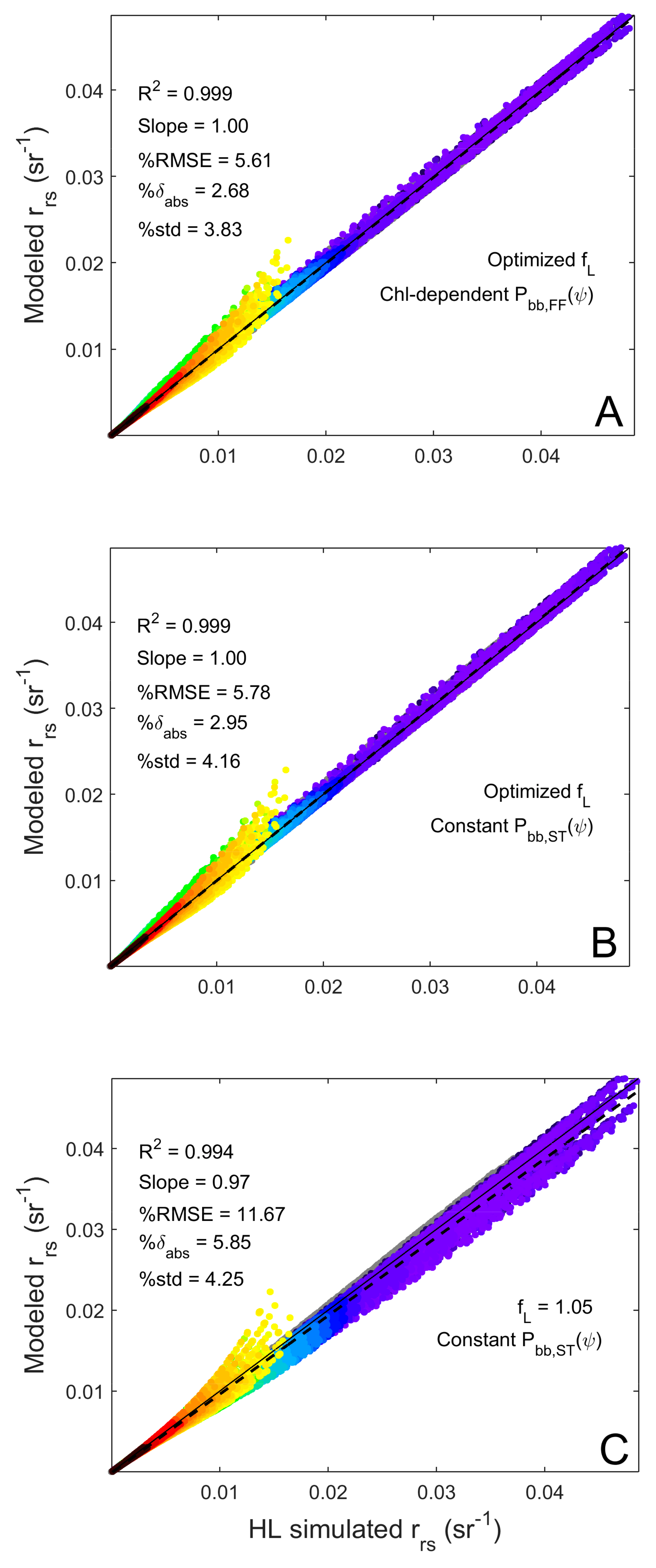
4.2. Assessing Assumption of Constant β_p(ψ)/b_bp

Sullivan and Twardowski [26] found a high degree of consistency in the shape of the particulate VSF in the backward direction, i.e., β_p(ψ)/b_bp, for a large data set covering a wide dynamic range in bulk particle composition. Deviations from this relationship were no more than 5% through the entire backward angular range. While it is well known the phase function shape over the full angular range varies substantially (e.g., [37,41,45,77]), only the shape in the backward direction that is important for remote sensing and the ZTT model is considered here.

If we assume β_p(ψ)/b_bp is a constant shape P_bb,ST(ψ) after Sullivan and Twardowski [26] in the ZTT model, replacing P_bb,FF(ψ,${\tilde{b}}_{bp}$) from the synthetic data set, errors increase by only ~0.3% (Figure 3B). We assume P_bb,ST(ψ) is constant spectrally after [41] and others. This result is significant, as it demonstrates the potential for eliminating one of the key unknowns in the ZTT model. We note that an averaged Fournier-Forand phase function in the backward direction could be used in the model, which would enhance the analytical character of the model, but the Sullivan and Twardowski [26] averaged phase function, derived from extensive measurements in a wide range of water types, may be more representative of the natural environment. This is assessed further in the next section. Figure 3C shows results of setting f_L to a constant 1.05 after [28] and using a constant P_bb,ST(ψ). MAPE increases significantly to 5.85%, showing the importance of using the f_L model in the ZTT. Each of the three distinct data groupings along the 1:1 relationship are associated with the individual solar zeniths that were used, i.e., 10, 30, and 60°, highlighting the influence of the f_L model in removing the effects of solar zenith. All ZTT model runs hereafter use the f_L model from Equation (31). The constant backward phase function P_bb,ST(ψ) is used unless another phase function is specified.

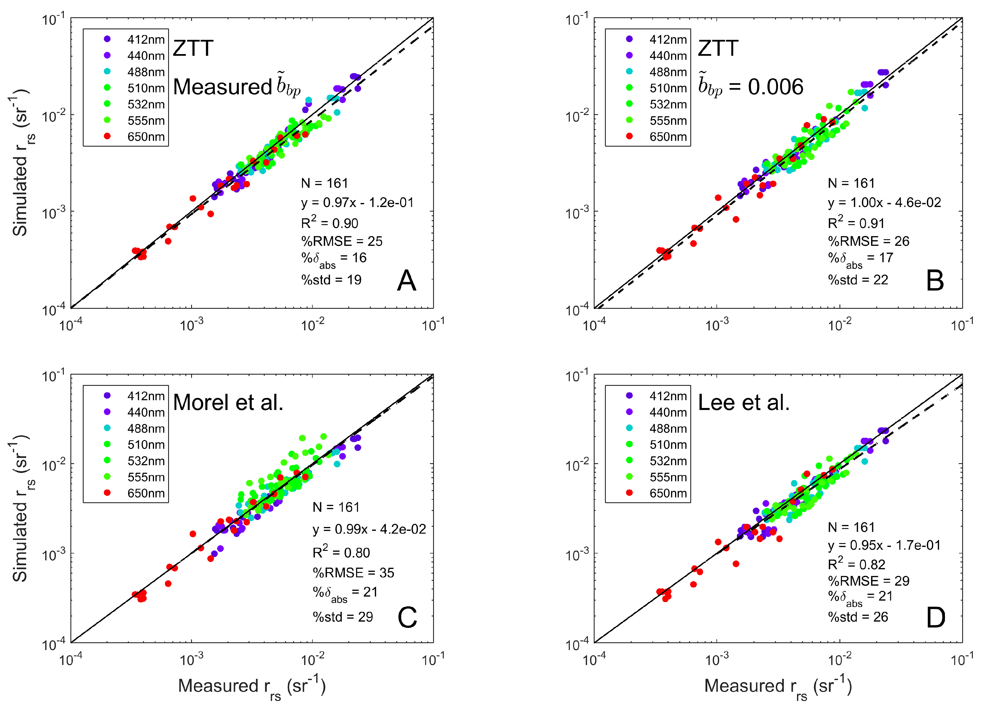
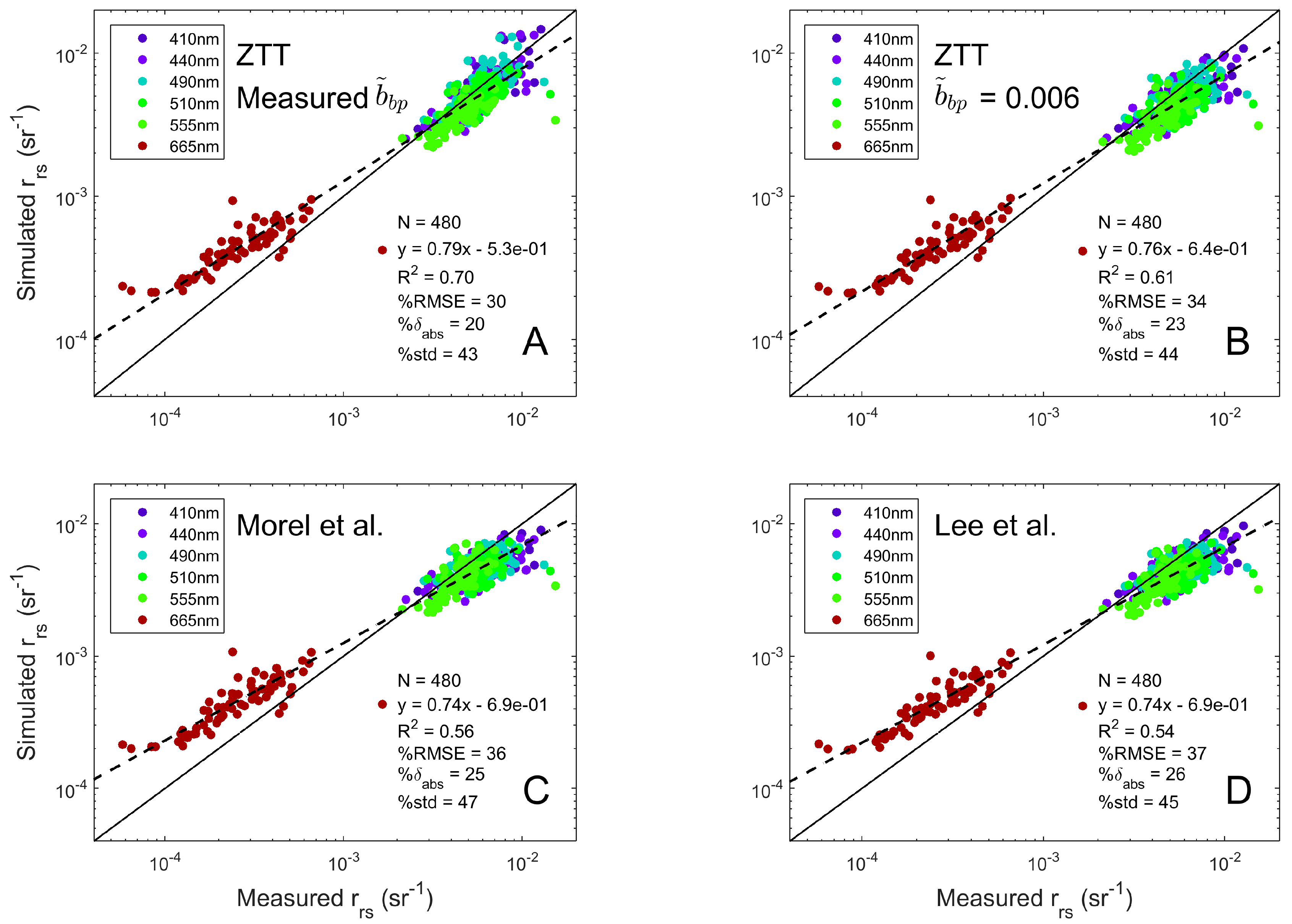
4.3. Assessment with High Quality Validation Data

Figure 4A shows results for the ZTT model, with inputs of constant P_bb,ST(ψ) and direct measurements of a_pg, b_bp, and ${\tilde{b}}_{bp}$, compared to measured r_rs for the validation data set [29]. MAPE %δ_abs was 16% for all λ (summarized in

Table 1. Summary MAPE %δ_abs results for simulated or calculated r_rs vs measured r_rs for all λ.

Approach	βp(ψ)/bbp Input	${\tilde{\mathit{b}}}_{\mathit{b}\mathit{p}}$ Input	%δabs
			SORTIE and OCVAL (23 Stations) 1	NOMAD (80 Stations)
Full RT 2	directly measured	N/A	17	nd 4
Full RT 2	Fournier-Forand 3	measured	20	nd 4
ZTT	directly measured	measured	17	nd 4
ZTT	Fournier-Forand 3	measured	19	25
ZTT	Pbb,ST(ψ)	measured	16	20
ZTT	Pbb,ST(ψ)	0.005	18	22
ZTT	Pbb,ST(ψ)	0.006	17	23
ZTT	Pbb,ST(ψ)	0.008	18	25
ZTT	Pbb,ST(ψ)	0.010	19	27
ZTT	Pbb,ST(ψ)	0.015	22	29
ZTT	Large and small population phase functions with ${\tilde{b}}_{bp}$ of 0.19% and 1.4%, blended according to [Chl] 5	measured	23	26
Morel et al. [7] (M02)	Large and small population phase functions with ${\tilde{b}}_{bp}$ of 0.19% and 1.4%, blended according to [Chl] 5	N/A	21	25
Lee et al. [11] (L11)	Blend of Petzold6 average and 1% ${\tilde{b}}_{bp}$ Fournier-Forand 3	N/A	21	26

¹ see [29]; ² Hydrolight; ³ derived from ${\tilde{b}}_{bp}$ according to [67]; ⁴ not determined; ⁵ algorithm of [7]; ⁶ [79].

; spectral %δ_abs provided in

Table 2. Summary MAPE %δ_abs results for calculated r_rs vs measured r_rs for each λ, for SORTIE and OCVAL data sets (see Figure 4) and NOMAD data (see Figure 6).

Approach	βp (ψ)/bbp Input	${\tilde{\mathit{b}}}_{\mathit{b}\mathit{p}}$ Input	λ (nm)	%δabs
				SORTIE and OCVAL (23 Stations)	NOMAD (80 Stations)
ZTT	Pbb,ST(ψ)	measured	412 (410)	20	17
			440	16	20
			488 (490)	16	20
			510	19	19
			532	13	-
			555	14	23
			650	13	-
			665	-	63
ZTT	Pbb,ST(ψ)	0.006	412 (410)	20	20
			440	16	23
			488 (490)	19	23
			510	13	25
			532	14	-
			555	13	26
			650	22	-
			665	-	63
Morel et al. [7] (M02)	Large and small population phase functions with ${\tilde{b}}_{bp}$ of 0.19% and 1.4%, blended according to [Chl]	N/A	412 (410)	17	22
			440	14	25
			488 (490)	16	25
			510	18	26
			532	22	-
			555	38	21
			650	17	-
			665	-	71
Lee et al. [11] (L11)	Blend of Petzold average and 1% ${\tilde{b}}_{bp}$ Fournier-Forand	N/A	412 (410)	22	22
			440	21	26
			488 (490)	24	27
			510	21	27
			532	20	-
			555	19	24
			650	26	-
			665	-	66

). Interestingly, this result is slightly more favorable than r_rs computed with the full radiative transfer (i.e., Hydrolight) using measured phase functions, where %δ_abs was 17% for the same data (as reported in Tonizzo et al. [29]). Based on closure analyses for these data [29], this 17% error represented the aggregate inherent error from all sources within the data and computations, i.e., from the IOP and radiometric measurements, as well as any errors from the assumptions within the Hydrolight RT code. For the ZTT model evaluated using measured phase functions instead of the constant P_bb,ST(ψ), i.e., the same approach followed with the full RT computations, %δ_abs was also 17% (Table 1). The different backward phase functions applied in the ZTT model are shown in Figure 5. Measured backward phase functions showed more variability at individual angles than the average P_bb,ST(ψ) derived from a large data set of diverse Case 1 and Case 2 water types, likely the result of small scale hydrosol patchiness along the different light paths for individual measurements at each angle. This observation is addressed further in Section 5. Moreover, the strong agreement in absolute error between full radiative transfer simulations and the ZTT analytical approximation for this diverse data set is encouraging.

Excluding the effects of water Raman from the ZTT model increased absolute error by 3%, demonstrating Raman had a significant effect, especially >580 nm (results not shown).

Figure 4B shows ZTT model performance with a further constraint, setting ${\tilde{b}}_{bp}$ constant at 0.006, so the only IOP inputs were measured a_pg and b_bp. With respect to inversion, this approach has the same unknowns, i.e., a_pg and b_bp, as current algorithms based on the simple first order approximation [16]. Resulting MAPE %δ_abs was 17%, comparable to full RT computations. ZTT runs with other fixed ${\tilde{b}}_{bp}$ are shown in Table 1. Some influence from ${\tilde{b}}_{bp}$ is apparent, which has not been fully appreciated in previous models based on the first order approximation of r_rs to b_b/a.

ZTT model runs with Fournier-Forand phase functions for the particulate component, computed from measured ${\tilde{b}}_{bp}$ following the method of [67], resulted in %δ_abs of 19%, 3% higher than results using the constant P_bb,ST(ψ) (Table 1).

Match ups in r_rs were also assessed applying the M02 model, the current standard in BRDF corrections for ocean color remote imagery (Figure 4C). The proportionality between r_rs and b_b/a is defined as f/Q, which is a function of viewing geometry, wind speed, and [Chl]. [Chl] can be estimated from an empirical r_rs band ratio algorithm. For the assessment here, [Chl] input was either quantified directly from discrete samples or derived from spectral particulate absorption measurements using the line height method with specific absorption a_p*(676) of 0.0108 m² mg⁻¹ after [78]. Note that bootstrapping exercises have shown relatively large errors in this estimated [Chl], i.e., up to +/-50%, affect %δ_abs in match ups by typically no more than 1%. The other inputs were measured a_pg and b_bp. Match up %δ_abs for M02 was 21% for the data set from [29] (Table 1). Notably, M02 performed well in the blue spectral region (Table 2).

To derive phase functions, Morel et al. [7] used randomly-oriented spheroidal particles, computing the scattering phase function with the T-matrix method. Because the computations for spheroids were lengthy, a single refractive index n_p of 1.06 was considered with sizes ranging from 0.02 to 14 μm. A Junge-type particle size distribution was assumed, i.e., a power law model, with exponents of 3.1 and 4.2 representing two end-member populations. Particulate scattering phase functions were then calculated from (see Figure 5):

$$P_p\left(\psi \right)={\alpha }_s\left(\left[Chl\right]\right)P_{ps}\left(\psi \right)+{\alpha }_l\left(\left[Chl\right]\right)P_{pl}\left(\psi \right),$$

$$\mathrm{with}{\alpha }_s+{\alpha }_l=1,\mathrm{and}{\alpha }_s\left(\left[Chl\right]\right)=0.855\left[0.5-0.25{\log }_{10}\left(\left[Chl\right]\right)\right].$$

If the Morel et al. [7] approach for deriving the phase function is used as input into the ZTT model, replacing the constant shape P_bb,ST(ψ), MAPE %δ_abs increases significantly from 16% to 23% (Table 1).

Finally, match ups in r_rs were assessed in a recently published BRDF model from Lee et al. ([11]; called L11 hereafter) that, like M02, developed a LUT based on RT simulations with a [Chl]-referenced synthetic IOP data set (Figure 4D; Table 1 and Table 2). L11 uses a quadratic form of b_b/(a + b_b) split into particulate and molecular seawater components with each term scaled by a G coefficient, with solutions provided in LUTs. In the synthetic data set, Lee et al. [11] used an averaged Petzold phase function and Fournier-Forand phase function assuming ${\tilde{b}}_{bp}$ = 1% as particulate phase function endmembers. L11 however does not include water Raman effects. Like M02, match up MAPE %δ_abs was also 21% for all λ.

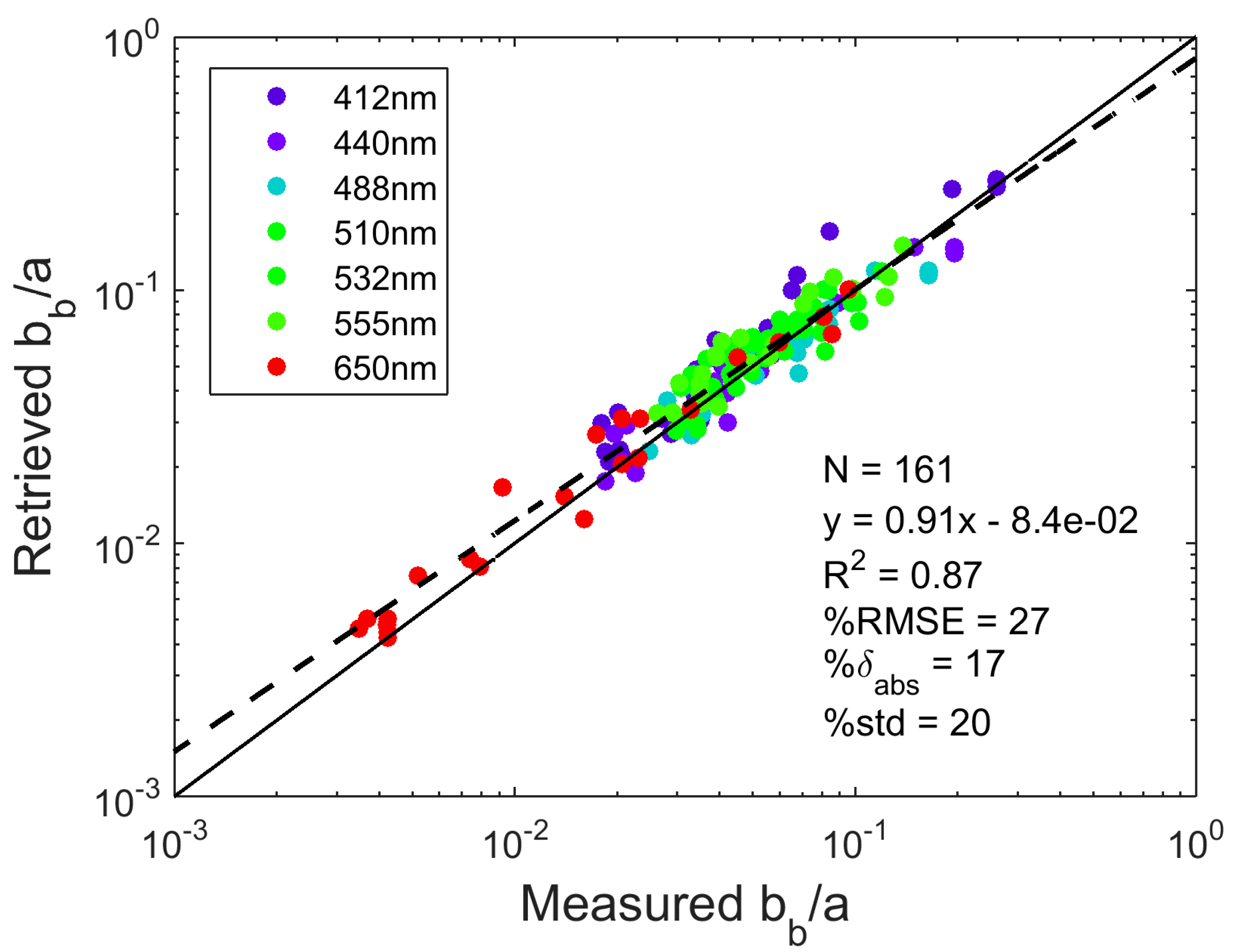
4.4. Assessment with Global NOMAD Data Set

Figure 6A shows results for the ZTT model applied to a subset of 80 measurements from the NASA NOMAD global data set. IOPs were averaged over the first optical depth. Match up MAPE %δ_abs of 20% was observed for this global data set, comparing favorably to the error of 16% observed with the high quality data set from Tonizzo et al. [29] (Table 1; see Table 2 for spectral breakdown). This is especially true considering the different IOP and r_rs processing approaches (e.g., there are several scattering error correction options for in-water absorption measurements) used for these data sets. If ${\tilde{b}}_{bp}$ is constrained to 0.006, MAPE %δ_abs increases to 23% (Figure 6B). Results from ZTT runs for other fixed ${\tilde{b}}_{bp}$ are shown in Table 1, where the dependency of performance on ${\tilde{b}}_{bp}$ is again apparent.

If the Morel et al. [7] approach for deriving the phase function from [Chl] is used as input into the ZTT model, %δ_abs increased from 20% to 26% for the NOMAD data (Table 1). If measured ${\tilde{b}}_{bp}$ are used to derive P_bb,FF(ψ,${\tilde{b}}_{bp}$) following [67], %δ_abs increased to 25% for the ZTT model.

Match ups are also shown for implementation of the full M02 and L11 models with the NOMAD data set (Figure 6C,D). MAPE statistics are summarized in Table 1 and Table 2. There are several possibilities for the systematically lower measured r_rs in the red spectral region for these data: (1) Suboptimal surface extrapolation of radiances due to water Raman effects [80,81], (2) residual scattering errors in reported in-water absorption measurements that may promote a bias to higher values of modeled r_rs (e.g., [29,49]), and/or (3) suboptimal corrections for sensor self-shading, which can be strong in clear water at longer wavelengths due to water absorption [82,83].

5. Discussion

The ZTT analytical model for remote sensing reflectance is based on the restatement of the RT equation by Zaneveld [27,28] with the following refinements: (1) Full bidirectionality was retained in the final model (no assumption of nadir viewing), (2) the assumption of asymptotic diffuse attenuation for upwelling radiances at the surface was analytically described, (3) the entire model was formulated in terms of b_b and a to enable inversion, (4) the VSF was explicitly included with β_p(ψ)/b_bp set to a constant shape defined by P_bb,ST(ψ) [26], which showed the strongest performance of any phase function, including measured phase functions in disparate, diverse data sets, (5) water Raman effects were added, and (6) for r_rs, an analytical model for ${\overline{\mu }}_d$ was developed that included dependency on atmospheric visibility. IOP inputs to the ZTT model are b_bp, a_pg, β_p(ψ)/b_bp, and ${\tilde{b}}_{bp}$. Moreover, the ZTT model enables systematic assessment of the effect of IOPs on the BRDF for the first time.

ZTT showed strong performance in match ups with field data sets spanning a wide range of water types. In terms of MAPE, the model with constant phase function shape P_bb,ST(ψ) performed as well as full RT computations. Stronger performance was observed for these available data sets relative to current state-of-the-art LUT-configured models based on the first order approximation between r_rs and b_b/a or b_b/(a + b_b), i.e., M02 and L11.

MAPE for the ZTT model was slightly better using P_bb,ST(ψ) (%δ_abs of 16%) when compared to using directly measured backward phase functions for the validation data set (where %δ_abs was 17%). It may be argued, under certain conditions, the broad average P_bb,ST(ψ) may be more accurate than an isolated measurement because specific bias errors in any single VSF measurement at an individual angle may be avoided. This of course assumes such biases may be larger than the natural variability in the shape of the backward phase function. Another explanation is error assessments for the validation data set were made over a relatively few number of stations, 23. To roughly estimate uncertainty in this error metric, single stations were sequentially left out of the error determination for ZTT using P_bb,ST(ψ), which gave a total range in %δ_abs of 14.8 to 16.8% with standard deviation of 0.6%. A ~1% difference in error may thus not be particularly meaningful.

The ZTT model is fully analytical in the sense it is described entirely by equations and “almost fully analytical” with respect to the inclusion of empiricism. Empiricism comes from optimizing the f_L parameter to our synthetic data set based on [Chl]-based bio-optical models, with MAPE improving by a significant ~3% compared to setting f_L equal to a spectrally constant 1.05. Using the constant P_bb,ST(ψ) backward phase function shape also introduced empiricism. If sample-specific Fournier-Forand analytical phase functions, based on ${\tilde{b}}_{bp}$ were used, errors in the validation data set increased by 3–5% (Table 1).

Particulate phase function shapes from Morel et al. [7] were modeled using the T-matrix approach, assuming homogeneous spheroidal shapes with constant n_p of 1.06. Although the endmember phase function shapes were not consistent with P_bb,ST(ψ) and P_bb,FF(ψ,${\tilde{b}}_{bp}$) shapes, many of the blended phase functions were. If P_bb,ST(ψ) may be considered widely representative, increasing errors may be expected in applying the M02 model to the lowest and highest Chl conditions where the endmember phase functions would fully manifest. Phase functions in the Chl range 1 to 10 mg m⁻³ were in closest agreement to P_bb,ST(ψ). Applying phase functions derived using the Morel et al. [7] approach in the ZTT model increased errors relative to using a constant P_bb,ST(ψ) by a significant 7% for the validation data set of [29] (from 16% to 23%) (Table 1). This error was also larger than the 21% error observed for M02 (addressed further below).

Since L11 used a Fournier-Forand phase function where ${\tilde{b}}_{bp}=1\%$ and the average Petzold phase function as endmembers [shown in 26, their Figure 3], many blended shapes from L11 should be relatively similar in the backward to the P_bb,ST(ψ) used in ZTT (although the Petzold shape does exhibit systematic discrepancies). This particular P_bb,FF with ${\tilde{b}}_{bp}$ = 1% is actually a very close match to P_bb,ST. L11 was developed through least-squares fitting with respect to Hydrolight results, so all the blended phase functions are weighted in the results.

A “typical marine atmosphere” and associated incident sky radiance distribution were used in the Hydrolight RT computations for the synthetic data set, the effects of which enter the ZTT model through spectral optimization of the upwelling radiance shape factor f_L (Section 4.1). The parameters ${\Psi }_{K_{Lu}}$ and ${\overline{\mu }}_{\infty }$ were also solved with Hydrolight RT simulations assuming the same atmosphere. The M02 and L11 models also assumed a single “typical marine atmosphere” in their simulations using Hydrolight based on Reference [58], so this aspect of the models should be consistent. The ${\overline{\mu }}_d$ term in the ZTT model has added flexibility in accommodating varying atmospheric visibility (closely related to AOT; [58]) inasmuch as V is an explicit term for ${\overline{\mu }}_d$.

One question arising from this work is, if the phase function shape P_bb,ST may indeed be considered highly representative, how would a LUT-based model following the approach of M02 but using P_bb,ST perform? To test this, we developed a LUT based on the first order r_rs proportionality to b_b/a, using the synthetic data set described in Section 3.1. The particle phase function was constant, consisting of P_bb,ST in the backward and a Fournier-Forand phase function with ${\tilde{b}}_{bp}$ = 0.006 for the forward direction (this had the best performance for the ZTT model in the validation data set [29], with MAPE = 17%). The LUT approach resulted in a MAPE of 22% for the validation data set and 26% for the NOMAD data. This performance is very close to M02 (21% and 25%, respectively) and L11 (21% and 26%, respectively). An insight we can take from this analysis is that a component, such as phase function shape in the different models cannot be considered in a vacuum, i.e., each model has a large set of assumptions that ultimately influence final performance. Furthermore, although not always explicitly stated in the literature, field validation efforts are likely to have had a role in updating assumptions through the course of development and testing of some models to ensure the model was well aligned with available data. For example, in our case, the f_L expression (Section 4.1) was developed from an assumed synthetic data set and the ${\tilde{b}}_{bp}$ value of 0.006 was recommended as it ultimately provided the best results with the field validation data sets available.

Recent work by Zhang et al. [84] has suggested the possibility of substantial variability in phase function shape in the backward direction, including up to a 40% increase for β_p(ψ)/b_bp in the near backward relative to β_p(120°)/b_bp. These results are in stark contrast to the comprehensive study of [26] and other published phase functions in the literature (e.g., [35,85]). Other recent works showing increases in the VSF at ψ > 150° [86,87,88] were made in enclosed cuvettes and did not include any correction for internal reflections (e.g., [89]), which are typically a difficult problem in laboratory VSF devices, since the scattered signal in the backward direction is orders of magnitude smaller than the forward. The Zhang et al. [84] results are also inconsistent with the phase functions used in previous BRDF models, such as M02, which have been shown to have satisfactory performance in validation efforts [17,18], even in many Case II coastal waters [19,90]. The recent theoretical r_rs modeling study of Xiong et al. [91] based on the phase function shapes presented in [84], where up to 50% disagreement with L11 was observed, consequently appear unrealistic.

Calibration and possible bias errors in the VSF device MASCOT used in [26] to derive P_bb,ST(ψ) have been evaluated in detail [36,48]. The MASCOT is an open path, in situ device with 17 independently calibrated detectors resolving the VSF from 10° to 170° in 10° increments. There are two calibration coefficients for each channel, a dark offset (obtained with the source occluded) and a scaling factor to convert digital counts to VSF units m⁻¹ sr⁻¹. Moreover, the observation of a remarkably consistent shape in the backward phase function for VSFs spanning more than four orders of magnitude in dynamic range cannot be explained by any known bias error in these coefficients. In fact this observation argues against any systematic bias, as consistency in phase function shapes during serial particle suspension experiments is a useful method to assess the accuracy of calibrations.

Recently, He et al. [20] developed a BRDF model also based on Zaneveld [28] but it differs from our implementation is several ways: (1) only the BRDF aspect was considered; (2) one wavelength was considered; (3) the formulation was in terms of a LUT (similar to M02 and L11) for aggregated terms; (4) widely varying backward phase function shapes were assumed after [84] described above; (5) the ${\overline{\mu }}_d$ model depended only on “typical average” sky conditions; and (6) water Raman effects were excluded. Direct comparisons were thus not possible here.

5.1. Assessing Residual Bias in the Model

The assumption of single scattering in the simplification of f_b (Section 2, Equation (2)) is not expected to invoke significant errors at turbidity levels found for most oceanic and coastal waters [5,13]. As shown by Gordon [23], secondary scattering events for light redirected toward the backward direction, i.e., downwelling radiance scattered into the upwelling radiance field, has a negligible effect on the shape of the upwelling radiance distribution because the vast majority of these scattering events are in the near forward direction. The full effects of multiple scattering were included in relationships for other terms in the model as they were determined using full RT modeling.

MASCOT VSF measurements used to determine P_bb,ST(ψ) only extended to 170°, so the application of this function for ψ > 170° in the model is uncertain. There were no ψ > 170° in the data sets tested here, although such scattering angles may be expected for some viewing geometries for the PACE imager (Figure 1). There is a need for a better understanding of phase function shapes for ψ > 170° and this extends to other applications, such as lidar [92].

Only nadir viewing was considered for the analytical relationships for $K_{Lu}$ and f_L and we suggest these relationships may be transferable to other viewing geometries as long as ψ is preserved. This assumption has been verified in Hydrolight simulations to have small errors for representative cases, but cannot be assessed with the field data sets available here, which all have nadir viewing. This is being considered in future work, and, moreover, emphasizes the need for routine measurements of full upwelling radiance distributions in ocean color validation work as validation only with nadir radiance L_u(θ_s,θ_v = π) neglects the BRDF effects that are essential to any algorithm.

The optimization of f_L was based on the [Chl]-based synthetic data set. A significant deviation from the bio-optical model assumptions of that synthetic data set could lead to a discrepancy in match ups, however it worth pointing out (1) f_L has a relatively weak dependency on IOPs except for the VSF shape in the backward direction (which is effectively accounted for in the solar zenith dependency in Equation (30)), and (2) other state-of-the-art models (i.e., M02 and L11) are constructed entirely around such synthetic data sets. A benefit of the ZTT model is that an analytical relationship for a specific term of the model may be replaced later if a more optimal approach is demonstrated.

As shown in Zaneveld [27,28], L_u normalized to E_od is more closely linked to the RT Equation than L_u/E_d, where an additional ${\overline{\mu }}_d$ term must be added to the model (Section 2.6). Adding this term is expected to increase uncertainty in the RT model and inversion. Scalar irradiance has the additional advantage of being less dependent on solar zenith angle and sky radiance distributions. As discussed in Section 2.6, sensor technology is available to measure E_od and inclusion of these measurements in field efforts focused on algorithm development and validation should be encouraged. When the ${\overline{\mu }}_d$ term must be included in association with E_d measurements, AOT is also a useful validation measurement that may be made in the field [93] and used to derive visibility V [58] for input in Equation (16) or full RT computations.

Lastly, potential uncertainties in the full RT computations must be considered, as this was used to parameterize several ZTT terms. Polarization is not considered in the ZTT model or in Hydrolight, which is likely important [29,33]. There is a need in the research community for commercially available RT code with a focus on the ocean that includes full polarization, along with concomitant measurements of polarized radiance in the field. Neither the Hydrolight simulations or ZTT model included inelastic effects from DOM fluorescence, which could lead to bias errors as high as about 10% in the mid-visible [33]. Another potential source of uncertainty is the water Raman estimation [60], where bias errors as high as 10% can be typical.

5.2. Suitability for Inversion

The ZTT model can be used to directly solve for b_b/a using least-squares minimization of a r_rs measurement at any wavelength. This is shown in Figure 7 for the validation data set from Tonizzo et al. [29], assuming a constant ${\tilde{b}}_{bp}$ of 0.006. The typical value for V of 15 km was assumed. MAPE %δ_abs in the inversion was 17%, which matches results from full RT simulations of closure in the forward direction. Residual errors thus appear almost entirely comprised of the inherent errors of the data set arising from IOP and radiometric measurements [29]. With respect to the use of P_bb,ST(ψ), another potential approach to estimating VSF shape as it relates to the upcoming PACE mission is using planned multi- and hyper-angular polarimetry data from the Hyper-Angular Rainbow Polarimeter-2 (HARP2; contributed by University of Maryland, Baltimore County) and the Spectrometer for Planetary Exploration—one (SPEXone; contributed by the Netherlands Institute for Space Research) [94]. If information on the backward shape of the VSF could be gleaned with sufficient accuracy from angular polarimetry data (only a few angles would be necessary), this could be used directly in the ZTT model.

The ZTT model described here only addresses in-water RT, although the current approach to normalize water-leaving radiances measured by a satellite imager is expected to directly apply (see [15], Sections 3.1 and 6]). The BRDF is built-in to the Zaneveld model so an additional step to conceptually shift the geometry to a normalized geometry standard would not be required for IOP inversion. A normalized geometry (to nadir viewing or other geometry) could still be applied to intercompare reflectances in images. Translation to water-leaving radiance by accounting for all the reflection and refraction effects through the air-sea interface i.e., $ℛ$(θ_s,θ_v) in [6,15], can still be applied. Similarly, the effects of varying Earth-Sun distance and atmospheric attenuation can be removed following the current approach. Moreover, we would expect a practical implementation of this analytical model to have similar computational requirements as the current M02 LUT-based approach.

The ZTT model shows ${\tilde{b}}_{bp}$ exerts some influence on r_rs (Table 1) and the potential to invert r_rs for ${\tilde{b}}_{bp}$ is also being investigated. The parameter ${\tilde{b}}_{bp}$ has not historically been associated with r_rs and could provide new insights into particle composition in natural waters (e.g., [41]). Even a retrieval of ${\tilde{b}}_{bp}$ with relatively large errors could be useful for many research applications.

The ZTT model is fully spectral and can be applied over the full anticipated ocean color hyperspectral wavelength range for the future PACE mission (350–800 nm). A primary goal in model development was parameterization entirely in terms of a and b_b. Inversion approaches, such as the General IOP (GIOP) inversion using a least-squares minimization to solve for IOP subcomponents [16] may consequently be readily applied. Spectral b_bp and a_pg can be solved using assumptions for subcomponent IOP spectra through least squares minimization of Equation (18). This is the step where empiricism prominently enters the problem as spectral shapes for IOP subcomponents must be assumed. This is being examined in ongoing work. Further investigation is needed to determine IOP subcomponent spectra with a high spectral resolution for error minimization over this full spectral range in inversion, which is currently being assessed by the PACE Science Team [13,95]. Hyperspectral (i.e., 5 nm) resolution for PACE is expected to improve fidelity in inverting for subcomponents (and potentially ${\tilde{b}}_{bp}$) as there will be higher degrees of freedom than for multi-spectral imagers [96,97].

Code for the ZTT model in MATLAB is available at ioccg.org.

References

1. Gordon, H.R. Inverse methods in hydrologic optics. Oceanologia 2002, 44, 9–58. [Google Scholar]
2. Zaneveld, J.R.V.; Twardowski, M.S.; Lewis, M.; Barnard, A. Radiative transfer and remote sensing. In Remote Sensing of Coastal Aquatic Waters; Miller, R., Del-Castillo, C., McKee, B., Eds.; Springer: Dordrecht, The Netherlands, 2005; pp. 1–20. [Google Scholar]
3. Twardowski, M.; Lewis, M.; Barnard, A.; Zaneveld, J.R.V. In-water instrumentation and platforms for ocean color remote sensing applications. In Remote Sensing of Coastal Aquatic Waters; Miller, R., Del-Castillo, C., McKee, B., Eds.; Springer: Dordrecht, The Netherlands, 2005; pp. 69–100. [Google Scholar]
4. Mobley, C.D. Light and Water: Radiative Transfer in Natural Waters; Academic Press: San Diego, CA, USA, 1994; 592p. [Google Scholar]
5. Morel, A.; Gentili, B. Diffuse reflectance of oceanic waters. II. Bidirectional aspects. Appl. Opt. 1993, 32, 6864–6879. [Google Scholar] [CrossRef] [PubMed]
6. Morel, A.; Gentili, B. Diffuse reflectance of oceanic waters. III. Implication of bidirectionality for the remote-sensing problem. Appl. Opt. 1996, 35, 4850. [Google Scholar] [CrossRef] [PubMed]
7. Morel, A.; Antoine, D.; Gentili, B. Bidirectional reflectance of oceanic waters: Accounting for Raman emission and varying particle phase function. Appl. Opt. 2002, 41, 6289–6306. [Google Scholar] [CrossRef] [PubMed]
8. Fan, Y.; Li, W.; Gatebe, C.K.; Stamnes, K. Neural network method to correct bidirectional effects in water leaving radiance. Appl. Opt. 2016, 55, 10–21. [Google Scholar] [CrossRef] [PubMed]
9. Gordon, H.; Brown, O.B.; Evans, R.H.; Brown, J.W.; Smith, R.C.; Baker, K.S.; Clark, D.K. A semianalytic radiance model of ocean color. J. Geophys. Res. 1988, 93, 10909–10924. [Google Scholar] [CrossRef]
10. Park, Y.-J.; Ruddick, K. Model of remote sensing reflectance including bidirectional effects for case 1 and case 2 waters. Appl. Opt. 2005, 44, 1236–1249. [Google Scholar] [CrossRef]
11. Lee, Z.-P.; Du, K.-P.; Voss, K.J.; Zibordi, G.; Lubac, B.; Arnone, R.; Weidemann, A. An inherent optical property centered approach to correct the angular effects in water-leaving radiance. Appl. Opt. 2011, 50, 3155–3167. [Google Scholar] [CrossRef]
12. Hlaing, S.; Gilerson, A.; Harmel, T.; Tonizzo, A.; Weidemann, A.; Arnone, R.; Ahmed, S. Assessment of a bidirectional reflectance distribution correction of above-water and satellite water-leaving radiance in coastal waters. Appl. Opt. 2012, 51, 220–237. [Google Scholar] [CrossRef]
13. Werdell, J.; McKinna, L.I.W.; Boss, E.; Ackleson, S.G.; Craig, S.E.; Gregg, W.W.; Lee, Z.-P.; Maritorena, S.; Roesler, C.S.; Rousseaux, C.S.; et al. An overview of approaches and challenges for retrieving marine inherent optical properties from ocean color remote sensing. Prog. Oceanogr. 2018, 160, 186–212. [Google Scholar] [CrossRef]
14. Morel, A. In-water and remote measurements of ocean color. Bound.-Lay. Meteorl. 1980, 18, 177–201. [Google Scholar] [CrossRef]
15. Mobley, C.D.; Werdell, J.; Franz, B.; Ahmad, Z.; Bailey, S. Atmospheric Correction for Satellite Ocean Color Radiometry; NASA Report NASA/TM–2016-217551; NASA: Washington, DC, USA, 2016; 73p.
16. Werdell, P.J.; Franz, B.A.; Bailey, S.W.; Feldman, G.C.; Boss, E.; Brando, V.E.; Dowell, M.; Hirata, T.; Lavender, S.J.; Lee, Z.-P.; et al. Generalized ocean color inversion model for retrieving marine inherent optical properties. Appl. Opt. 2013, 52, 2019–2037. [Google Scholar] [CrossRef] [PubMed] [Green Version]
17. Voss, K.; Morel, A. Bidirectional reflectance function for oceanic waters with varying chlorophyll concentrations: Measurements versus predictions. Limnol. Oceanogr. 2005, 50, 698–705. [Google Scholar] [CrossRef] [Green Version]
18. Voss, K.J.; Morel, A.; Antoine, D. Detailed validation of the bidirectional effect in various Case 1 waters for application to ocean color imagery. Biogeosciences 2007, 4, 781–789. [Google Scholar] [CrossRef] [Green Version]
19. Gleason, A.; Voss, K.; Gordon, H.R.; Twardowski, M.; Sullivan, J.; Trees, C.; Weidemann, A.; Berthon, J.-F.; Clark, D.; Lee, Z.-P. Detailed validation of ocean color bidirectional effects in various Case I and Case II waters. Opt. Express 2012, 20, 7630–7645. [Google Scholar] [CrossRef]
20. He, S.; Zhang, X.; Xiong, Y.; Gray, D. A bidirectional subsurface remote sensing reflectance model explicitly accounting for particle backscattering shapes. J. Geophys. Res. Oceans 2017, 122, 8614–8626. [Google Scholar] [CrossRef]
21. Talone, M.; Zibordi, G.; Lee, Z.-P. Correction for the non-nadir viewing geometry of AERONET-OC above water radiometry data: An estimate of uncertainties. Opt. Express 2018, 26, A541–A561. [Google Scholar] [CrossRef] [PubMed]
22. Hirata, T.; Hardman-Mountford, N.; Aiken, J.; Fishwick, J. Relationship between the distribution function of ocean nadir radiance and inherent optical properties for oceanic waters. Appl. Opt. 2009, 48, 3129–3138. [Google Scholar] [CrossRef] [PubMed]
23. Gordon, H.R. Sensitivity of radiative transfer to small-angle scattering in the ocean: Quantitative assessment. Appl. Opt. 1993, 32, 7505–7511. [Google Scholar] [CrossRef] [PubMed]
24. Mishchenko, M.I.; Travis, L.D.; Lacis, A.A. Scattering, Absorption, and Emission of Light by Small Particles; Cambridge University Press: Cambridge, UK, 2002; pp. 74–82. [Google Scholar]
25. Hair, J.; Hostetler, C.; Hu, Y.; Behrenfeld, M.; Butler, C.F.; Harper, D.B.; Hare, R.; Berkoff, R.; Cook, A.; Collins, J.; et al. Combined Atmospheric and Ocean Profiling from an Airborne High Spectral Resolution Lidar. Eur. Phys. J. Conf. 2016, 119, 22001. [Google Scholar] [CrossRef] [Green Version]
26. Sullivan, J.M.; Twardowski, M.S. Angular shape of the volume scattering function in the backward direction. Appl. Opt. 2009, 48, 6811–6819. [Google Scholar] [CrossRef] [PubMed]
27. Zaneveld, J.R.V. Remotely sensed reflectance and its dependence on vertical structure: A theoretical derivation. Appl. Opt. 1982, 21, 4146–4150. [Google Scholar] [PubMed]
28. Zaneveld, J.R.V. A theoretical derivation of the dependence of the remotely sensed reflectance on the inherent optical properties. J. Geophys. Res. 1995, 100, 13135–13142. [Google Scholar] [CrossRef]
29. Tonizzo, A.; Twardowski, M.; McLean, S.; Voss, K.; Lewis, M.; Trees, C. Closure and uncertainty assessment for ocean color reflectance using measured volume scattering functions and reflective tube absorption coefficients with novel correction for scattering. Appl. Opt. 2017, 56, 130–146. [Google Scholar] [CrossRef]
30. Wolanin, A.; Rozanov, V.; Dinter, T.; Bracher, A. Detecting CDOM Fluorescence Using High Spectrally Resolved Satellite Data: A Model Study. In Towards an Interdisciplinary Approach in Earth System Science: Advances of a Helmholtz Graduate Research School; Springer International Publishing: Cham, Switzerland, 2015; pp. 109–121. [Google Scholar] [Green Version]
31. Zhai, P.W.; Hu, Y.; Winker, D.M.; Franz, B.A.; Boss, E. Contribution of Raman scattering to polarized radiation field in ocean waters. Opt. Express 2015, 23, 23582–23596. [Google Scholar] [CrossRef]
32. Rozanov, V.; Dinter, T.; Rozanov, A.; Wolanin, A.; Bracher, A.; Burrows, J. Radiative transfer modeling through terrestrial atmosphere and ocean accounting for inelastic processes: Software package SCIATRAN. J. Quant. Spectrosc. Radiat. Transf. 2017, 194, 65–85. [Google Scholar] [CrossRef] [Green Version]
33. Zhai, P.W.; Hu, Y.; Winker, D.M.; Franz, B.A.; Werdell, J.; Boss, E. Vector radiative transfer model for coupled atmosphere and ocean systems including inelastic sources in ocean waters. Opt. Express 2017, 25, A223–A239. [Google Scholar] [CrossRef]
34. Weidemann, A.; Stavn, R.; Zaneveld, J.R.V.; Wilcox, M.R. Error in predicting hydrosol backscattering from remotely sensed reflectance. J. Geophys. Res. 1995, 100, 163–177. [Google Scholar] [CrossRef]
35. Berthon, J.-F.; Shybanov, E.; Lee, M.; Zibordi, G. Measurements and modeling of the volume scattering function in the coastal northern Adriatic Sea. Appl. Opt. 2007, 46, 5189–5203. [Google Scholar] [CrossRef]
36. Twardowski, M.; Zhang, X.; Vagle, S.; Sullivan, J.; Freeman, S.; Czerski, H.; You, Y.; Bi, L.; Kattawar, G. The optical volume scattering function in a surf zone inverted to derive sediment and bubble particle subpopulations. J. Geophys. Res. 2012, 117, C00H17. [Google Scholar] [CrossRef]
37. Lee, M.; Korchemkina, E.N. Chapter 4: Volume scattering function of seawater. In Springer Series in Light Scattering; Kokhanovsky, A., Ed.; Springer International Publishing: New York, NY, USA, 2017; pp. 151–195. [Google Scholar]
38. Voss, K.; Austin, R. Beam attenuation measurement error due to small angle scattering acceptance. J. Atmos. Ocean. Technol. 1993, 10, 113–121. [Google Scholar] [CrossRef]
39. Boss, E.; Slade, W.H.; Behrenfeld, M.; Dall’Olmo, G. Acceptance angle effects on the beam attenuation in the ocean. Opt. Express 2009, 17, 1535–1550. [Google Scholar] [CrossRef] [PubMed]
40. Twardowski, M.; Tonizzo, A. Scattering and absorption effects on asymptotic light fields in seawater. Opt. Express 2017, 25, 18122–18130. [Google Scholar] [CrossRef] [PubMed]
41. Twardowski, M.S.; Boss, E.; Macdonald, J.B.; Pegau, W.S.; Barnard, A.H.; Zaneveld, J.R.V. A model for estimating bulk refractive index from the optical backscattering ratio and the implications for understanding particle composition in Case I and Case II waters. J. Geophys. Res. 2001, 106, 14129–14142. [Google Scholar] [CrossRef]
42. Prieur, L.; Morel, A. Etude theorique du regime asymptotique: Relations entre characteristiques optiques et coefficient d’extinction relatif a la penetration de la lumibr, e du jour. Cah. Oceanogr. 1971, 23, 35–48. [Google Scholar]
43. Berwald, J.; Stramski, D.; Mobley, C.D.; Kiefer, D.A. Influences of absorption and scattering on vertical changes in the average cosine of the underwater light field. Limnol. Oceanogr. 1995, 40, 1347–1357. [Google Scholar] [CrossRef] [Green Version]
44. Fournier, G.; Forand, F. Analytic phase function for ocean water. Ocean Opt. XII 1994, 2558, 194–201. [Google Scholar]
45. Jonasz, M.; Fournier, G. Light Scattering by Particles in Water; Academic Press: Amsterdam, The Netherlands, 2007; 704p. [Google Scholar]
46. IOCCG. Remote Sensing of Inherent Optical Properties: Fundamentals, Tests of Algorithms, and Applications. In Reports of the International Ocean-Colour Coordinating Group, No. 5; Lee, Z.-P., Ed.; IOCCG: Dartmouth, NS, Canada, 2006; 123p. [Google Scholar]
47. Twardowski, M.S.; Sullivan, J.M.; Donaghay, P.L.; Zaneveld, J.R.V. Microscale quantification of the absorption by dissolved and particulate material in coastal waters with an ac-9. J. Atmos. Ocean. Technol. 1999, 16, 691–707. [Google Scholar] [CrossRef]
48. Sullivan, J.; Twardowski, M.; Zaneveld, J.R.V.; Moore, C. Measuring optical backscattering in water. In Light Scattering Reviews 7: Radiative Transfer and Optical Properties of Atmosphere and Underlying Surface; Kokhanovsky, A., Ed.; Springer Praxis Books: New York, NY, USA; pp. 189–224. [CrossRef]
49. Stockley, N.D.; Rottgers, R.; McKee, D.; Lefering, I.; Sullivan, J.M.; Twardowski, M.S. Assessing uncertainties in scattering correction algorithms for reflective tube absorption measurements made with a WET Labs ac-9. Opt. Express 2017, 25, A1139–A1153. [Google Scholar] [CrossRef]
50. Gordon, H.R.; Brown, O.B.; Jacobs, M.M. Computed relationships between the inherent and apparent optical properties of a flat homogeneous ocean. Appl. Opt. 1975, 14, 417–427. [Google Scholar] [CrossRef] [PubMed]
51. Twardowski, M.S.; Claustre, H.; Freeman, S.A.; Stramski, D.; Huot, Y. Optical backscattering properties of the “clearest” natural waters. Biogeosciences 2007, 4, 1041–1058. [Google Scholar] [CrossRef]
52. Zhang, X.D.; Hu, L.B.; He, M.-X. Scattering by pure seawater: Effect of salinity. Opt. Express 2009, 17, 5698–5710. [Google Scholar] [CrossRef] [PubMed]
53. Twardowski, M.; Jamet, C.; Loisel, H. Analytical Model to Derive Suspended Particulate Matter Concentration in Natural Waters by Inversion of Optical Attenuation and Backscattering. Proc. SPIE Ocean Sens. Monit. X 2018. [Google Scholar] [CrossRef]
54. Boss, E.; Pegau, W.S.; Lee, M.; Twardowski, M.S.; Shybanov, E.; Korotaev, G.; Baratange, F. The particulate backscattering ratio at LEO 15 and its use to study particles composition and distribution. J. Geophys. Res. 2004, 109, C01014. [Google Scholar] [CrossRef]
55. Sullivan, J.M.; Twardowski, M.S.; Donaghay, P.L.; Freeman, S.A. Using scattering characteristics to discriminate particle types in US coastal waters. Appl. Opt. 2005, 44, 1667–1680. [Google Scholar] [CrossRef] [PubMed]
56. Stramski, D.; Reynolds, R.A.; Babin, M.; Kaczmarek, S.; Lewis, M.R.; Röttgers, R.; Sciandra, A.; Stramska, M.; Twardowski, M.S.; Franz, B.A.; et al. Relationships between the surface concentration of particulate organic carbon and optical properties in the eastern South Pacific and eastern Atlantic Oceans. Biogeosciences 2008, 5, 171–201. [Google Scholar] [CrossRef] [Green Version]
57. Morel, A.; Prieur, L. Analyse spectrale des coefficients d’attenuation diffuse, de retrodiffusion pour diverses regions marines. Cent. Rech. Oceanogr. 1975, 17, 1–157. [Google Scholar]
58. Gregg, W.; Carder, K. A simple spectral solar irradiance model for cloudless maritime atmospheres. Limnol. Oceanogr. 1990, 35, 1657–1675. [Google Scholar] [CrossRef] [Green Version]
59. Loisel, H.; Stramski, D. Estimation of the inherent optical properties of natural waters from the irradiance attenuation coefficient and reflectance in the presence of Raman scattering. Appl. Opt. 2000, 39, 3001–3011. [Google Scholar] [CrossRef]
60. Westberry, T.K.; Boss, W.; Lee, Z.-P. Influence of Raman scattering on ocean color inversion models. Appl. Opt. 2013, 52, 5552–5561. [Google Scholar] [CrossRef]
61. Pope, R.M.; Fry, E. Absorption spectrum (380–700 nm) of pure water. II. Integrating cavity measurements. Appl. Opt. 1997, 36, 8710–8723. [Google Scholar] [CrossRef]
62. Ciotti, A.M.; Lewis, M.R.; Cullen, J.J. Assessment of the relationships between dominant cell size in natural phytoplankton communities and the spectral shape of the absorption coefficient. Limnol. Oceanogr. 2002, 47, 404–417. [Google Scholar] [CrossRef] [Green Version]
63. Roesler, C.S.; Perry, M.J. In situ phytoplankton absorption, fluorescence emission, and particulate backscattering spectra determined from reflectance. J. Geophys. Res. 1995, 100, 13279–13294. [Google Scholar] [CrossRef]
64. Twardowski, M.S.; Boss, E.; Sullivan, J.M.; Donaghay, P.L. Modeling the spectral shape of absorbing chromophoric dissolved organic matter. Mar. Chem. 2004, 89, 69–88. [Google Scholar] [CrossRef]
65. Loisel, H.; Morel, A. Light scattering and chlorophyll concentration in case 1 waters: A reexamination. Limnol. Oceanogr. 1998, 43, 847–858. [Google Scholar] [CrossRef] [Green Version]
66. Morel, A. Are the empirical relationships describing the bio-optical properties of case 1 waters consistent and internally compatible? J. Geophys. Res. 2009, 114, C01016. [Google Scholar] [CrossRef]
67. Mobley, C.D.; Sundman, L.K.; Boss, E. Phase function effects on oceanic light fields. Appl. Opt. 2002, 41, 1035–1050. [Google Scholar] [CrossRef] [PubMed]
68. Voss, K.J.; McLean, S.; Lewis, M.; Johnson, C.; Flora, S.; Feinholz, M.; Yarbrough, M.; Trees, C.; Twardowski, M.; Clark, D. An example crossover experiment for testing new vicarious calibration techniques for satellite ocean color radiometry. J. Atmos. Ocean. Technol. 2010, 27, 1747–1759. [Google Scholar] [CrossRef]
69. Zaneveld, J.R.V.; Barnard, A.H.; Boss, E. A theoretical derivation of the depth average of remotely sensed optical parameters. Opt. Express 2005, 13, 9052–9061. [Google Scholar] [CrossRef]
70. Gordon, H.R.; Clark, D.K. Remote sensing optical properties of a stratified ocean: An improved interpretation. Appl. Opt. 1980, 19, 3428–3430. [Google Scholar] [CrossRef]
71. Gordon, H.R. Dependence of the diffuse reflectance of natural waters on the sun angle. Limnol. Oceanogr. 1989, 34, 1484. [Google Scholar] [CrossRef]
72. Kirk, J.T.O. Estimation of the absorption and scattering coefficients of natural waters by the use of underwater irradiance measurements. Appl. Opt. 1994, 33, 3276–3278. [Google Scholar] [CrossRef] [PubMed]
73. Lee, Z.-P.; Du, K.-P.; Arnone, R. A model for the diffuse attenuation coefficient of downwelling irradiance. J. Geophys. Res. 2005, 110, C02016. [Google Scholar] [CrossRef]
74. Chai, T.; Draxler, R.R. Root mean square error (RMSE) or mean absolute error (MAE)?—Arguments against avoiding RMSE in the literature. Geosci. Model. Dev. 2014, 7, 1247–1250. [Google Scholar] [CrossRef]
75. Brewin, R.J.W. The Ocean Colour Climate Change Initiative: III. A round-robin comparison on in-water bio-optical algorithms. Remote Sens. Environ. 2013. [Google Scholar] [CrossRef]
76. Hoge, F.; Lyon, P.E.; Mobley, C.D.; Sundman, L.K. Radiative transfer equation inversion: Theory and shape factor models for retrieval of oceanic inherent optical properties. J. Geophys. Res. 2003, 108, 3386. [Google Scholar] [CrossRef]
77. Agrawal, Y.; Mikkleson, O. Empirical forward scattering phase functions from 0.08 to 16 deg. for randomly shaped terrigenous 1-21 μm sediment grains. Opt. Express 2009, 17, 8805–14. [Google Scholar] [CrossRef] [PubMed]
78. Nardelli, S.; Twardowski, M.S. Improving assessments of chlorophyll concentration from in situ optical measurements. Opt. Express 2016, 24, A1374–A1389. [Google Scholar] [CrossRef] [PubMed]
79. Petzold, T.J. Volume Scattering Functions for Selected Ocean Waters, Report 72–78; Scripps Institution of Oceanography: La Jolla, CA, USA, 1972. [Google Scholar]
80. Li, L.; Stramski, D.; Reynolds, R.A. Effects of inelastic radiative processes on the determination of water-leaving spectral radiance from extrapolation of underwater near-surface measurements. Appl. Opt. 2016, 55, 7050–7067. [Google Scholar] [CrossRef]
81. Voss, K.; Gordon, H.; Flora, S.; Johnson, B.C.; Yarbrough, M.; Feinholz, M.; Houlihan, T. A method to extrapolate the diffuse upwelling radiance attenuation coefficient to the surface as applied to the Marine Optical Buoy (MOBY). J. Atmos. Ocean. Technol. 2017, 34, 1423–1432. [Google Scholar] [CrossRef]
82. Gordon, H.; Ding, K. Self-shading of in-water optical instruments. Limnol. Oceanogr. 1992, 37, 491–500. [Google Scholar] [CrossRef] [Green Version]
83. Leathers, R.A.; Downes, T.V.; Mobley, C.D. Self-shading correction for oceanographic upwelling radiometers. Opt. Express 2004, 12, 4709–4718. [Google Scholar] [CrossRef] [PubMed]
84. Zhang, X.; Fournier, G.R.; Gray, D.J. Interpretation of scattering by oceanic particles around 120 degrees and its implication in ocean color studies. Opt. Express 2017, 25, A191–A199. [Google Scholar] [CrossRef] [PubMed]
85. Lotsberg, J.K.; Marken, E.; Stamnes, J.; Erga, S.R.; Aursland, K.; Olseng, C. Laboratory measurements of light scattering from marine particles. Limnol. Oceanogr. Methods 2007, 5, 34–40. [Google Scholar] [CrossRef] [Green Version]
86. Tan, H.; Doerffer, R.; Oishi, T.; Tanaka, A. A new approach to measure the volume scattering function. Opt. Express 2013, 21, 18697–18711. [Google Scholar] [CrossRef] [PubMed]
87. Harmel, T.; Hieronymi, M.; Slade, W.; Röttgers, R.; Roullier, F.; Chami, M. Laboratory experiments for intercomparison of three volume scattering meters to measure angular scattering properties of hydrosols. Opt. Express 2016, 24, A234–A256. [Google Scholar] [CrossRef] [PubMed]
88. Tan, H.; Oishi, T.; Tanaka, A.; Doerffer, R.; Tan, Y. Chlorophyll-a specific volume scattering function of phytoplankton. Opt. Express 2017, 25, A564–A573. [Google Scholar] [CrossRef] [PubMed]
89. Volten, H.; de Haan, J.F.; Hovenier, J.W.; Schreurs, R.; Vassen, W.; Dekker, A.G.; Hoogenboom, H.J.; Charlton, F.; Wouts, R. Laboratory measurements of angular distributions of light scattered by phytoplankton and silt. Limnol. Oceanogr. 1998, 43, 1180–1197. [Google Scholar] [CrossRef] [Green Version]
90. Loisel, H.; Morel, A. Non-isotropy of the upward radiance field in typical coastal (Case 2) waters. Int. J. Remote Sens. 2001, 22, 275–295. [Google Scholar] [CrossRef]
91. Xiong, Y.; Zhang, X.; He, S.; Gray, D.J. Re-examining the effect of particle phase functions on the remote-sensing reflectance. Appl. Opt. 2017, 56, 6881–6888. [Google Scholar] [CrossRef]
92. Hostetler, C.; Behrenfeld, M.J.; Hu, Y.; Hair, J.W.; Schulien, J.A. Spaceborne lidar in the study of marine systems. Annu. Rev. Mar. Sci. 2018, 10, 121–147. [Google Scholar] [CrossRef]
93. Dayou, J.; Chang, J.H.W.; Sentian, J. Ground-Based Aerosol Optical Depth Measurement Using Sunphotometers; Springer: Singapore, 2014; pp. 9–30. [Google Scholar]
94. The NASA PACE Mission. Available online: https://pace.oceansciences.org/mission.htm (accessed on 16 June 2018).
95. Boss, E.; Remer, L.A. A novel approach to a satellite mission’s science team. Eos 2018, 99. [Google Scholar] [CrossRef]
96. Bracher, A.; Bouman, H.A.; Brewin, R.J.W.; Bricaud, A.; Brotas, V.; Ciotti, A.M.; Clementson, L.; Devred, E.; Di Cicco, A.; Dutkiewicz, S.; et al. Obtaining phytoplankton diversity from ocean color: A scientific roadmap for future development. Front. Mar. Sci. 2017, 4. [Google Scholar] [CrossRef]
97. Vandermeulen, R.A.; Mannino, A.; Neeley, A.; Werdell, J.; Arnone, R. Determining the optical spectral sampling frequency and uncertainty thresholds for hyperspectral remote sensing of ocean color. Opt. Express 2017, 25, A785–A797. [Google Scholar] [CrossRef] [PubMed]
Figure 1. Refracted, in-water scattering angles made between the solar zenith and viewing angle, simulated for the upcoming NASA PACE satellite imager through a complete polar orbit (solid blue). Scattering angle distributions for SeaWiFS were similar. Data courtesy Bryan Franz (NASA GSFC). Angular weighting functions of commercial backscattering sensors WET Labs ECO-BB, ECO-NTU, and MCOMS and IMO-SC6 (see text) are overlaid after scaling by 5 × 10⁶.
Applsci 08 02684 g001
Figure 2. Spectral dependency of the fL shape function at different θs’. Thin lines are solved fL functions for each θs′ for the synthetic data set and stars are from the model approximation with constant shape described by f L , a v e ( λ ) in Equation (30).
Applsci 08 02684 g002
Figure 3. rrs derived from the ZTT model with the synthetic data set compared to rrs simulated using Hydrolight (HL): (A) fL optimized spectrally (i.e., Equation (31) for the synthetic data set with Fournier-Forand phase functions individually determined for each [Chl]; (B) fL optimized spectrally for the synthetic data set with constant Pbb,ST(ψ) (see text); and (C) fL set to 1.05 with constant Pbb,ST(ψ). Colors represent wavelengths, from 400 to 700 nm with gray used for 350 < λ < 400 nm and 700 < λ < 800 nm.
Applsci 08 02684 g003
Figure 4. rrs computed from (A) ZTT, (B) ZTT with b ˜ b p fixed at 0.006, (C) M02, and (D) L11 models, compared to measured rrs in the high quality validation data set from Tonizzo et al. [29]. Note L11 does not account for Raman scattering. Chlorophyll input for M02 was derived from spectral absorption using the Nardelli and Twardowski [78] line height algorithm. MAPE %δabs was 16%, 17%, 21%, and 21%, in A through D, respectively.
Applsci 08 02684 g004
Figure 5. Phase functions in the backward direction used to assess the ZTT model. “ST2009” is Pbb,ST(ψ) from [26] with the assumption Pbb,ST(ψ > 170°) = Pbb,ST(170°); “Morel” is from Morel et al. [7] with endmember populations dominated by small and large particles also shown; “Measured” were directly measured; and “FF” are Fournier-Forand phase functions Pbb,FF(ψ, b ˜ b p ) derived from measured b ˜ b p following [67].
Applsci 08 02684 g005
Figure 6. As in Figure 4, but for the NASA NOMAD data set containing a, bb, rrs, and [Chl]. MAPE %δabs were 20%, 23%, 25%, and 26% in (AD), respectively.
Applsci 08 02684 g006
Figure 7. Comparing measured bb/a to results of inverting ZTT using least-squares minimization individually at each wavelength. Water Raman effects were removed before applying the ZTT model.
Applsci 08 02684 g007