Article

Optimal Irregular Wind Farm Design for Continuous Placement of Wind Turbines with a Two-Dimensional Jensen-Gaussian Wake Model

1
Research Center of Fluid Machinery Engineering and Technology, Jiangsu University, Zhenjiang 212013, China
2
School of Chemistry, Physics and Mechanical Engineering, Queensland University of Technology, Brisbane, QLD 4001, Australia
3
Department of Mechanical Engineering, University of Alberta, Edmonton, AB T6G 2R3, Canada
*
Author to whom correspondence should be addressed.
Appl. Sci. 2018, 8(12), 2660; https://doi.org/10.3390/app8122660
Submission received: 3 December 2018 / Accepted: 16 December 2018 / Published: 18 December 2018
(This article belongs to the Section Energy Science and Technology)

Abstract

:
Optimal design of wind turbine placement in a wind farm is one of the most effective tools to reduce wake power losses by alleviating the wake effect in the wind farm. In comparison to the discrete grid-based wind farm design method, the continuous coordinate method has the property of continuously varying the placement of wind turbines, and hence, is far more capable of obtaining the global optimum solutions. In this paper, the coordinate method was applied to optimize the layout of a real offshore wind farm for both simplified and realistic wind conditions. A new analytical wake model (Jensen-Gaussian model) taking into account the wake velocity variation in the radial direction was employed for the optimization study. The means of handling the irregular real wind farm boundary were proposed to guarantee that the optimized wind turbine positions are feasible within the wind farm boundary, and the discretization method was applied for the evaluation of wind farm power output under Weibull distribution. By investigating the wind farm layout optimization under different wind conditions, it showed that the total wind farm power output increased linearly with an increasing number of wind turbines. Under some particular wind conditions (e.g., constant wind speed and wind direction, and Weibull distribution), almost the same power losses were obtained under the wake effect of some adjacent wind turbine numbers. A common feature of the wind turbine placements regardless of the wind conditions was that they were distributed along the wind farm boundary as much as possible in order to alleviate the wake effect.

1. Introduction

After an upstream wind turbine extracts kinetic energy from wind, it propagates towards downstream wind direction forming a large wake area characterized with lower wind speed and more intensive wind turbulence. This is called the wake effect [1]. When another wind turbine is located inside the wake-affected zone, its power output will be reduced to a large extent with a high fatigue load [2]. According to the real engineering observational data, this wake-affected area can cover dozens of kilometers downstream the incoming wind direction [3]. Though the wake effect is unlikely to be completely negated for downstream wind turbines, it can be alleviated by the optimal placement of wind turbines inside a wind farm. Consequently, great power losses can be regained and the cost of power production can be reduced [4].
Back in 1994, Mosetti et al. [5] studied the wind farm layout optimization problem for an ideal square-shape wind farm using the grid-based design method. The method divides the wind farm area into a number of identical small square grids and the wind turbine can only be positioned at the center point of a specific grid. In this research, the wind farm performance under three different wind conditions (constant wind speed and constant wind direction, constant wind speed and variable wind directions, and variable wind speeds and variable wind directions) were evaluated by comparison to the random wind farm layouts, and the improvements of wind farm power output were reported for all tested wind conditions. After this pioneer work, Beyer et al. [6] investigated the wind farm layout optimization problem using the unrestricted coordinate wind farm design method. For this method, the Cartesian coordinates of wind turbines were directly used to represent the wind turbine locations rather than using the grids for the grid-based method. The ‘expert guess’ wind farm layouts, which employ a typical area value of 3–4 square rotor diameter per wind turbine, were introduced to qualitatively compare the improvements of wind farm performance with the optimized layouts. The comparative results indicated a larger increase of wind farm power output and wind farm efficiency after optimization. As the two most commonly applied wind farm design methods, the grid-based method is known as a discrete method due to the restrained and limited locations for wind turbine placements, while the unrestricted coordinate method is known as a continuous method with a continuous variation of wind turbine placements. The comparison of effectiveness of these two methods has been reported in literature [7], which claims that the coordinate method is more superior than the grid method with more flexibility of wind turbine placements and less computational cost. In recent years, a large number of studies on the wind farm layout optimization using the coordinate method have been published. Perez et al. [8] applied the coordinate method for an offshore wind farm layout optimization study using mathematical programming techniques. Feng and Shen [9] proposed the random search algorithm for layout optimization of the Horns Rev wind farm. In a paper by Chen et al. [10], a multi-objective genetic algorithm was applied for the wind farm layout optimization studies with two optimization objectives: maximizing the wind farm efficiency and minimizing the cost of power production.
For the study of wind farm layout optimization using the coordinate method, most importantly, the constraints of wind farm boundary need to be carefully handled to ensure the optimized wind turbine locations are feasible within the wind farm boundary. In this regard, Wang et al. [11] proposed two different means of handling the irregular boundaries of real wind farms in a layout optimization study. Moreover, the selection of the wake model that quantitatively accounts for the wake effect between wind turbines is an additional challenge in the study of wind farm layout optimization. Given the high computational cost demand for the optimization problem, the selected wake model needs to facilitate the optimization to progress smoothly while maintaining a high level of computational accuracy. In this regard, Kuo et al. [12,13] proposed a mechanistic semi-empirical wake model and an integrated Computational Fluid Dynamics (CFD) wake model for solving the two-dimensional and three-dimensional wind farm layout optimization problems, respectively. Parada et al. [14] evaluated the performance of a new Gaussian-based wake model by comparison to the results presented in the typical wind farm layout optimization studies. Moreover, the evaluation of wind farm power output under realistic wind condition by Weibull distribution is a problem to be solved for accurately calculating the fitness of objective function in layout optimization study. Kusiak et al. [15] initially studied the wind farm layout optimization under the Weibull distribution wind condition. The means of calculating the total wind farm power output under the Weibull distribution were formulated using the wind speed discretization method. Followed by the work, Eroglu et al. [16] and Bansal et al. [17] applied the same discretization method to study the wind farm layout optimization problem with more advanced optimization algorithms. The idea of the discretization method was to divide the wind speed region into a certain number of bins with constant interval, and then the power output was calculated as an integral of wind speed using the approximate average wind speeds of different bins [18,19].
In this paper, a real offshore wind farm layout optimization using the unrestricted coordinate method was conducted under different wind scenarios, including the simplified wind conditions and a realistic Weibull distribution wind condition. A recently developed analytical wake model, which has a great balance of the computation cost and calculation accuracy, was employed for the optimization study. The means of handling irregular boundary of real offshore wind farm were proposed along with the discretization method applied for calculating the wind farm power output under Weibull distribution wind condition. The remainder of this paper has been organized as follows. Section 2 presents the modelling and methodology applied in the study of wind farm layout optimization, which includes the wind turbine model, wind farm model, wind condition models, wake model, wind farm boundary handling, and objective function fitness evaluation techniques. Section 3 discusses the optimization results and Section 4 concludes the research work.

2. Modelling and Methodology

2.1. Wind Turbine and Wind Farm Models

The real wind farm model studied in this paper is an offshore wind farm situated in Northern Europe. According to the reference [20], the Bonus 1 MW wind turbine was installed in the wind farm and the wind turbine properties are shown in Table 1 ( P i   is the individual wind turbine power output and v i the incoming wind speed).
According to the reference [20], the target wind farm has an irregular boundary shape as indicated in Figure 1. According to the wind farm boundary features, it generally consists of two portions: the left portion of a curved boundary line and the right portion of a polyline boundary. In order to increase the accuracy of mathematical representation of the left portion boundary line, it was further divided into two interpolated curves of y1(x) (blue color in the figure) and y2(x) (green color in the figure) with polynomial approximation. The right portion polyline p {(X1, Y1), (X2, Y2), …, (X7, Y7)} was defined by vertex points, which have been marked by the red points in Figure 1. Assuming a given wind turbine has an X-axis coordinate of xi, the feasible Y-axis coordinate interval that is located inside the wind farm boundary can be represented by:
C ( x i ) = { z | y L ( x i ) z y U ( x i ) }
where y L ( x i ) and y U ( x i ) are the lower and upper bounds at coordinate x i , and they are determined by the mathematical expression of the wind farm boundary. The feasible y coordinates are the union of all feasible Y-axis coordinate intervals as given by:
Y ( X , i ) = C ( x i )
where X = [ x 1 y 1   x 2 y 2 x N y N ] consists of x and y coordinates of N number of wind turbines and has a total of 2N variables. The viable wind farm layout must guarantee all wind turbines are positioned among the feasible intervals, which meets:
i = 0 N ϕ ( X , i ) = 0  
The term is further defined by:
ϕ ( X , i ) = { 1   y i Y ( X , i ) 0   y i Y ( X , i )  
where y i is the wind turbine Y-axis coordinate, Y ( X , i ) is the feasible Y-axis coordinate intervals defined in Equation (2).

2.2. Wind Condition Models

The statistical features of wind condition are typically described by two elements: wind speed and wind direction. Various types of wind conditions, which can be categorized into the simplified wind condition and the realistic wind condition, were investigated in this paper. The simplified wind condition includes three different scenarios of discrete wind speed and wind direction, namely, the constant wind speed and wind directions, constant wind speed and variable wind directions, and the variable wind speeds and variable wind directions, which are described in detail in Section 3. The realistic wind condition was based on measured wind data, for which the wind speed data was continuously changing. It has been well recognized that the real wind speed variation across the world can be represented by Weibull distribution which is given by [21]:
p ( v ) = k c ( v c ) k 1 exp ( ( v c ) k )
where p(v) is the probability density of occurrence for a specific wind speed v, c is the scale parameter, and k is the shape parameter. The cumulative Weibull distribution P(v), which shows the probability of wind speed less than or equal to a certain speed value v, is given by:
P ( v ) = 1 exp ( ( v c ) k )

2.3. Two-Dimensional Analytical Wake Model

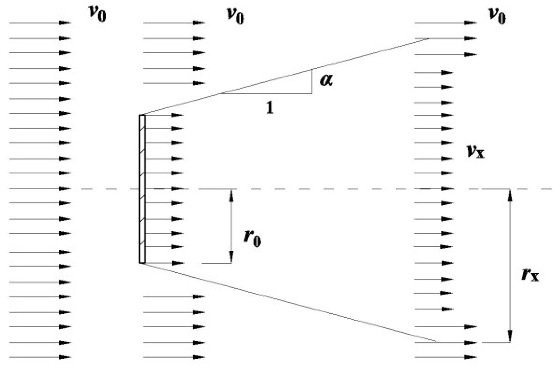
The popular PARK model was initially proposed by Jensen [22] and was further tuned by Katic et al. [23] for the clustered wind turbine research. The improved PARK model has been mostly applied in literature for the wind farm layout optimization study [24]. Figure 2 shows the general properties of the PARK model, which assumes a linear wake propagation behind the upstream wind turbine rotor and notice that the radial wind speed distribution inside the wake is set to be constant.
The wake-affected wind speed at the downstream x distance (horizontally in Figure 2) towards the dominant wind direction is given by:
v x = v 0 [ 1 2 a ( r 0 r 0 + α · x ) 2 ]
where v0 is the undisturbed wind speed, vx is the wake wind speed, and r0 is the downstream rotor radius. According to the actuator disk theory, r0 is calculated based on the wind turbine rotor radius R as:
r 0 = R 1 a 1 2 a  
in which, a is axial induction factor calculated as the percentage of reduction from free-stream wind speed to the rotor-plane wind speed. In Equation (8), α is an entrainment constant, which is determined by the relative surface roughness length (z0) and wind turbine hub height (h) in the empirical mathematical form as [25]:
α = 0.5 ln ( h z 0 )  
In Figure 2, r x is the wake radius which is linearly expressed with the form of:
r x = r 0 + α · x
As mentioned above, Jensen’s wake model is one-dimensional assuming the wake velocity only related to the axial distance towards the dominant wind direction. Further research showed that the wind speed variation in the wake occurs not only in the axial direction (horizontal wind direction in Figure 2), but in the radial wind direction (vertical wind direction in Figure 2) as well. It has been reported that the wind speed profile exhibits an approximately Gaussian axisymmetric shape [26,27]. Hence, a two-dimensional Gaussian wake model was applied for the wind farm layout optimization in this paper and since the model was based on the Jensen’s model, it was named Gaussian-Jensen wake model. The new wake model equation is given by:
u x = A ( 1 σ 2 π e r 2 2 σ 2   ) + B
where u x is the wake wind speed in the Gaussian-Jensen wake model and σ is the standard deviation. According to reference [28], the following equations of equality are formulated:
{ σ = r x 2.58 A ( 2.58 r 2 π e 2.58 2 ) + B = v 0 A + 2 B · r = 2 r · v x
by solving the equation with extra simplification, the arguments of A, B, and σ are obtained as:
{ σ = r x 2.58 B = v 0 A = 2 r x · ( v x v 0 )  
The final wake velocity expression for the Jensen-Gaussian wake model is represented by below formula, and the comparison of wind speed contours between the Jensen’s wake model and the Jensen-Gaussian wake model is shown in Figure 3. As can be seen, Figure 3a shows the Jensen’s model with the constant wind speed in the radial direction while the speed in the radial direction is variable for the Jensen-Gaussian wake model in Figure 3b.
v x = v 0 ( 1 10.32 a 2 π   ( r 0 r 0 + α · x ) 2 · e r 2 2 · ( 2.58 r x ) 2 )
For single wake, the velocity deficit is determined according to the wake interaction patterns with a uniform representation formula:
D e f i c i t = 10.32 a 2 π   ( r 0 r 0 + α · x ) 2 · e r 2 2 · ( 2.58 r x ) 2 A o v e r l a p A r o t o r  
where A o v e r l a p is the overlapping area between the wind turbine wake and the wind turbine rotor. For the partial wake pattern, it was calculated according to the relative wind turbine positions. For the full wake pattern, it was equal to the rotor area A r o t o r .
For the i-th wind turbine influenced by multiple wakes of N wind turbines, its velocity deficit is represented by:
D e f i c i t i = i = 1 N ( 10.32 a 2 π   ( r 0 r 0 + α · x ) 2 · e r 2 2 · ( 2.58 r x ) 2 A o v e r l a p i A o v e r l a p i ) 2 ,   i = 1 ,   2 ,   ,   N
Under simplified wind condition with uniform incoming wind speed v 0 , the final approaching wind speed v i of the wake-affected wind turbine is calculated by:
v i = v 0 ( 1 D e f i c i t i )   ,   i = 1 ,   2 ,   ,   N
Under Weibull distribution wind condition with the wind speed magnitude continuously changing, it has been reported that only the scale parameter of Weibull distribution is affected by the wake effect for wind turbine power output calculation, which gives [29]:
c i = c ( 1 D e f i c i t i ) ,   i = 1 ,   2 ,   ,   N
where c i is the scale parameter of the Weibull distribution for the wake-affected wind turbine.

2.4. Objective Function Fitness Evaluation

In this paper, the optimization objective was to maximize the total wind farm energy production ( P t o t a l ) by taking into account the wake interactions between wind turbine using the wake effect model. Under the simplified wind condition with discrete wind speed and wind direction, the individual wind turbine power output can be directly calculated based on the wake-effected wind speed v i and the wind turbine power curve.
For the realistic wind condition of Weibull distribution with continuous wind speed variation, the means of discretization evaluation method was applied for calculating the wake-affected wind turbine power output as follows.
The discretization method tries to discretize the wind speed into a number of small bins in the same manner as the division of wind direction into several sectors. When the wind turbine produces constant rated power, the produced power P 1 under Weibull distribution equals to P r a t e d 0 2 π p ( θ ) d θ v r a t e d v c u t o u t k ( θ ) c ( θ ) ( v c ( θ ) ) k ( θ ) 1 e ( v c ( θ ) ) k ( θ ) d v . By further operations of discretizing the wind speed region and wind direction region, the discrete mathematical expression is given by:
P 1 = P r a t e d l = 1 N θ ω l 1 { e ( 2 · v r a t e d c ( l 1 ) + c ( l ) ) k ( l 1 ) + k ( l ) 2 e ( 2 · v c u t o u t c ( l 1 ) + c ( l ) ) k ( l 1 ) + k ( l ) 2 }
in which, P r a t e d is the wind turbine rated power, v r a t e d is the rated wind speed, v c u t o u t is the cut out wind speed. The wind direction region [0, 2 π ] is uniformly divided into N θ bins with a constant interval of 2 π / N θ . Each divided wind direction bin has been assigned with a value ( ω ) to indicate the probability of occurrence that wind comes amongst that particular wind direction sector, and the dividing points are marked as θ 0 ,   θ 1 ,   ,   θ N θ 1 with corresponding probability values as ω 0 ,   ω 1 ,   ,   θ N θ 1 . The indices of shape parameter and the scale parameter in each wind direction sector are represented by k and c , respectively.
When the produced power increases with the wind speed, the power P 2 under Weibull distrubution equals to 0 2 π p ( θ ) d θ v c u t i n v r a t e d 0.2963 · v 3 k ( θ ) c ( θ ) ( v c ( θ ) ) k ( θ ) 1 e ( v c ( θ ) ) k ( θ ) d v . By further discretization of the wind speed region and wind direction region, the discrete mathematical expression is represented by:
P 2 = j = 1 N v 0.2963 · ( v j 1 + v j 2 ) 3 l = 1 N θ ω l 1 { e ( 2 · v j 1 c ( l 1 ) + c ( l ) ) k ( l 1 ) + k ( l ) 2 e ( 2 · v j c ( l 1 ) + c ( l ) ) k ( l 1 ) + k ( l ) 2 }
apart from the discretization of wind direction, the region between cut in wind speed and rated wind speed is divided into N v bins with the constant interval of ( v r a t e d v c u t i n ) / N v . The dividing points of the wind speed region were assumed to be v 0 ,   v 1 , ,   v N v 1 , v N v and the forward difference method was applied to calculate the integral of the power output function. Evidently, the calculation accuracy is dependent on the interval density of the discretization. Just like the means of calculating the integral with calculus theory, a smaller discretization interval will increase the accuracy of the wind farm power output calculation by approximation.
The final individual wind turbine power was calculated by summing up the separate power parts as: P i = P 1 + P 2 . On top of the calculated individual wind turbine power output P i , the total wind farm power production ( P t o t a l ) which is calculated as the sum of individual wind turbine power production ( P i ):
P t o t a l = i = 1 N P i
where N is the total number of wind turbines in the wind farm.

3. Results and Discussion

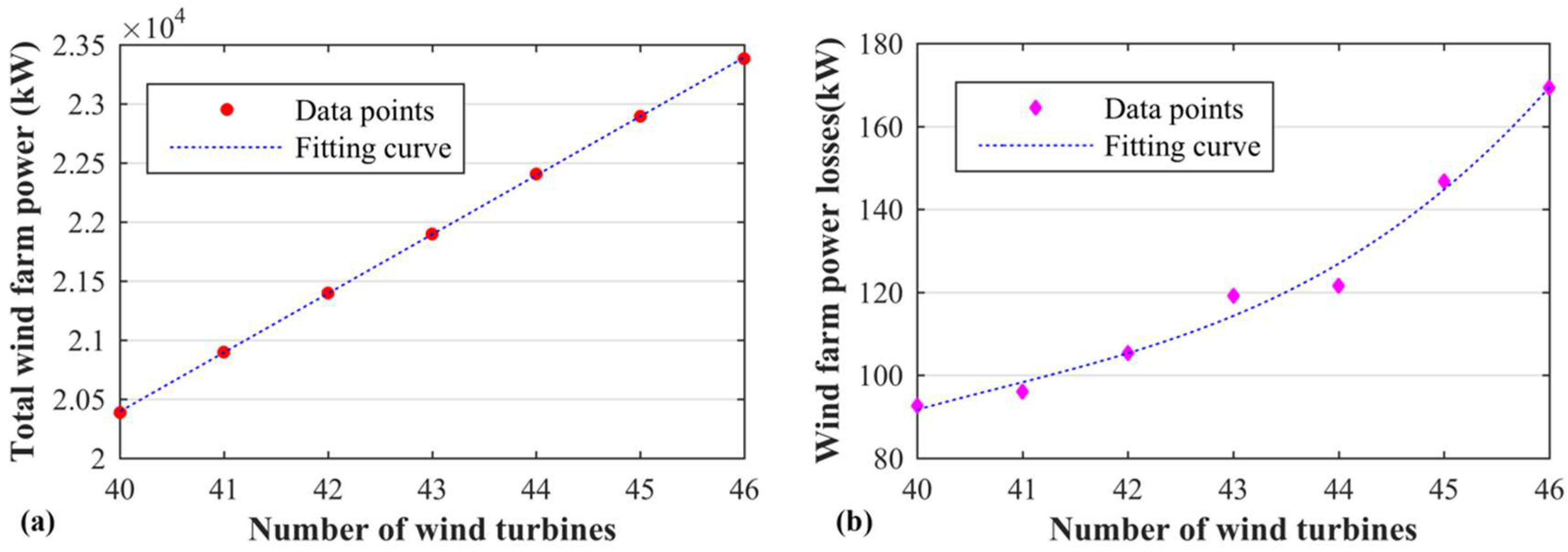
In this paper, the results of wind farm layout optimization under both simplified and realistic wind conditions were presented. Three commonly tested simplified wind conditions in literature were studied, i.e., (i) constant wind speed and constant wind direction; (ii) constant wind speed and variable wind directions; and (iii) variable wind speeds and variable wind directions. Note that due to the lack of detailed wind farm operation information, the continuous number of wind turbine from 40 to 46 was selected for the layout optimization study in this paper to better display the pattern of total wind farm power and power loss variations.

3.1. Constant Wind Speed and Constant Wind Direction

First, the optimization results of a constant 12 m/s wind speed blowing from 0° wind direction were discussed. Figure 4 presents the total wind farm power output and the total wind farm power losses as a function of wind turbine number from 40 to 46. As the number of wind turbines increased, the total power output showed an almost linear increase. However, the power losses increase was relatively small with turbine numbers from 40 to 44. When the number of turbines further increased, large power losses were identified. Figure 5 shows the optimal wind farm layout with 40 wind turbines optimized. The wind direction was 0° which is from the left-hand side to the right-hand side of the figure. As can be seen, most of the wind turbines were distributed along the wind farm boundary. The rest of the wind turbines were spread near to the wind farm boundary, while the center area of the wind farm was free of turbines. Along the wind direction, the distribution of wind turbines showed a staggered pattern in order to avoid the upstream wind turbine wake as much as possible. The minimum distance apart for any two wind turbines was 7 turbine diameters and the average distance of all wind turbines was 37.3 turbine diameters.

3.2. Constant Wind Speed and Variable Wind Directions

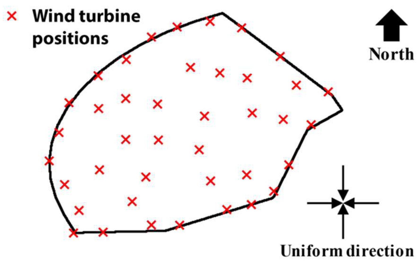
Next, the ideal wind condition of constant wind speed and variable wind directions was studied. The wind condition is shown in Figure 6, and the optimization results of total wind farm power output and power losses as a function of wind turbine number are shown in Figure 7. As can be seen, unlike the above case, both the total wind farm power output and total power losses showed a linear increase with an increasing number of wind turbines. Figure 8 shows the optimal wind farm layout with 40 wind turbines optimized. In general, the wind turbines were uniformly distributed inside the wind farm. The wind farm boundary was fully saturated with distributed wind turbines while the rest of the wind turbines were staggered inside the wind farm area. Due to the characteristics of this ideal wind condition with the equal probability of 360° wind direction, overall the optimal wind turbine distribution seemed much more uniform than the above case. Similar to the above case, minimum distance apart for any two wind turbines was 7 turbine diameters and the average distance of all wind turbines was 36.27 turbine diameters.

3.3. Variable Wind Speeds and Variable Wind Directions

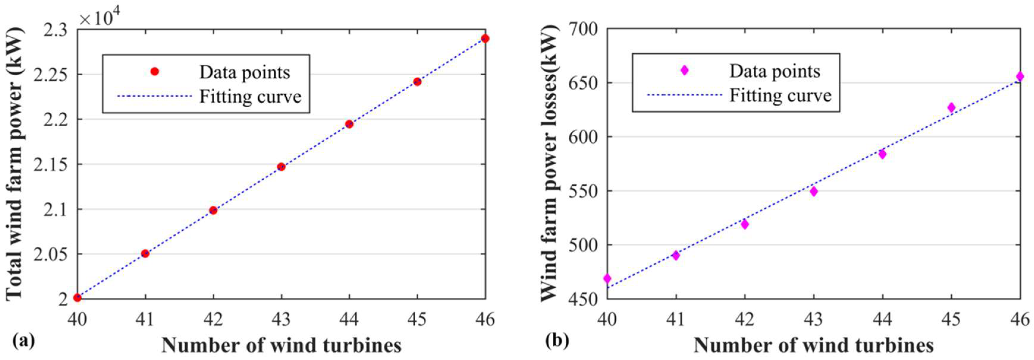
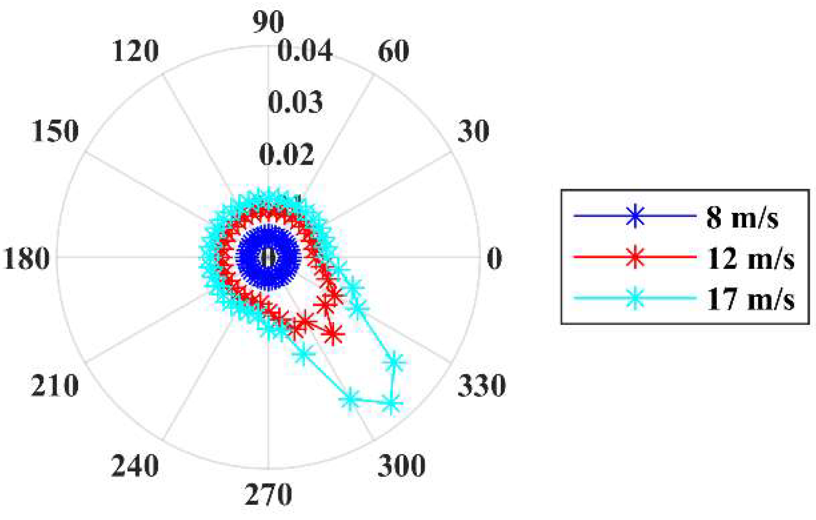
The ideal wind condition of variable wind speeds and variable wind directions was studied, as shown in Figure 9. As can be seen, three different wind speeds i.e., 8 m/s, 12 m/s, and 17 m/s were considered and each wind speed on each wind direction were assigned a particular value indicating its probability of occurrence. Figure 10 shows the optimization results of total wind farm power output and power losses. As the number of wind turbines increased, the total wind farm power output increased linearly and the total power output losses showed a general linearly increasing pattern. Figure 11 shows the optimal wind farm layout with 40 wind turbines optimized. Under this particular wind condition, the wind turbines were distributed all across the wind farm area while they were more aligned to each other compared to the optimal wind farm layouts of the above two cases. The minimum distance apart for any two wind turbines was 7.28 turbine diameters and the average distance of all wind turbines was 36.1 turbine diameters.

3.4. Weibull Distribution Wind Scenario

Finally, a realistic wind condition of Weibull distribution was studied for the wind farm layout optimization. The properties of the Weibull distribution are shown in Table 2. As can be seen, 360° wind direction was equally divided into 24 sections with a 15° interval. In each of the 24 sections, the wind speed variation was represented by the Weibull distribution, where the probability of occurrence of wind blowing amongst that section is indicated by ω. From the table, it is obvious that the predominated wind direction is from 75° to 105°.
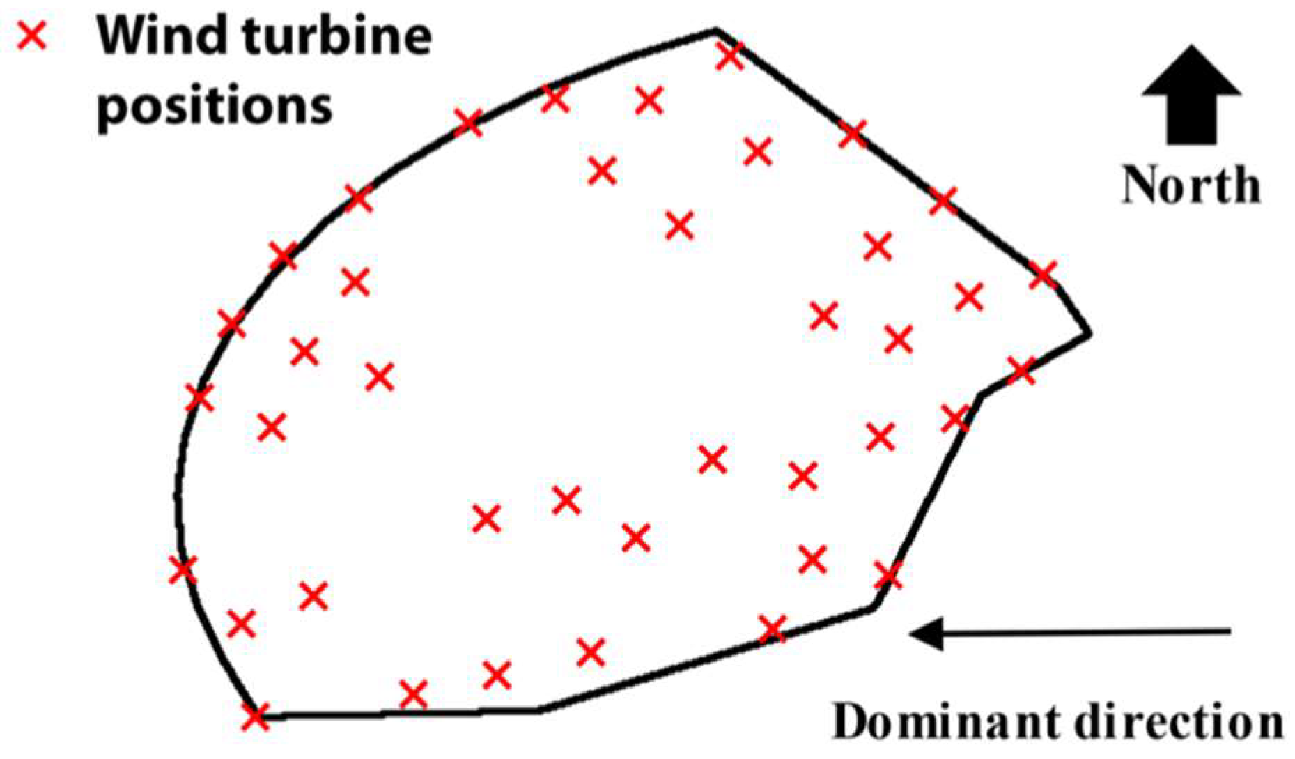
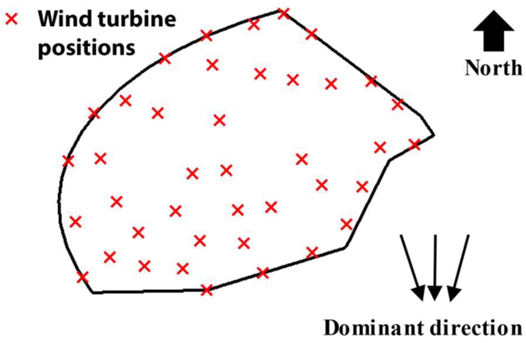
Figure 12 shows the optimization results of total wind farm power output and total power losses under Weibull distribution wind condition. Though the total power output still showed a linear increasing trend with the increasing number of wind turbines, the change of total power losses showed a very different pattern from above cases. In general, the total power losses increased but at some particular numbers of wind turbines (e.g., 41 and 42 wind turbines and 45 and 46 wind turbines), the change of power losses was trivial. The optimal wind farm layout of 40 optimized wind turbines is shown in Figure 13 and the predominant wind direction is from bottom side to the top side. As can be seen, the wind turbines were staggered towards the dominant wind direction to avoid the wake effect as much as possible. Most of the wind turbines were distributed along or near to the wind farm boundary, and part of the inner wind farm area was free of wind turbines in order to enlarge the distance of wind turbines between each other along the dominant wind direction. The minimum distance apart for any two wind turbines was 7 turbine diameters and the average distance of all wind turbines was 35.2 turbine diameters.
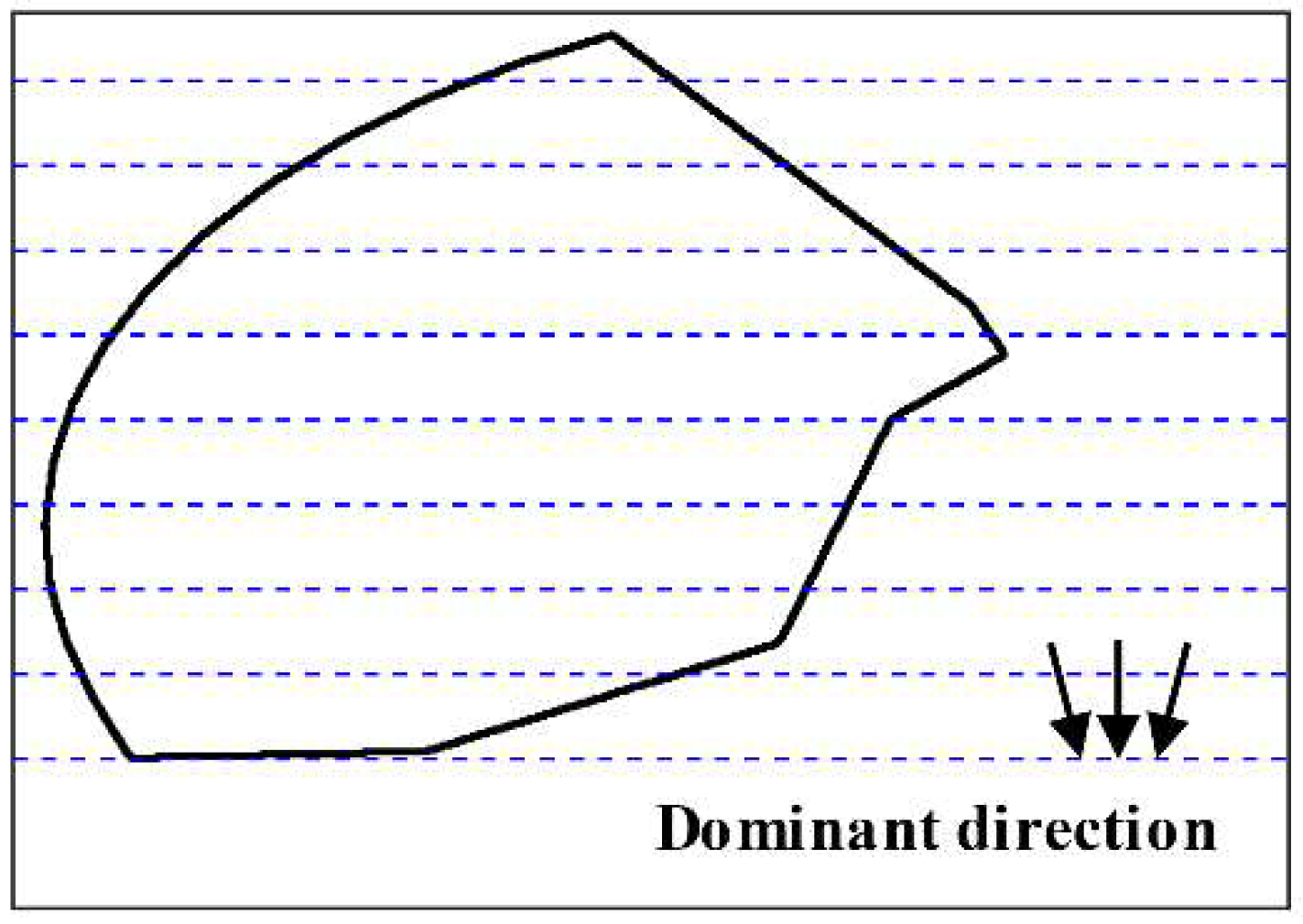
In order to demonstrate the effectiveness of the wind farm layout optimization, the results of optimized wind farm layout and rule of thumb layout (fixed spacing on the cross-wind direction) were compared for the Weibull distribution. Figure 14 shows the schematic of wind farm rule of thumb layout, which had fixed spacing of adjacent wind turbines on the cross-wind direction. The potential wind turbine placements are shown by the dashed lines in Figure 14. Table 3 shows the comparison of total wind farm power output between the rule of thumb layout and optimized layout of wind farm with different number of wind turbines. Evidently, the optimized wind farm layout obtained a larger power production than the rule of thumb layout under this wind characteristic. By comparing to the rule of thumb layout, the power output of the optimized layout improved approximately 17.3%. The properties of optimized wind farm layouts for all tested different wind scenarios are tabulated and compared in Table 4. As can be seen, the minimum distance between wind turbines were the same as the predefined proximity constraint distance (7D) for all scenarios except for the scenario of variable wind speeds and directions, which was slightly larger (7.28D). As the complexity of wind scenario increased, the average distance of wind turbines decreased, indicating a more compact distribution of wind turbines locations. A possible reason for this phenomenon is that a more complex wind scenario demands wind turbines to be placed more “wisely” to mitigate the wake effect, while merely spreading wind turbines over the wind farm area is sufficient to escape the wake effect for a simple wind scenario.

4. Conclusions

In this paper, a real two-dimensional wind farm layout optimization was carried out using the superior unrestricted coordinate method with continuous variation of wind turbine placements. In order to verify the effectiveness of wind farm layout optimization on improving the total output power, different wind conditions including the ideal and realistic wind scenarios were investigated. The ideal wind scenario included constant wind speed and constant wind direction, constant wind speed and variable wind directions, and variable wind speeds and variable wind directions. The realistic wind scenario included a Weibull distribution. A newly developed Jensen-Gaussian wake model, which considers the variation of wake velocity in the radial direction as Gaussian distribution, was employed for the optimization study. The means of handling the irregular wind farm boundary were proposed in conjunction with the discretization method to calculate the wind farm power output under the Weibull distribution. The results showed that as the number of wind turbine increased from 40 to 46, the total wind farm power output showed a linearly increasing pattern. In comparison, the total wind farm power losses variation as a function of the number of wind turbines was dependent on the wind conditions. In general, the total power losses increased with more installed wind turbines. However, for some particular wind conditions, e.g., the Weibull distribution, it showed a different trend with nearly the same power losses when an adjacent number (41 and 42, 45 and 46) of wind turbines were installed. By imposing the boundary constraint on the objective function for optimization, all the optimized wind turbine positions were inside the wind farm boundary. The distribution of wind turbines was dependent on the wind conditions. A common feature of wind turbine positions regardless of wind conditions was that they are distributed along the wind farm boundary as much as possible to alleviate the wake effect.

Author Contributions

Data curation, Y.Z. and J.X.; Writing–review & editing, L.W.

Acknowledgments

This research is funded by the China Postdoctoral Science Foundation (Grant No.: 2018M632244), Natural Science Foundation of Jiangsu Province (Grant No.: BK20180879), High-level Talent Research Foundation of Jiangsu University (Grant No.:18JDG012), Australia Endeavour Scholarships and Fellowships, and Canada Future Energy Systems Program. The financial support from the Jiangsu University of China and Department of Education and Training of Australia are particularly acknowledged. The high performance computational (HPC) resources provided by the Queensland University of Technology (QUT) are also greatly appreciated.

Conflicts of Interest

The authors declare no conflicts of interest.

References

  1. Luo, K.; Yuan, R.; Dong, X.; Wang, J.; Zhang, S. Large-eddy simulation and experimental study on the near wake turbulent flow characteristics of a two-bladed wind turbine. Sci. China Technol. Sci. 2017, 60, 1–28. [Google Scholar] [CrossRef]
  2. Munters, W.; Meyers, J. An optimal control of energy extraction in wind-farm boundary layers. J. Fluid Mech. 2018, 768, 5–50. [Google Scholar]
  3. Mattuella, J.M.L.; Loredo-Souza, A.M.; Oliveira, M.G.K.; Petry, A.P. Wind tunnel experimental analysis of a complex terrain micrositing. Renew. Sustain. Energy Rev. 2016, 54, 110–119. [Google Scholar] [CrossRef]
  4. Wang, L.; Tan, A.C.C.; Cholette, M.E.; Gu, Y. Optimization of Wind Farm Layout with Complex Land Divisions. Renew. Energy 2017, 105, 30–40. [Google Scholar] [CrossRef]
  5. Mosetti, G.; Poloni, C.; Diviacco, D. Optimization of wind turbine positioning in large wind farms by means of a Genetic algorithm. J. Wind Eng. Ind. Aerodyn. 1994, 51, 105–116. [Google Scholar] [CrossRef]
  6. Beyer, H.G.; Rüger, T.; Schäfer, G.; Waldl, H.-P. Optimization of Wind Farm Configurations with Variable Number of Turbines. In Proceedings of the European Union Wind Energy Conference, Göteborg, Sweden, 20–24 May 1996; pp. 1073–1076. [Google Scholar]
  7. Wang, L.; Tan, A.C.C.; Gu, Y. Comparative study on optimizing the wind farm layout using different design methods and cost models. J. Wind Eng. Ind. Aerodyn. 2015, 146, 1–10. [Google Scholar] [CrossRef]
  8. Pérez, B.; Mínguez, R.; Guanche, R. Offshore wind farm layout optimization using mathematical programming techniques. Renew. Energy 2013, 53, 389–399. [Google Scholar] [CrossRef]
  9. Feng, J.; Shen, W.Z. Solving the wind farm layout optimization problem using random search algorithm. Renew. Energy 2015, 78, 182–192. [Google Scholar] [CrossRef]
  10. Chen, Y.; Li, H.; He, B.; Wang, P.; Jin, K. Multi-objective genetic algorithm based innovative wind farm layout optimization method. Energy Convers. Manag. 2015, 105, 1318–1327. [Google Scholar] [CrossRef]
  11. Wang, L.; Cholette, M.E.; Tan, A.C.C.; Gu, Y. A computationally-efficient layout optimization method for real wind farms considering altitude variations. Energy 2017, 132, 147–159. [Google Scholar] [CrossRef]
  12. Kuo, J.Y.J.; Romero, D.A.; Amon, C.H. A mechanistic semi-empirical wake interaction model for wind farm layout optimization. Energy 2015, 93, 2157–2165. [Google Scholar] [CrossRef]
  13. Kuo, J.Y.J.; Romero, D.A.; Beck, J.C.; Amon, C.H. Wind farm layout optimization on complex terrains—Integrating a CFD wake model with mixed-integer programming. Appl. Energy 2016, 178, 404–414. [Google Scholar] [CrossRef]
  14. Parada, L.; Herrera, C.; Flores, P.; Parada, V. Wind farm layout optimization using a Gaussian-based wake model. Renew Energy 2017, 107, 531–541. [Google Scholar] [CrossRef]
  15. Kusiak, A.; Song, Z. Design of wind farm layout for maximum wind energy capture. Renew. Energy 2010, 35, 685–694. [Google Scholar] [CrossRef]
  16. Eroglu, Y.; Seckiner, S.U. Wind farm layout optimization using particle filtering approach. Renew. Energy 2013, 58, 95–107. [Google Scholar] [CrossRef]
  17. Bansal, J.C.; Farswan, P. Wind farm layout using biogeography based optimization. Renew. Energy 2017, 107, 386–402. [Google Scholar] [CrossRef]
  18. Fu, Q.; Yu, D.; Ghorai, J. Probabilistic load flow analysis for power systems with multi-correlated wind sources. In Proceedings of the 2011 IEEE Power and Energy Society General Meeting, Detroit, MI, USA, 24–29 July 2011. [Google Scholar]
  19. Sloughter, J.M.; Gneiting, T.; Raftery, A.E. Probabilistic Wind Speed Forecasting using Ensembles and Bayesian Model Averaging. J. Am. Stat. Assoc. 2010, 105, 25–35. [Google Scholar] [CrossRef]
  20. Salcedo-Sanz, S.; Gallo-Marazuela, D.; Pastor-Sánchez, A.; Carro-Calvo, L.; Portilla-Figueras, A.; Prieto, L. Evolutionary computation approaches for real offshore wind farm layout: A case study in northern Europe. Expert Syst. Appl. 2013, 40, 6292–6297. [Google Scholar] [CrossRef]
  21. Seguro, J.V.; Lambert, T.W. Modern estimation of the parameters of the Weibull wind speed distribution for wind energy analysis. J. Wind Eng. Ind. Aerodyn. 2000, 85, 75–84. [Google Scholar] [CrossRef]
  22. Jensen, N.O. A Note on Wind Generator Interaction; Riso National Laboratory: Roskilde, Denmark, 1983. [Google Scholar]
  23. Katic, I.; Hojstrup, J.; Jensen, N.O. A simple model for cluster efficiency. In Proceedings of the European Wind Energy Conference and Exhibition, Rome, Italy, 7–9 October 1986; pp. 407–410. [Google Scholar]
  24. Wang, L.; Cholette, M.E.; Fu, Y.; Yuan, J.; Zhou, Y.; Tan, A.C.C. Combined optimization of continuous wind turbine placement and variable hub height. J. Wind Eng. Ind. Aerodyn. 2018, 180, 136–147. [Google Scholar] [CrossRef]
  25. Frandsen, S. On the wind speed reduction in the center of large clusters of wind turbines. J. Wind Eng. Ind. Aerodyn. 1992, 39, 251–265. [Google Scholar] [CrossRef]
  26. Chamorro, L.P.; Porté-Agel, F. A wind-tunnel investigation of wind-turbine wakes: Boundary-Layer turbulence effects. Bound.-Lay. Meteorol. 2009, 132, 129–149. [Google Scholar] [CrossRef]
  27. Tian, L.; Zhu, W.; Shen, W.; Zhao, N.; Shen, Z. Development and validation of a new two-dimensional wake model for wind turbine wakes. J. Wind Eng. Ind. Aerodyn. 2015, 137, 90–99. [Google Scholar] [CrossRef] [Green Version]
  28. Gao, X.; Yang, H.; Lu, L. Optimization of wind turbine layout position in a wind farm using a newly-developed two-dimensional wake model. Appl. Energy 2016, 174, 192–200. [Google Scholar] [CrossRef]
  29. Lackner, M.A.; Elkinton, C.N.C. An Analytical Framework for Offshore Wind Farm Layout Optimization. Wind Eng. 2007, 31, 17–31. [Google Scholar] [CrossRef]
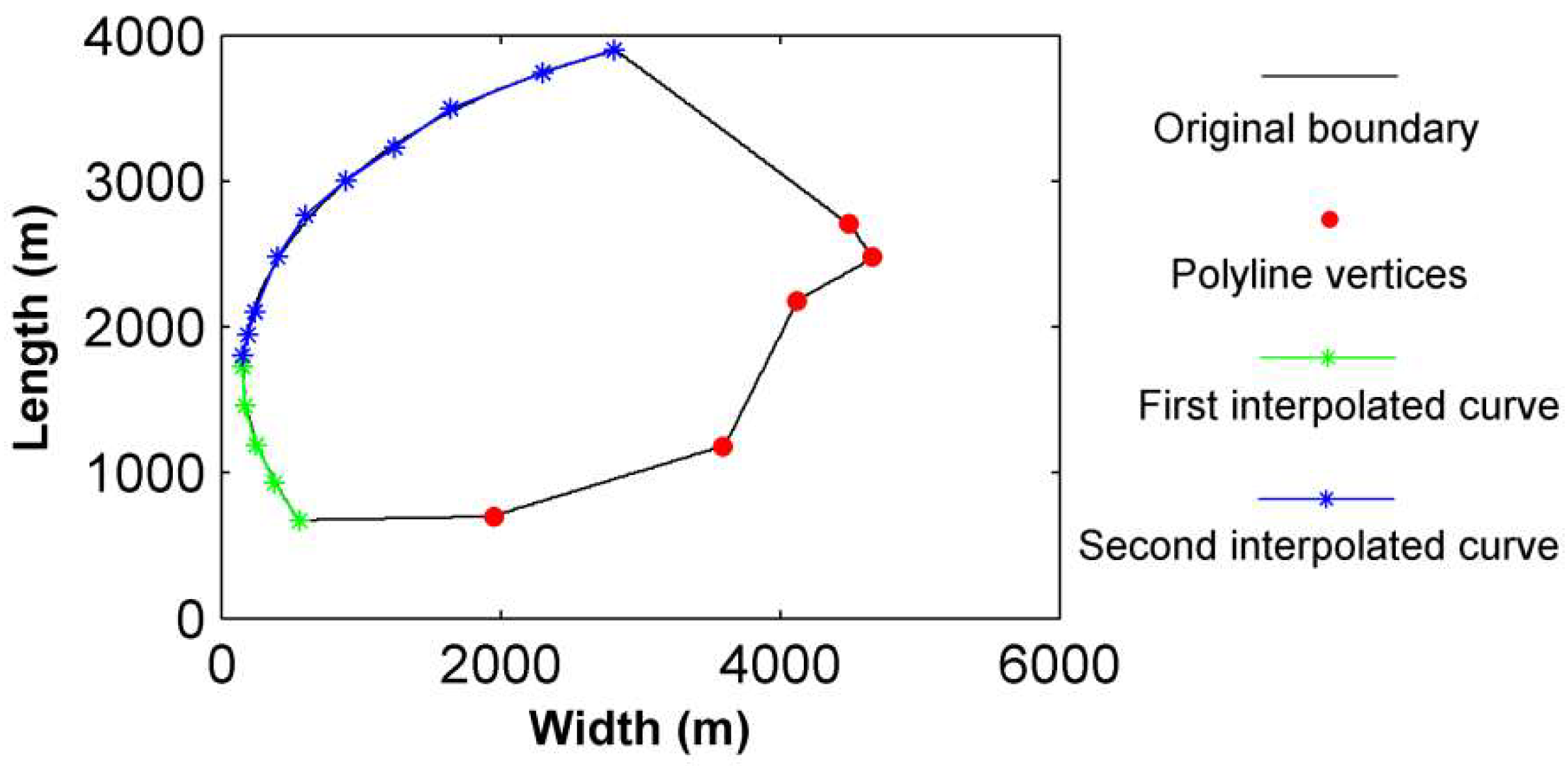
Figure 1. Diagram of the irregular wind farm boundary representation.
Applsci 08 02660 g001
Figure 2. Diagram of one-dimensional Jensen’s wake model.
Applsci 08 02660 g002
Figure 3. Comparison of the normalized wind speed contours in the wake calculated by: (a) one-dimensional Jensen wake model and (b) two-dimensional Jensen-Gaussian wake model.
Applsci 08 02660 g003
Figure 4. Results of wind farm layout optimization with different number of wind turbines under constant wind speed and constant wind direction: (a) wind farm power production and (b) wind farm power losses.
Applsci 08 02660 g004
Figure 5. Optimal wind farm layout with 40 wind turbines under constant wind speed and constant wind direction.
Applsci 08 02660 g005
Figure 6. Probability of constant wind speed and variable wind directions.
Applsci 08 02660 g006
Figure 7. Results of wind farm layout optimization with different number of wind turbines under constant wind speed and variable wind directions: (a) wind farm power production and (b) wind farm power losses.
Applsci 08 02660 g007
Figure 8. Optimal wind farm layout with 40 wind turbines under constant wind speed and variable wind directions.
Applsci 08 02660 g008
Figure 9. Probability of variable wind speeds and variable wind directions.
Applsci 08 02660 g009
Figure 10. Results of wind farm layout optimization with different number of wind turbines under variable wind speeds and variable wind directions: (a) wind farm power production and (b) wind farm power losses.
Applsci 08 02660 g010
Figure 11. Optimal wind farm layout with 40 wind turbines under variable wind speeds and variable wind directions.
Applsci 08 02660 g011
Figure 12. Results of wind farm layout optimization with different number of wind turbines under Weibull distribution wind condition: (a) wind farm power production and (b) wind farm power losses.
Applsci 08 02660 g012
Figure 13. Optimal wind farm layout with 40 wind turbines under Weibull distribution wind condition.
Applsci 08 02660 g013
Figure 14. Rule of thumb layout of wind farm with fixed spacing of potential wind turbine locations on the cross-wind direction.
Applsci 08 02660 g014
Table 1. Properties of the wind turbine model for the real offshore wind farm.
ParametersValues
Rated power1000 kW
Rotor diameter54 m
Hub height60 m
Cut-in wind speed3 m/s
Rated wind speed15 m/s
Cut-out wind speed25 m/s
Cubic power curveP = 0.2963 v i 3 kW
Table 2. Detail of the Weibull distribution wind condition.
DirectionkcωDirectionkcω
0°~15°290180°~195°290.01
15°~30°290.01195°~210°290.01
30°~45°290.01210°~225°290.01
45°~60°290.01225°~240°290.01
60°~75°290.01240°~255°290.01
75°~90°290.2255°~270°290.01
90°~105°290.6270°~285°290.01
105°~120°290.01285°~300°290.01
120°~135°290.01300°~315°290.01
135°~150°290.01315°~330°290.01
150°~165°290.01330°~345°290.01
165°~180°290.01345°~0°290.01
Table 3. Comparison of total wind farm power output (in kW) with different number of wind turbines for rule of thumb layout and optimized wind farm layout.
Number40414243444546
Layout
Rule of thumb8373858487858982919993959598
Optimized982110,05610,30310,54010,78211,01711,263
Table 4. Comparison of optimized wind farm layouts in terms of minimum and average distances between wind turbines (in the unit of turbine diameter, D) for different wind scenarios studied.
Layout PropertiesMinimum Distance of Wind TurbinesAverage Distance of Wind Turbines
Wind Scenario
Constant speed and direction7D37.3D
Constant speed and variable directions736.27D
Variable speeds and directions7.28D36.1D
Weibull distribution7D35.2D