Article

Estimation of High-Resolution Daily Ground-Level PM2.5 Concentration in Beijing 2013–2017 Using 1 km MAIAC AOT Data

1
School of Automation Engineering, University of Electronic Science and Technology of China, Chengdu 611731, China
2
College of Resources and Environment, University of Chinese Academy of Sciences, Beijing 100049, China
3
Lamont-Doherty Earth Observatory of Columbia University, Palisades, NY 10964, USA
4
Center for International Earth Science Information Network, Earth Institute, Columbia University, Palisades, NY 10964, USA
*
Author to whom correspondence should be addressed.
Appl. Sci. 2018, 8(12), 2624; https://doi.org/10.3390/app8122624
Submission received: 22 November 2018 / Revised: 9 December 2018 / Accepted: 11 December 2018 / Published: 14 December 2018
(This article belongs to the Special Issue Monitoring and Modeling: Air Quality Evaluation Studies)

Abstract

:

Featured Application

This work has several applications: (a) to reveal spatiotemporal variations of PM2.5 across urban landscapes; (b) to assess the long-term impacts of PM2.5 on human health; (c) to support government policy decision-making; and (d) to provide valuable information to the public.

Abstract

High-spatiotemporal-resolution PM2.5 data are critical to assessing the impacts of prolonged exposure to PM2.5 on human health, especially for urban areas. Satellite-derived aerosol optical thickness (AOT) is highly correlated to ground-level PM2.5, providing an effective way to reveal spatiotemporal variations of PM2.5 across urban landscapes. In this paper, Multi-Angle Implementation of Atmospheric Correction (MAIAC) AOT and ground-based PM2.5 measurements were fused to estimate daily ground-level PM2.5 concentrations in Beijing for 2013–2017 at 1 km resolution through a linear mixed effect model (LMEM). The results showed a good agreement between the estimated and measured PM2.5 and effectively revealed the characteristics of its spatiotemporal variations across Beijing: (1) the PM2.5 level is higher in the central and southern areas, while it is lower in the northern and northwestern areas; (2) the PM2.5 level is higher in autumn and winter, while it is lower in spring and summer. Moreover, annual PM2.5 concentrations decreased by 24.03% for the whole of Beijing and 31.46% for the downtown area from 2013 to 2017. The PM2.5 data products we generated can be used to assess the long-term impacts of PM2.5 on human health and support relevant government policy decision-making, and the methodology can be applied to other heavily polluted urban areas.

Graphical Abstract

1. Introduction

PM2.5 refers to atmospheric particulate matter (PM) with a diameter of less than 2.5 micrometers, which remains suspended for a longer time in the air. Numerous studies have demonstrated that exposure to PM2.5 is associated with adverse health effects including respiratory and cardiovascular diseases [1,2,3]. In urban areas, PM2.5 concentrations vary sharply over short distances caused by uneven distribution of emission sources, diffusion, and physicochemical transformations. While traditional ground-based monitoring measures PM2.5 concentrations with high temporal resolution (e.g., daily and hourly), the monitoring sites are generally distributed sparsely and unevenly, lacking the spatial resolution necessary to analyze the fine-scale spatial variability of pollution; this variability is important for health impact assessment and is needed to characterize the heterogeneity of human exposure to PM2.5, analyze its adverse health effects, and effectively prevent and control air pollution [4].
Aerosol optical thickness (AOT), defined as the integrated extinction coefficient over a vertical column of atmosphere at an observation location, is a measure of the extinction of the solar beam by aerosol particles in the atmosphere. Satellite-derived AOT can be used to monitor urban air quality through adding synoptic and spatial distribution information to ground-based air quality data and modeling [5]. Different approaches have been employed to estimate surface PM2.5 concentrations from AOT, with many efforts on developing linear regression models to effectively relate PM2.5 and AOT [6,7]. For example, meteorological data have been incorporated in a multiple regression analysis and improved the PM2.5–AOT correlation [8]; considering that spatial variation of pollution may introduce significant biases, a geographically weighted regression model (GWR) was developed to accommodate such spatial variations [9,10,11]; and local scaling factors obtained from a global chemical transport model (GEOS-Chem) were combined with AOT to estimate ground-level PM2.5 [12]. Taking time-varying parameters into account, a statistical model was developed to calibrate 10 km MODIS AOT and predict daily PM2.5 concentrations [13], and this model was further improved through adding meteorological data, land use, and pollution sources [14,15,16,17,18,19,20,21,22,23], and applied in the Beijing area to estimate PM2.5 spatial variations using Moderate Resolution Imaging Spectroradiometer (MODIS) AOT data products at 3 km resolution [24,25].
In this study, considering the attention paid to the linear mixed effect model (LMEM) developed by Lee et al. [13] and its demonstrated effectiveness, we assessed the performance of the LMEM in heavily polluted urban areas. Specifically, the results of LMEM fitting with AOT at 1 km and 3 km resolutions and different PM2.5 datasets were compared, the spatiotemporal trends of PM2.5 pollution in Beijing from 2013 to 2017 were analyzed, and the effectiveness of government policies regarding air pollution mitigation in recent years was evaluated.

2. Materials and Methods

2.1. Study Area

Beijing, the capital of China, is located in northeastern China at the northern tip of the North China Plain, near the meeting point of the Xishan and Yanshan mountain ranges (Figure 1). In recent years, it has been experiencing heavy air pollution because of the enormous economic boom, the increase in the number of motorized vehicles, population growth, the surrounding topography, and seasonal weather conditions. By 2015, the population living in Beijing metropolitan areas was over 21 million, with about 2.1 million children and 2.2 million elders. This makes Beijing a study area quite suitable for air pollution research.

2.2. Ground-Level PM2.5 Data Sets

Ground-level PM2.5 data sets were used for model parameterizing and accuracy assessment in this study. PM2.5 data are collected hourly in Beijing from totally 35 monitoring sites located in the metropolitan area (Figure 1, Table S1). The data sets are managed by the Beijing Municipal Environmental Monitoring Center (BMEMC). In this study, the hourly ground-level PM2.5 concentrations were averaged to get two PM2.5 datasets at each monitoring site for five years from 1 January 2013 through 31 December 2017: (1) the PM2.5 24 h average between 00:00 a.m. and 23:00 p.m. and (2) the PM2.5 period average between 10:00 a.m. and 2:00 p.m.

2.3. AOT Data Sets

The major AOT data sets used in this study were the MAIAC AOT data sets, which are produced using a generic algorithm specifically developed for MODIS, performing aerosol retrievals and atmospheric correction over both vegetated surfaces and bright deserts at 1 km spatial resolution based on time series analysis and image processing [26,27]. The MAIAC algorithm also derives column water vapor (CWV), the surface reflectance (SR) bidirectional reflectance distribution function (BRDF), and spectral regression coefficients (SRC). MAIAC collects 5 (over poles) to 16 (over equator) days of MODIS observations depending on locations on the Earth using a sliding window approach. These MODIS observations are then gridded to 1 km spatial resolution with specific projection coordinate systems. When the land surface conditions remain stable during a data collection period, the surface BRDF is retrieved using the regional background aerosol model. The 2.1 μ m MODIS band is used to retrieve AOT and surface reflectance over dark and moderately bright surfaces. Four or more low AOT days are used to calculate the SRC correlating surface reflectance in the blue and shortwave infrared bands. Once the SRC is obtained, the AOT is retrieved with the last MODIS observation. AOT retrieval is conducted with the regional background aerosol model in clear conditions, but with surface BRDF in hazy conditions. Aerosol Robotic Network (AERONET) [28] validation shows that the MAIAC and the MODIS Level-2 atmospheric aerosol product (MOD04 ) algorithms have similar accuracy over dark and vegetated surfaces and that MAIAC AOT generally improves in accuracy over brighter surfaces due to SRC retrieval and explicit BRDF factor characterization, as demonstrated for several U.S. West Coast AERONET sites [26].
MAIAC AOT data sets derived from Terra (at ~10:30 a.m. local time) and Aqua (at ~1:30 p.m. local time) were merged to improve its spatial coverage in urban areas [14]. For a given day, due to meteorological condition changes and other factors, the two MAIAC AOT measurements might vary slightly. When merging the AOT data for a given area and a given day, there are two possible cases regarding the availability of AOT data: (1) both MAIAC-Aqua AOT and MAIAC-Terra AOT are available, or (2) only one of the two MAIAC AOTs is available. In the second case, the missing AOT values were estimated through a regression model. As a result, the daily AOT average represents the average between 10:00 a.m. and 2:00 p.m. for each day. As the ratio of morning AOT and afternoon AOT varies by season, we reorganized all the AOT data sets into two seasons for each year: warm season (15 April–14 October) and cold season (15 October–14 April). For the missing AOT estimation, the R2 values of the regression model in warm and cold seasons were 0.88 and 0.87 respectively, indicating a good regression-based AOT interpolation.
For comparison purposes, MODIS Collection 6 Level 2 aerosol data products with 3 km spatial resolution (MOD-3K AOT) for 2014 were also collected. The algorithm for generating MOD-3K AOT is similar to the algorithm used in the previous 10 km AOT product, but the MOD-3K AOT algorithm averages 6 × 6 pixels in a single retrieval box rather than 20 × 20 pixels after cloud screening and other surface mask processes [29]. The MOD-3K AOT products have been validated by ground-based measurements from six AERONET sites in China, and its spatiotemporal variations show good agreement with the AERONET AOT, with R2 values of 0.80–0.97 at the six sites [30].

2.4. Data Preprocessing

To establish the PM2.5–AOT relationship model (parameterization), the ground-based PM2.5 measurements and satellite-derived MAIAC AOT values must be collected at the closest spatial location and time. For each monitoring site (PM2.5), the 1 km pixel of MAIAC AOT where the monitoring site locates was selected and its AOT value was extracted to form a PM2.5–AOT data pair. PM2.5–AOT data pairs with either PM2.5 values less than 3.0 μg/m3 or missing PM2.5/AOT measurements were omitted. In addition, the days with less than two PM2.5–AOT data pairs available were excluded as a regression slope cannot be estimated from only a single data pair. MAIAC AOT pixels of water areas were removed through flagging because the high moisture content around water areas tends to be misidentified as PM2.5 by estimation models.

2.5. LMEM Model Fitting and Validation

Lee et al. [13] developed the LMEM algorithm to estimate PM2.5 from MODIS MOD04 AOT at 10 km resolution; it takes into account the day-to-day variability of the PM2.5–AOT relationship based on mixing height, relative humidity, PM2.5 composition, and PM2.5 vertical profile with the assumption that the PM2.5–AOT relationship varies largely day to day but minimally spatially on a given day at the study area. The LMEM calculates day-specific random intercepts and slopes for the PM2.5–AOT relationship and incorporates both fixed-effects terms and random-effects terms. The LMEM equation is
P M i j = ( α + μ j ) + ( β + υ j ) × AOT ij + s i + ε ij
where P M i j is the daily average PM 2.5 concentration at site i on day j; A O T i j is the daily average AOT value corresponding to site i on day j; α and μ j are the fixed and random intercepts on day j, respectively; β and υ j are the fixed and random slopes on day j, respectively; s i is the random intercept of site i; and ε ij is the error term at site i on day j. In this model, the fixed parameter β for AOT represents the average PM2.5–AOT relationship for the entire space and time in the specific urban area, while the random parameter υ j represents daily variation of the PM2.5–AOT relationship.
We trained (fitting and validating) the LMEM using a large number of PM2.5–AOT sample data pairs for PM2.5 estimation from 2013 to 2017. As an AOT pixel value represents the average aerosol level in a given 1 km × 1 km area while a ground-based PM2.5 measurement only represents the aerosol level at a point, theoretically, there may be systematic bias between AOT-derived PM2.5 and ground-measured PM2.5. The site bias may also vary by surface cover type, topography, distance to pollution source, and other anthropogenic and natural environmental conditions. It should be noted that site random effect ( s i ) was not considered when estimating PM2.5 concentrations for our study period because AOT values are unbiased representative of the corresponding grid cells; in other words, PM2.5 values derived from AOT reflect the overall PM2.5 levels in the grid cell, but the unadjusted predicted PM2.5 levels with site effects maybe be more representative of the average population exposures to PM2.5 [13].
After the model training, the PM2.5 estimates over our study area for the whole time period were generated using LMEM and 1 km MAIAC AOT. Further, the model performance using 1 km AOT data and 3 km AOT data was compared using the 1 km MAIAC AOT and 3 km MOD-3K AOT data sets for 2014 as inputs. In addition, as the PM2.5 24 h average and the PM2.5 period average may differ, we also established different LMEM models and compared the model performance with these two PM2.5 data sets.
Tenfold cross-validation (CV) was applied to test the potential model overfitting through randomly splitting the entire samples (PM2.5–AOT pairs) into 10 subsets with each subset containing approximately 10% of the whole sample dataset. One sample subset was used for model testing, while the remaining nine sample subsets were used for model fitting. This procedure was repeated 10 times until every subset was tested. The site-specific (each site) R2 between estimated PM2.5 and ground-based PM2.5 measurements, mean prediction error (MPE), and root-mean-squared prediction error (RMSPE) were calculated for model fitting and cross validation results:
M P E = i = 1 n ( y i y i ) / n
RMSPE = i = 1 n ( y i y i ) 2 / n
where y i and y i are the estimated PM2.5 and the measured PM2.5 of the ith sample, respectively, and n is the total number of PM2.5–AOT sample pairs.

3. Results

3.1. Data Descriptive Statistics

In this study, there were 33,785 PM2.5–AOT sample pairs in total for the 35 monitoring sites and 1301 days (239 days for 2013, 261 days for 2014, 268 days for 2015, 269 days for 2016, and 264 days for 2017), which were used for model fitting and model validation. The number of PM2.5–AOT sample pairs varies from 666 to 1015 by site. The data statistics demonstrate that the overall mean of the PM2.5 24 h average is 72.15 μg/m3, varying from 44.95 μg/m3 (SD = 46.89 μg/m3) to 105.02 μg/m3 (SD = 87.29 μg/m3) by site (Table S2), and the overall mean of the PM2.5 period average between 10:00 a.m. and 2:00 p.m. is 65.82 μg/m3, varying from 39.39 μg/m3 (SD = 47.49 μg/m3) to 92.33 μg/m3 (SD = 87.36 μg/m3) by site (Table S3). The overall mean MAIAC AOT is 0.49, varying from 0.30 (SD = 0.32) to 0.61 (SD = 0.66) by site (Table S4). As shown in Figure 1, the study area is surrounded by mountains in the west, north, and northeast, while it is quite flat in the south and southeast. PM2.5 levels have an increasing gradient trend from north to south, and the spatial distribution of the MAIAC AOT average and PM2.5 levels for the whole study time period has a similar spatial pattern. The consistency of the spatial trends between the MAIACT AOT average and PM2.5 levels indicates the correlation of AOT and PM2.5.

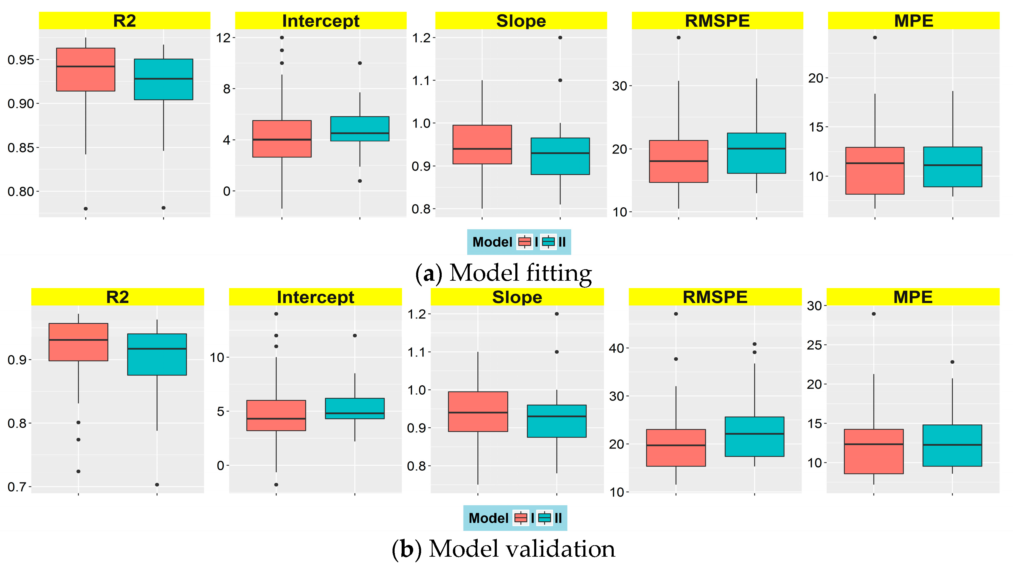
3.2. Results of Model Fitting and Validation

We fitted the LMEM PM2.5 estimation model for each year using the two different daily PM2.5 data sets—the PM2.5 24 h average (Model-I) and the PM2.5 period average (Model-II)—and 1 km MAIAC AOT. Figure 2a shows the model fitting performance statistics (R2, Intercept, Slope, RMSPE, and MPE) at each site, with site-specific R2 ranging from 0.72 to 0.97, Slope from 0.75 to 1.1, RMSPE from 11.50 μg/m3 to 47.08 μg/m3, and MPE from 7.17 μg/m3 to 28.93 μg/m3 for Model-I; and R2 ranging from 0.70 to 0.96, Slope from 0.78 to 1.2, RMSPE from 15.28 μg/m3 to 40.81 μg/m3, and MPE from 8.56 μg/m3 to 22.80 μg/m3 for Model-II. The median values of R2 and Slope for Model-I are higher than those for Model-II, and its Model-I’s RMSPE values are lower.
The model fitting performance for each year can be seen in Figure 3a and Table 1: the year-specific R2 of Model-I ranges from 0.90 to 0.94 and is 0.90 for the whole study period, while the year-specific R2 of Model-II ranges from 0.91 to 0.93 and is 0.92 for the whole study period. Therefore, both Model-I and Model-II have high R2 values (more than 0.90), demonstrating that both the PM2.5 24 h average and the PM2.5 period average between 10:00 a.m. and 2:00 p.m. can be used to fit the estimation model with high estimation performance. However, the other model fitting statistics indicate that Model-I performs slightly better than Model-II. In addition, model cross validation performance statistics are shown in Figure 2b for each site, and in Figure 3b and Table 1 for each year: Figure 2b shows that the site-specific R2 for both Model-I and Model-II decreases, while RMSPE and MPE increase from model fitting to model validation with small differences. The yearly model cross validation results shown in Figure 3b and Table 1 indicate that the year-specific R2 of Model-I ranges from 0.87 to 0.93 and is 0.90 for the whole study period, while the year-specific R2 of Model-II ranges from 0.89 to 0.92 and is 0.90 for the whole study period. Overall, although both Model-I and Model-II have good estimation performance with high R2 values, Model-I is relatively better as it has lower RMSPE and MPE values.
We fitted the model for each year and estimated the daily PM2.5 concentrations for the period from 2013 through 2017. The annual mean PM2.5 concentrations and five-year (2013–2017) mean PM2.5 concentrations were generated for different seasons (warm and cold) and for specific urban areas (the whole urban area and the central city area) using estimated daily PM2.5 concentrations in order to reveal the spatiotemporal variations of PM2.5 levels.
To better assess the model performance, we also experimented on the 3 km MOD-3K AOT for the year 2014, and the results are shown in Table 2. The model performance results for the 3 km AOT are given in Table 2 and in Figure 4, Figure 5 and Figure 6. Based on comparing the R2, RMSPE, and MPE, slightly better performance of Model-I than Model-II is also observed at 3 km resolution. As a result, we employed Model-I to estimate the daily PM2.5 concentrations for the study area during the period 2013–2017.

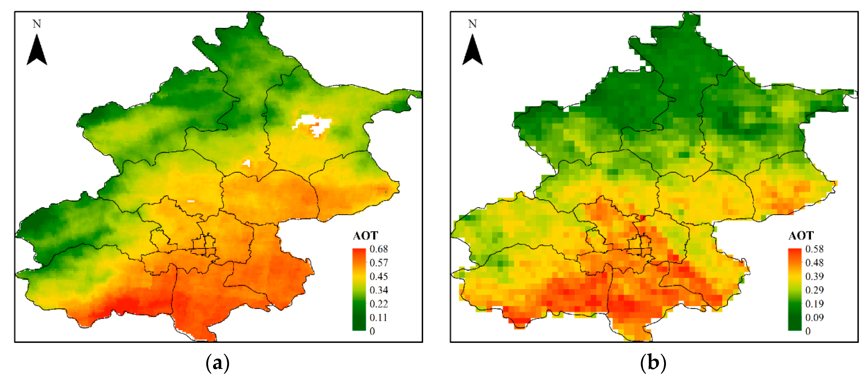
3.3. Comparing between Estimated and Measured PM2.5 Concentrations

The differences between the Model-I estimated and measured PM2.5 concentrations are shown in Figure 7. It can be observed that the PM2.5 concentrations are slightly overestimated in lightly polluted areas, while they are slightly underestimated in heavily polluted areas. However, the differences are within ±10.90 μg/m3, and a relative difference of 15.67% for 85% of all the monitoring sites indicates a good agreement between them.

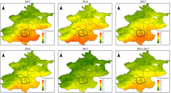
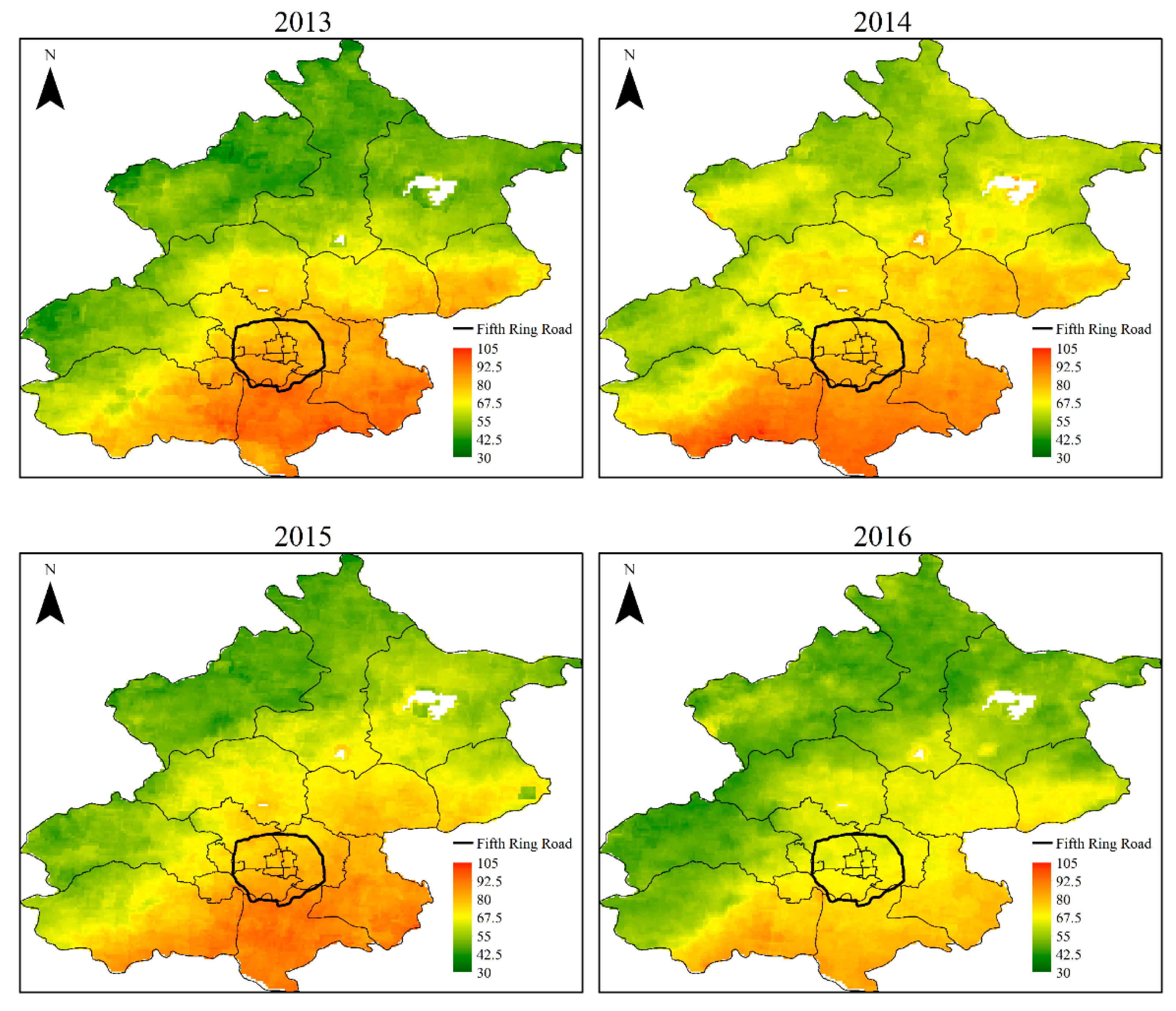
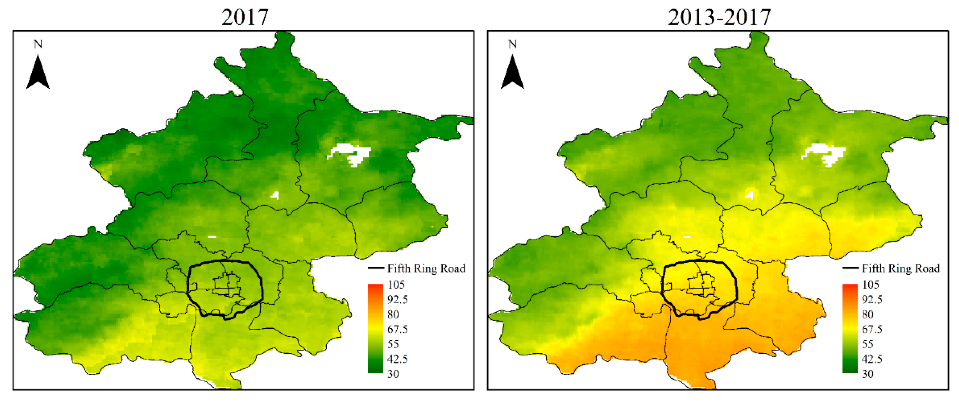
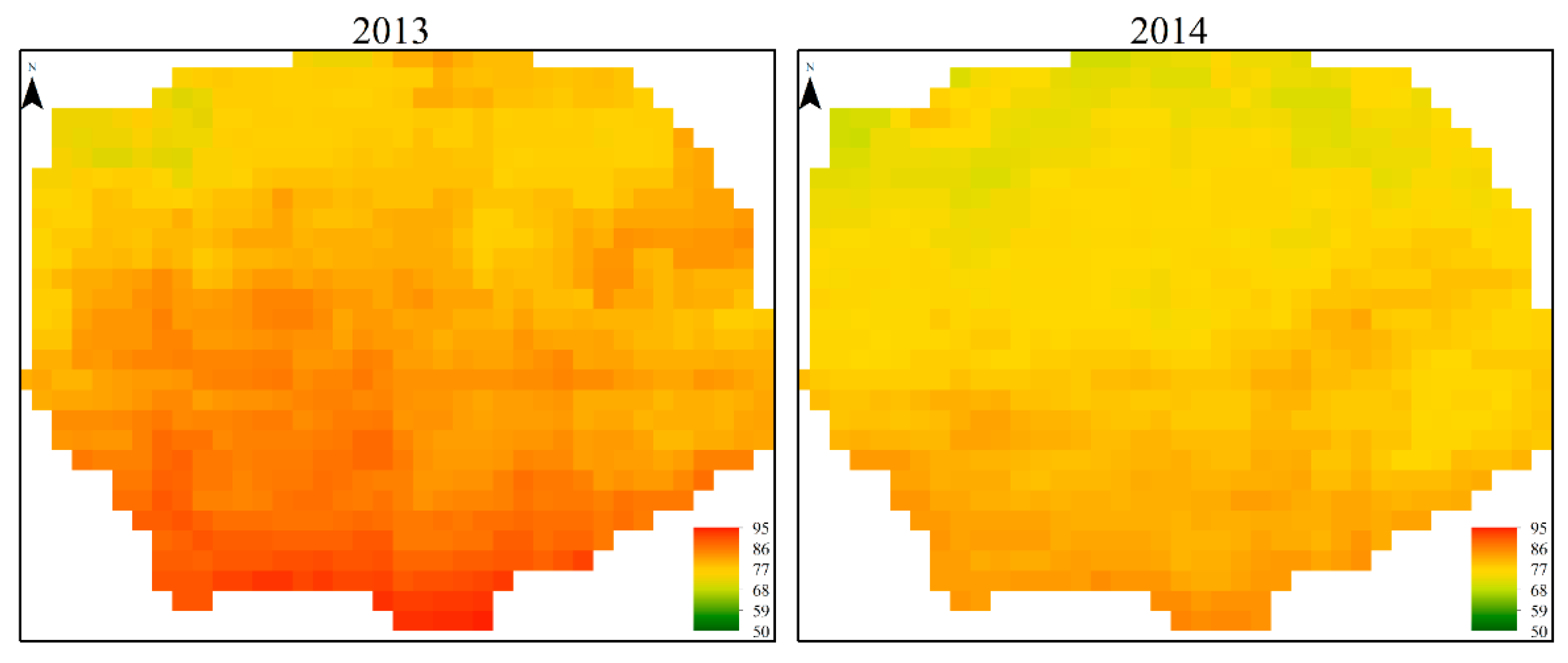
3.4. Spatiotemporal Trends of PM2.5 Concentrations

Using the above Model-I, we can create daily, weekly, monthly, seasonal, and annual mean PM2.5 maps which can be applied in health effect analysis, air pollution management, and mitigation policy decision-making support. Figure 8 illustrates the annual mean maps of MAIAC AOT-derived PM2.5 estimations at 1 km spatial resolution in the study area from 2013 to 2017. The annual mean estimated PM2.5 concentrations are 63.93, 69.09, 65.28, 59.17, and 48.56 μg/m3 from 2013 to 2017, respectively. These maps revealed the significantly similar spatial patterns of PM2.5 concentrations across the Beijing metropolitan area during the study period: high PM2.5 levels are located in the southern parts which are closer to the major pollution sources from the Hebei Province and in the upwind direction of Hebei, while low PM2.5 levels appear in rural and mountainous areas in the northern parts. This corresponds well with the spatial patterns demonstrated by the ground-based monitoring shown in Figure 1c.
The area within the Fifth Ring Road is the downtown area of Beijing with the highest population density and heaviest traffic flow. Figure 9 illustrates the annual mean PM2.5 estimates in the downtown area from 2013 to 2017, showing that PM2.5 levels are apparently reduced, especially in 2017 with much lower PM2.5 levels. The annual mean PM2.5 estimates in this downtown area are 81.56, 77.50, 80.04, 67.38, and 55.90 μg/m3 from 2013 to 2017, respectively. Within the downtown area, PM2.5 levels in the northern part are much lower than those in the southern part.
The seasonal mean PM2.5 estimates (Figure 10) for the entire Beijing metropolitan area are 66.10, 45.33, 60.17, and 75.59 μg/m3 for spring (March, April, and May), summer (June, July, and August), autumn (September, October, and November), and winter (December, January, and February), respectively, indicating that PM2.5 levels exhibit distinct seasonal variations, with the highest PM2.5 levels in winter and the lowest in summer. Such seasonal variations can be attributed to the mixed contributions from meteorological conditions (planetary boundary layer height (PBLH), relative humidity, seasonal wind, etc.) and local pollution sources such as coal combustion for domestic heating in winter. Moreover, the seasonal mean PM2.5 has similar spatial patterns with the annual mean PM2.5; that is, higher concentrations occur in the southern part and lower concentrations occur in the northern part.

4. Discussion

In this study, we investigated daily ground-level PM2.5 estimates at 1 km spatial resolution in the Beijing metropolitan area using the LMEM by incorporating the MAIAC AOT data and ground-based PM2.5 measurements. The results show that both model fitting and cross validation can generate higher R2 values for monitoring sites. We also analyzed the model performance for each year in the five-year study period, indicating that both Model-I and Model-II give higher model fitting R2 values and cross validation R2 values relative to a linear regression model based on the same data inputs (Figure S1), and can be hugely improved when considering that daily variations of PM2.5–AOT relationship are correlated to mixing height, relative humidity, PM2.5 composition, and PM2.5 vertical profile. Both Model-I and Model-II have higher R2 values, indicating that the PM2.5 24 h average and the PM2.5 period average between 10:00 a.m. and 2:00 p.m. can be used to fit LMEM models with high confidence. Overall, Model-I has slightly better performance as demonstrated by its lower RMSPE and MPE values and similar R2 values to Model-II.
AOT represents the amount of aerosols in the vertical column of atmosphere from the ground to satellite sensors (not only limited to the vertical column segment close to the monitoring sites). The PM2.5 24 h average captures more of the aerosols which have subsided down to ground level at monitoring sites than does the PM2.5 period average between 10:00 a.m. and 2:00 p.m. This might explain why the LMEM model fitted with the PM2.5 24 h average performs a little better than the LMEM model fitted with the PM2.5 period average.
The LMEM in our study generated higher model fitting R2 values of 0.90–0.94 and cross validation R2 values of 0.87–0.93 than those in previous studies. For example, the GWR model applied to the whole of China with an overall cross validation R2 value of 0.64 [31] and to the Pearl River Delta region with an R2 value of 0.74 [21]; the empirical nonlinear model applied for the Xian metropolitan area with an R2 value of 0.67 [32]; the new LMEM model incorporating VIIRS night light data applied to the Beijing–Tianjin–Hebei Region with an R2 value of 0.75; the improved LMEM model applied to three megalopolises in China, namely, Beijing–Tianjin–Hebei, with an R2 value of 0.77, to the Yangtze River Delta region with an R2 value of 0.80, and to the Pearl River Delta region with an R2 value of 0.80 [23]; the observation-based model using MAIAC AOT applied to the Beijing–Tianjin region with an R2 value of 0.70, to the Yangtze River Delta region with an R2 value of 0.77, and to the Pearl River Delta region with an R2 value of 0.83 [33]; and the LMEM models using MOD-3K AOT applied to Beijing with R2 values of 0.796 and 0.81 [24,25]. The model performance for Beijing in this study is also comparable with those studies conducted in the U.S. with MAIAC AOT data as inputs. For example, model fitting over the southeastern U.S. achieved an R2 value of 0.83, while cross validation achieved an R2 value of 0.67 [14]; annual model fitting gets an R2 value of 0.71–0.85, while cross validation gets an R2 value of 0.62–0.78 during 2001–2010 [15], and cross validation in the New England area achieved an R2 value of 0.89 [34].
Our overall RMSPE of 21.67 μg/m3 from model cross validation is higher than those in studies on areas in the United States (<9.0 μg/m3) [9,13,14,15,16,17,35,36,37], but much lower than other results over the whole of China (32.98 μg/m3), which might be mainly due to the much denser ground monitoring sites in our study area. Our method has a slightly higher overall RMSPE than do those studies in the same study area (Beijing) using the coarser 3 km spatial resolution for PM2.5 estimation by Li (16.04 μg/m3) [24] and Xie (17.85 μg/m3) [25], but with higher R2. This is possibly due to the smoothing effect of satellite data at coarser resolutions, representing more coverage for air quality conditions. The higher RMSPE in Beijing than in the United States is more likely due to the higher PM2.5 levels in Beijing ranging from 3.0 to 773.6 μg/m3, which is up to 10 or more times those in the United States, and the larger variations in the PM2.5 levels may possibly be overlooked due to the missing satellite AOT values. Another possible reason is that the correlation of PM2.5–AOT was negative instead of positive under heavy pollution conditions, causing the dense aerosol layer (high AOT) with low PM2.5 levels or much lower PBLH (low AOT) with high PM2.5 levels to occur in northern China [38]. The model also may underestimate the PM2.5 concentrations at the high PM2.5 levels shown in Figure 6. Furthermore, the air pollution sources and location of the monitoring sites may also causing high RMSPE values [13].
The annual mean PM2.5 concentrations decreased to 48.56 μg/m3 from 63.93 μg/m3 (~24.04%) over the whole Beijing area and to 55.90 μg/m3 from 81.56 μg/m3 (~31.46%) for the downtown area from 2013 to 2017, showing that the air quality has been dramatically improved since 2013. The annual mean PM2.5 concentrations averaged from all monitoring sites decreased to 55.73 μg/m3 from 79.84 μg/m3 (~30.20%) over the whole Beijing area and to 57.63 μg/m3 from 85.63 μg/m3 (~32.70%) for the downtown area from 2013 to 2017. The trends in the annual mean PM2.5 concentrations revealed by our model estimation and by the ground measurements are consistent, indicating that the PM2.5 levels have really been lowered from 2013 to 2017. While the PM2.5 concentrations across Beijing remain high, substantial improvements have occurred in recent years due to government policies and mitigation measures implemented to improve air quality. In September 2013, the Chinese government released the “Plan of Action for Preventing and Controlling of Atmospheric Pollution” [39] promoting ten control measures, including restriction on the number of vehicles in megacities, reducing coal combustion, and promoting the use of clean energy such as water, gas, geothermal energy, wind power, solar energy, and bioenergy. The Plan also set the goal for Beijing to reduce its annual mean PM2.5 concentration to 60 μg/m3 by 2017. To achieve this, the Beijing Municipal Government issued a 5-year Clean Air Action Plan (2013–2017) that includes policies to control population growth, reduce the number of vehicles, control emissions for some major air pollutants including industrial emissions, and promote the use of clean energy and new energy by public vehicles [40]. The results of our study indicate that the annual PM2.5 concentration goal set for Beijing was achieved in 2017.

5. Conclusions

Through integrating ground-based PM2.5 measurements and MAIAC AOT, this study has preliminarily demonstrated that the LMEM model can be used effectively for estimating surface PM2.5 at high spatial resolution (1 km) for heavily polluted urban areas with high accuracy. The results indicated that LMEM models fitted using the PM2.5 24 h average have better performance than those using the PM2.5 period average. The high spatial resolution of MAIAC AOT data sets has a substantial advantage over other satellite AOT data sets at coarser resolutions for estimating surface PM2.5 by providing more spatial variation details of PM2.5 in large urban areas, which is valuable for pollution warning and health impact analysis. The spatial patterns and trends revealed by the annual mean PM2.5 concentrations generated by our models show good consistency with those revealed by the ground-based measurements, and both have indicated that the surface PM2.5 levels have decreased from 2013 to 2017, thereby verifying the effectiveness of government air quality control measures in recent years. This study generated 1 km PM2.5 data sets at different temporal resolutions (daily, weekly, monthly, seasonal, and annual) for the Beijing metropolitan area. These data products can be provided to the government environmental management agencies and urban air quality and public health research institutions for applications in relevant research and policy decision-making support.
The PM2.5 data products at 1 km spatial resolution in this study may work well to estimate the incidence of specific diseases or relevant mortalities in large areas but are still not adequate to estimate PM2.5 effects at community levels. Hotspots like urban street canyons are not detectable at such a resolution. For better health impact studies, AOT data products at higher spatial resolutions still need to be incorporated with the models in the future.
MAIAC AOT data have been available twice per day since 2000 and therefore have the potential to be applied in health impact analysis for long-term exposure to PM2.5. Given the higher R2 values for both site-specific and year-specific model estimation statistics, other explanatory factors are unlikely to play a dominant role in the models, but it is worth future investigation to improve the models. The methodology can be applied to other large and heavily polluted urban areas in China or other regions of the world based on further tests.

Supplementary Materials

The following materials are available online at https://www.mdpi.com/2076-3417/8/12/2624/s1, Figure S1: Scatterplots of Daily PM2.5 vs. Daily AOT, Table S1: Geolocations of the 35 Monitoring Sites in Beijing, Table S2: Statistical Summary of Daily PM2.5 24 h Average for Each Monitoring Site, Table S3: Statistical Summary of Daily PM2.5 Period Average for Each Monitoring Site, Table S4: Statistical Summary of Daily AOT Average for Each Monitoring Site.

Author Contributions

W.H., R.L. and X.L. conceived and designed the experiments; W.H. and R.L. performed the experiments; W.H., L.T., X.L. analyzed the data; W.H. wrote the original draft of the paper, which was revised by L.T., Y.C., B.Y. and X.L.

Funding

This research was funded by the National Natural Science Foundation of China (Grant No. 41571333), Advanced Research Project (Grant No. 30102060301), China Scholarship Council (Grant No. 201606070063) and the National Natural Science Foundation of China (Grant No. 41771435). Additional support was provided by the US NIEHS (ES009089).

Acknowledgments

The authors would like to thank BMEMC for offering ground-based PM2.5 data and the MAIAC algorithm team for offering AOT data.

Conflicts of Interest

The authors declare no conflict of interest.

References

  1. Pope, C.A.; Dockery, D.W. Health Effects of Fine Particulate Air Pollution: Lines that Connect. J. Air Waste Manag. Assoc. 2012, 56, 709–742. [Google Scholar] [CrossRef]
  2. Lu, F.; Xu, D.; Cheng, Y.; Dong, S.; Guo, C.; Jiang, X.; Zheng, X. Systematic review and meta-analysis of the adverse health effects of ambient PM2.5 and PM10 pollution in the Chinese population. Environ. Res. 2015, 136, 196–204. [Google Scholar] [CrossRef]
  3. Tian, Y.; Xiang, X.; Wu, Y.; Cao, Y.; Song, J.; Sun, K.; Liu, H.; Hu, Y. Fine Particulate Air Pollution and First Hospital Admissions for Ischemic Stroke in Beijing, China. Sci. Rep. 2017, 7, 3897. [Google Scholar] [CrossRef] [PubMed]
  4. Apte, J.S.; Messier, K.P.; Gani, S.; Brauer, M.; Kirchstetter, T.W.; Lunden, M.M.; Marshall, J.D.; Portier, C.J.; Rch, V.; Hamburg, S.P. High-Resolution Air Pollution Mapping with Google Street View Cars: Exploiting Big Data. Environ. Sci. Technol. 2017, 51, 6999. [Google Scholar] [CrossRef] [PubMed]
  5. Engel-Cox, J.A.; Hoff, R.M.; Haymet, A.D.J. Recommendations on the Use of Satellite Remote-Sensing Data for Urban Air Quality. J. Air Waste Manag. Assoc. 2004, 54, 1360–1371. [Google Scholar] [CrossRef] [PubMed] [Green Version]
  6. Wang, J.; Christopher, S.A. Intercomparison between satellite-derived aerosol optical thickness and PM2. 5 mass: Implications for air quality studies. Geophys. Res. Lett. 2003, 30. [Google Scholar] [CrossRef]
  7. Engel-Cox, J.A.; Holloman, C.H.; Coutant, B.W.; Hoff, R.M. Qualitative and quantitative evaluation of MODIS satellite sensor data for regional and urban scale air quality. Atmos. Environ. 2004, 38, 2495–2509. [Google Scholar] [CrossRef]
  8. Gupta, P.; Christopher, S.A. Particulate matter air quality assessment using integrated surface, satellite, and meteorological products: Multiple regression approach. J. Geophys. Res. Atmos. 2009, 114. [Google Scholar] [CrossRef] [Green Version]
  9. Hu, X.; Waller, L.A.; Al-Hamdan, M.Z.; Crosson, W.L.; Estes, M.G., Jr.; Estes, S.M.; Quattrochi, D.A.; Sarnat, J.A.; Liu, Y. Estimating ground-level PM2.5 concentrations in the southeastern U.S. using geographically weighted regression. Environ. Res. 2013, 121, 1–10. [Google Scholar] [CrossRef]
  10. Guo, Y.; Tang, Q.; Gong, D.-Y.; Zhang, Z. Estimating ground-level PM2.5 concentrations in Beijing using a satellite-based geographically and temporally weighted regression model. Remote Sens. Environ. 2017, 198, 140–149. [Google Scholar] [CrossRef]
  11. van Donkelaar, A.; Martin, R.V.; Brauer, M.; Hsu, N.C.; Kahn, R.A.; Levy, R.C.; Lyapustin, A.; Sayer, A.M.; Winker, D.M. Global Estimates of Fine Particulate Matter using a Combined Geophysical-Statistical Method with Information from Satellites, Models, and Monitors. Environ. Sci. Technol. 2016, 50, 3762–3772. [Google Scholar] [CrossRef] [PubMed]
  12. Liu, Y.; Park, R.J.; Jacob, D.J.; Li, Q.; Kilaru, V.; Sarnat, J.A. Mapping annual mean ground-level PM2.5 concentrations using Multiangle Imaging Spectroradiometer aerosol optical thickness over the contiguous United States. J. Geophys. Res. Atmos. 2004, 109, D22206. [Google Scholar] [CrossRef]
  13. Lee, H.J.; Liu, Y.; Coull, B.A.; Schwartz, J.; Koutrakis, P. A novel calibration approach of MODIS AOD data to predict PM2.5 concentrations. Atmos. Chem. Phys. 2011, 11, 7991–8002. [Google Scholar] [CrossRef]
  14. Hu, X.; Waller, L.A.; Lyapustin, A.; Wang, Y.; Al-Hamdan, M.Z.; Crosson, W.L.; Estes, M.G.; Estes, S.M.; Quattrochi, D.A.; Puttaswamy, S.J.; et al. Estimating ground-level PM2.5 concentrations in the Southeastern United States using MAIAC AOD retrievals and a two-stage model. Remote Sens. Environ. 2014, 140, 220–232. [Google Scholar] [CrossRef]
  15. Hu, X.; Waller, L.A.; Lyapustin, A.; Wang, Y.; Liu, Y. 10-year spatial and temporal trends of PM2.5 concentrations in the southeastern US estimated using high-resolution satellite data. Atmos. Chem. Phys. 2014, 14, 6301–6314. [Google Scholar] [CrossRef] [PubMed]
  16. Hu, X.; Waller, L.A.; Lyapustin, A.; Wang, Y.; Liu, Y. Improving satellite-driven PM2.5 models with Moderate Resolution Imaging Spectroradiometer fire counts in the southeastern U.S. J. Geophys. Res. Atmos. 2014, 119. [Google Scholar] [CrossRef] [PubMed]
  17. Lee, H.J.; Chatfield, R.B.; Strawa, A.W. Enhancing the Applicability of Satellite Remote Sensing for PM2.5 Estimation Using MODIS Deep Blue AOD and Land Use Regression in California, United States. Environ. Sci. Technol. 2016, 50, 6546–6555. [Google Scholar] [CrossRef]
  18. Ma, Z.; Hu, X.; Sayer, A.M.; Levy, R.; Zhang, Q.; Xue, Y.; Tong, S.; Bi, J.; Huang, L.; Liu, Y. Satellite-Based Spatiotemporal Trends in PM2.5 Concentrations: China, 2004–2013. Environ. Health Perspect. 2016, 124, 184–192. [Google Scholar] [CrossRef]
  19. Ma, Z.; Liu, Y.; Zhao, Q.; Liu, M.; Zhou, Y.; Bi, J. Satellite-derived high resolution PM2.5 concentrations in Yangtze River Delta Region of China using improved linear mixed effects model. Atmos. Environ. 2016, 133, 156–164. [Google Scholar] [CrossRef]
  20. Schliep, E.M.; Gelfand, A.E.; Holland, D.M. Autoregressive spatially varying coefficients model for predicting daily PM2.5 using VIIRS satellite AOT. Adv. Stat. Climatol. Meteorol. Oceanogr. 2015, 1, 59–74. [Google Scholar] [CrossRef]
  21. Song, W.; Jia, H.; Huang, J.; Zhang, Y. A satellite-based geographically weighted regression model for regional PM2. 5 estimation over the Pearl River Delta region in China. Remote Sens. Environ. 2014, 154, 1–7. [Google Scholar] [CrossRef]
  22. Zhang, X.; Hu, H. Improving Satellite-Driven PM2.5 Models with VIIRS Nighttime Light Data in the Beijing–Tianjin–Hebei Region, China. Remote Sens. 2017, 9, 908. [Google Scholar] [CrossRef]
  23. Zheng, Y.; Zhang, Q.; Liu, Y.; Geng, G.; He, K. Estimating ground-level PM2.5 concentrations over three megalopolises in China using satellite-derived aerosol optical depth measurements. Atmos. Environ. 2016, 124, 232–242. [Google Scholar] [CrossRef]
  24. Li, R. Estimating Ground-Level PM2.5 Using Fine-Resolution Satellite Data in the Megacity of Beijing, China. Aerosol Air Qual. Res. 2015, 15. [Google Scholar] [CrossRef]
  25. Xie, Y.; Wang, Y.; Zhang, K.; Dong, W.; Lv, B.; Bai, Y. Daily Estimation of Ground-Level PM2.5 Concentrations over Beijing Using 3 km Resolution MODIS AOD. Environ. Sci. Technol. 2015, 49, 12280–12288. [Google Scholar] [CrossRef] [PubMed]
  26. Lyapustin, A.; Wang, Y.; Laszlo, I.; Kahn, R.; Korkin, S.; Remer, L.; Levy, R.; Reid, J.S. Multiangle implementation of atmospheric correction (MAIAC): 2. Aerosol algorithm. J. Geophys. Res. 2011, 116. [Google Scholar] [CrossRef] [Green Version]
  27. Lyapustin, A.; Martonchik, J.; Wang, Y.; Laszlo, I.; Korkin, S. Multiangle implementation of atmospheric correction (MAIAC): 1. Radiative transfer basis and look-up tables. J. Geophys. Res. 2011, 116. [Google Scholar] [CrossRef] [Green Version]
  28. Holben, B.N.; Eck, T.F.; Slutsker, I.; Tanré, D.; Buis, J.P.; Setzer, A.; Vermote, E.; Reagan, J.A.; Kaufman, Y.J.; Nakajima, T. AERONET—A Federated Instrument Network and Data Archive for Aerosol Characterization. Remote Sens. Environ. 1998, 66, 1–16. [Google Scholar] [CrossRef] [Green Version]
  29. Remer, L.A.; Mattoo, S.; Levy, R.C.; Munchak, L.A. MODIS 3 km aerosol product: Algorithm and global perspective. Atmos. Meas. Tech. 2013, 6, 1829–1844. [Google Scholar] [CrossRef]
  30. He, Q.; Zhang, M.; Huang, B. Spatio-temporal variation and impact factors analysis of satellite-based aerosol optical depth over China from 2002 to 2015. Atmos. Environ. 2016, 129, 79–90. [Google Scholar] [CrossRef]
  31. Ma, Z.; Hu, X.; Huang, L.; Bi, J.; Liu, Y. Estimating Ground-Level PM2.5 in China Using Satellite Remote Sensing. Environ. Sci. Technol. 2014, 48, 7436–7444. [Google Scholar] [CrossRef] [PubMed]
  32. You, W.; Zang, Z.; Pan, X.; Zhang, L.; Chen, D. Estimating PM2.5 in Xi’an, China using aerosol optical depth: A comparison between the MODIS and MISR retrieval models. Sci Total Environ 2015, 505, 1156–1165. [Google Scholar] [CrossRef] [PubMed]
  33. Lin, C.; Li, Y.; Yuan, Z.; Lau, A.K.H.; Li, C.; Fung, J.C.H. Using satellite remote sensing data to estimate the high-resolution distribution of ground-level PM2.5. Remote Sens. Environ. 2015, 156, 117–128. [Google Scholar] [CrossRef]
  34. Chudnovsky, A.A.; Koutrakis, P.; Kloog, I.; Melly, S.; Nordio, F.; Lyapustin, A.; Wang, Y.; Schwartz, J. Fine particulate matter predictions using high resolution Aerosol Optical Depth (AOD) retrievals. Atmos. Environ. 2014, 89, 189–198. [Google Scholar] [CrossRef]
  35. Chang, H.H.; Hu, X.; Liu, Y. Calibrating MODIS aerosol optical depth for predicting daily PM2.5 concentrations via statistical downscaling. J. Expo. Sci. Environ. Epidemiol. 2014, 24, 398–404. [Google Scholar] [CrossRef] [PubMed]
  36. Chudnovsky, A.; Lyapustin, A.; Wang, Y.; Tang, C.; Schwartz, J.; Koutrakis, P. High resolution aerosol data from MODIS satellite for urban air quality studies. Open Geosci. 2014, 6. [Google Scholar] [CrossRef]
  37. Liu, Y.; Sarnat, J.A.; Kilaru, V.; Jacob, D.J.; Koutrakis, P. Estimating Ground-Level PM2.5 in the Eastern United States Using Satellite Remote Sensing. Environ. Sci. Technol. 2005, 39, 3269–3278. [Google Scholar] [CrossRef] [PubMed]
  38. Tao, M.; Chen, L.; Wang, Z.; Ma, P.; Tao, J.; Jia, S. A study of urban pollution and haze clouds over northern China during the dusty season based on satellite and surface observations. Atmos. Environ. 82, 183–192. [CrossRef]
  39. Plan of Action for Preventing and Controlling of Atmospheric Pollution. Available online: http://www.gov.cn/zwgk/2013-09/12/content_2486773.htm?tdsourcetag=s_pcqq_aiomsg (accessed on 22 November 2018).
  40. Beijing Clean Air Action Plan 2013–2017. Available online: http://zfxxgk.beijing.gov.cn/110001/szfwj/2013-09/12/content_cae7ba16b4bb46d68d78a11e928aebcd.shtml (accessed on 22 November 2018).
Figure 1. (a) Location of the study area (the red polygon on the map); (b) An elevation map (DEM—Digital Elevation Model) shows that the study area is surrounded by mountains in the west, north, and northeast; (c) The 24 h PM2.5 average (μg/m3) for each site during 2013–2017, classified into six levels and represented by different colors; (d) The spatial distribution of average 1 km Multi-Angle Implementation of Atmospheric Correction (MAIAC) aerosol optical thickness (AOT) during 2013–2017, with white color denoting water areas. The boundaries of 16 Beijing districts are shown in black lines.
Applsci 08 02624 g001
Figure 2. Boxplot statistics of the estimation performance at each site for R2, Intercept, Slope, RMSPE (μg/m3), and MPE (μg/m3): (a) Model fitting; (b) Model validation. Here, ‘I’ denotes models using the PM2.5 24 h average, and ‘II’ denotes models using the PM2.5 period average.
Applsci 08 02624 g002
Figure 3. Scatterplots between estimated and measured PM2.5 levels for each year: (a) Model fitting; (b) Model cross validation. The red solid line represents the regression line and the green dashed line is the 1:1 line with slope of 1.0; ‘I’ denotes models using the PM2.5 24 h average, and ‘II’ denotes models using the PM2.5 period average.
Applsci 08 02624 g003
Figure 4. Boxplot statistics of the PM2.5 estimation performance at each site in terms of R2, Intercept, Slope, RMSPE (μg/m3), MPE (μg/m3) for 3 km MOD-3K AOT: (a) Model fitting; (b) Model validation. ‘I’ denotes models using the PM2.5 24 h average, and ‘II’ denotes models using the PM2.5 period average.
Applsci 08 02624 g004
Figure 5. Scatterplots between the estimated and measured PM2.5 for 2014 using 3 km MOD-3K AOT. (a) Model fitting; (b) Model cross validation. The red solid line represents the regression line, and the green dashed line is the 1:1 line with slope of 1.0; ‘I’ denotes models using the PM2.5 24 h average, and ‘II’ denotes models using the PM2.5 period average.
Applsci 08 02624 g005
Figure 6. 2014 AOT distribution: (a) 1 km MAIAC AOT (left); (b) 3 km MOD-3K AOT (right).
Applsci 08 02624 g006
Figure 7. The differences between estimated and measured PM2.5 (μg/m3) at each monitoring site during 2013–2017.
Applsci 08 02624 g007aApplsci 08 02624 g007b
Figure 8. Annual mean PM2.5 concentration (μg/m3) calculated from daily PM2.5 estimations.
Applsci 08 02624 g008aApplsci 08 02624 g008b
Figure 9. Mean PM2.5 concentration (μg/m3) calculated from daily PM2.5 estimations for each year and a city map over the downtown area of Beijing.
Applsci 08 02624 g009aApplsci 08 02624 g009b
Figure 10. Seasonal mean PM2.5 concentrations (μg/m3) calculated from daily PM2.5 estimations during 2013–2017.
Applsci 08 02624 g010aApplsci 08 02624 g010b
Table 1. Model performance summary for MAIAC AOT.
YearN 1ModelModel FittingCross Validation
R2RMSPE (root-mean-squared prediction error) (μg/m3)MPE (mean prediction error) (μg/m3)R2RMSPE (μg/m3)MPE (μg/m3)
20136290I 20.9320.6412.670.9122.4213.70
II 30.9123.7213.520.8926.1514.75
20146750I0.9122.0812.900.8924.3414.05
II0.9122.9912.930.8925.9014.18
20156768I0.9319.4611.230.9121.9512.32
II0.9221.1011.570.8925.2012.85
20166970I0.9019.7211.360.8722.7312.56
II0.9218.6810.550.9021.2111.71
20176950I0.9414.268.110.9316.198.94
II0.9316.018.770.9218.209.69
All33728I0.9016.9811.220.9021.6712.28
II0.9220.6111.420.9023.4612.58
1 “N” denotes the number of PM2.5–AOT pairs for the specific year. 2 ‘I’ denotes models using PM25 24 h average. 3 ‘II’ denotes models using PM2.5 period average.
Table 2. Model performance summary for MOD-3K AOT.
YearN 1ModelModel FittingCross Validation
R2RMSPE (μg/m3)MPE (μg/m3)R2RMSPE (μg/m3)MPE (μg/m3)
20143163I 20.8416.9510.790.8019.0211.87
II 30.8320.5412.250.7922.6713.44
1 “N” denotes the number of PM2.5–AOT pairs for the specific year. 2 ‘I’ denotes models using the PM25 24 h average. 3‘II’ denotes models using the PM2.5 period average.

