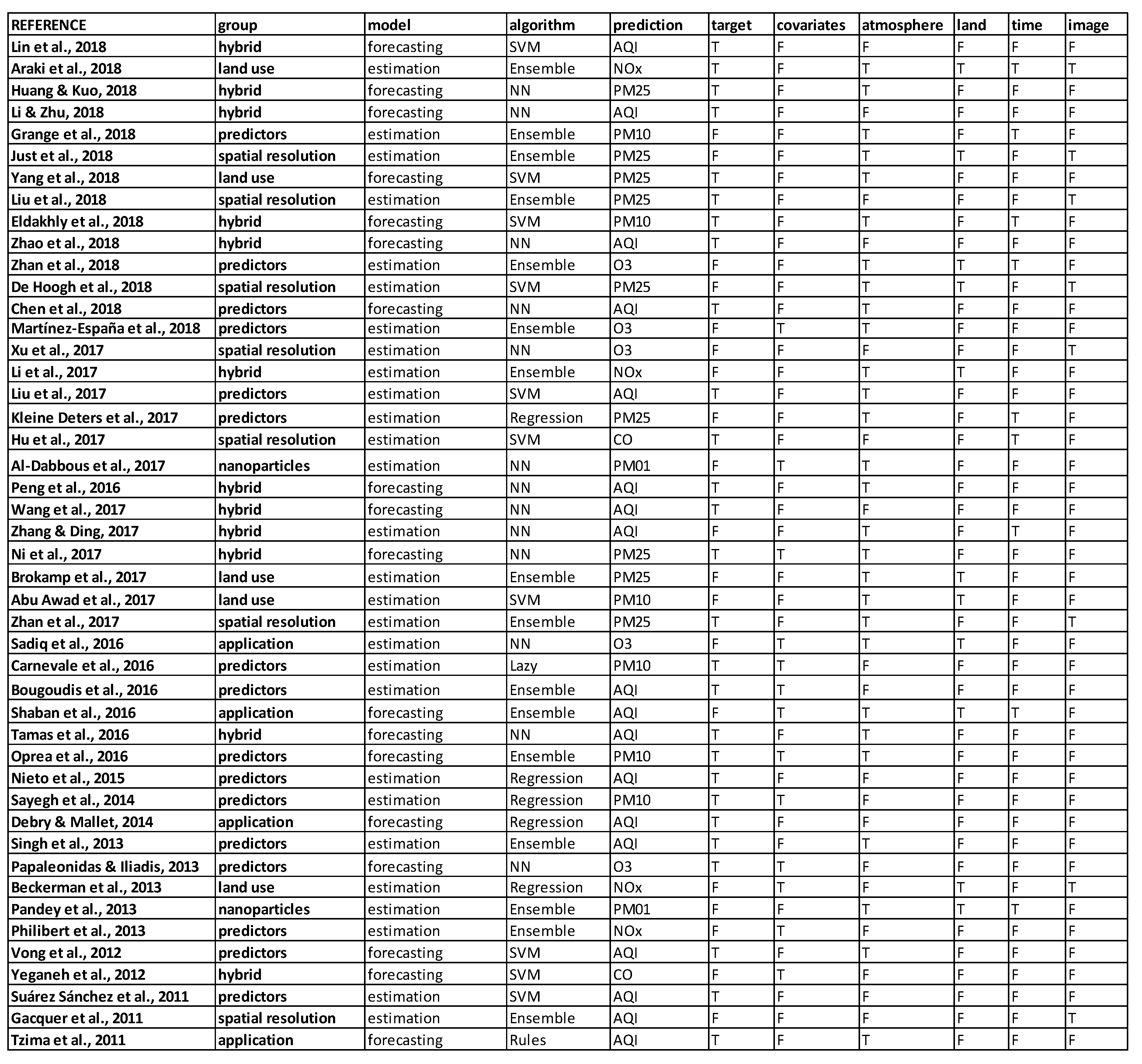
This section consists of a detailed explanation of the selected papers. It is organized into six categories based on the main motivation of the study. In each group, we first present manuscripts on estimation models and, second, studies that involve forecasting models. An estimation model is defined as an approach that seeks to estimate the value of a pollutant (or index of contamination) from the measurement of other predictive parameters at the same time step. It is mostly used to give an approximation of the concentrations on an extended geographic area. On the contrary, the objective of a forecasting model is to predict the concentration levels of the contaminants in the near future. We call both estimation and forecasting prediction or predictive models.
3.2.1. Category 1: Identifying Relevant Predictors and Understanding the Non-Linear Relationship with Air Pollution
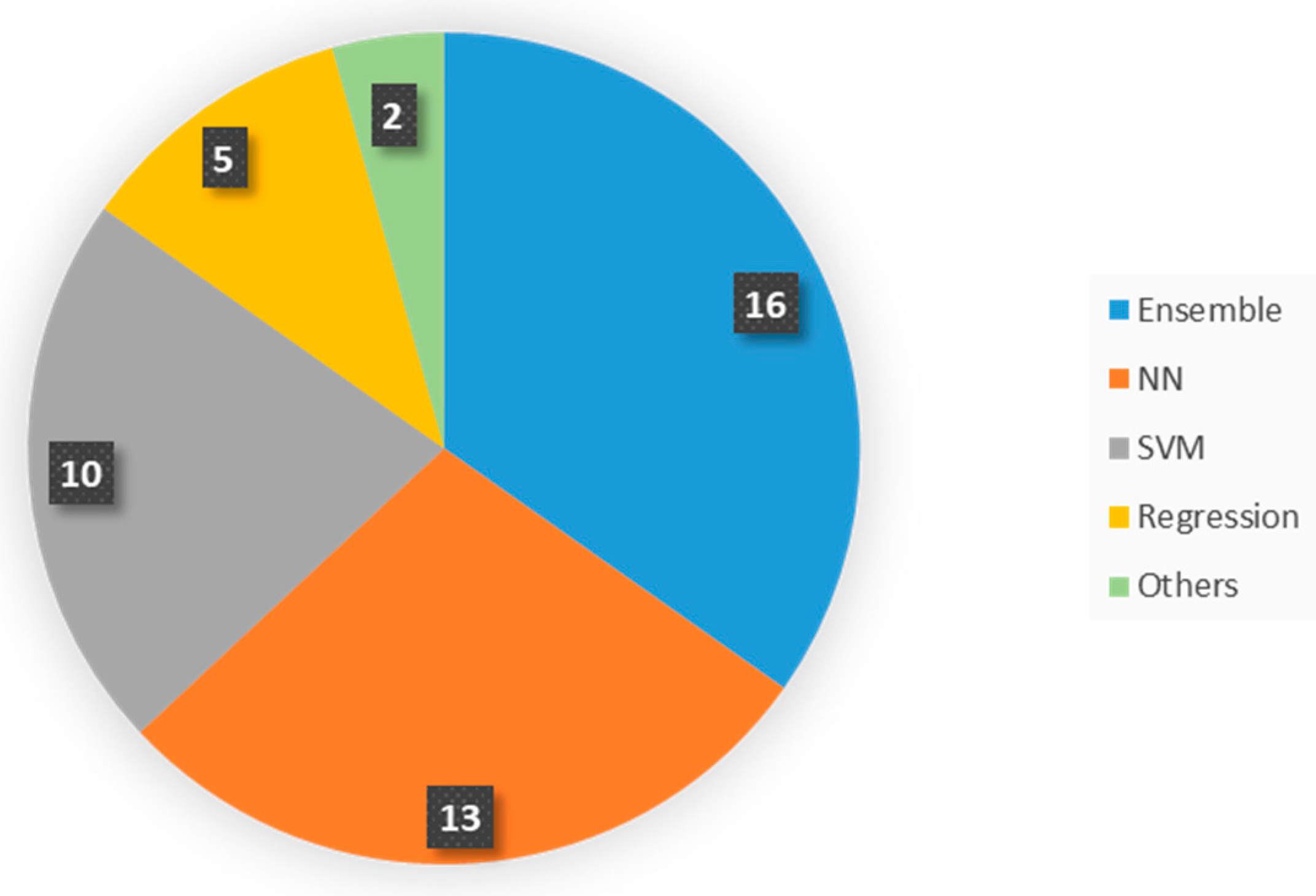
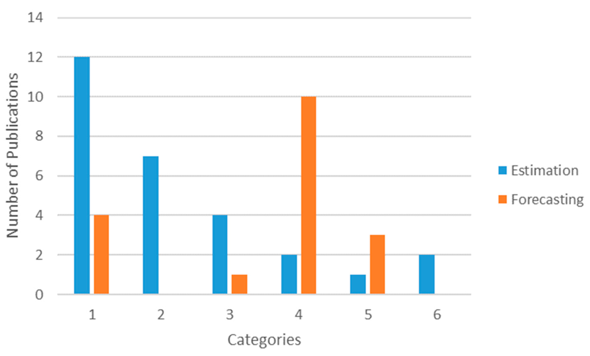
Category 1 is the biggest group and accounts for total of 16 articles—twelve in estimation modeling and four in forecasting. In the estimation modeling there are five cases of Random Forest (RF) or tree-based Ensemble learning algorithms (e.g., M5P), four regression models, one lazy learning, and two SVM. The latter was once used in forecasting studies, NN was used twice and M5P once. This category highly concentrates on identifying the most contributing parameters to a successful prediction of atmospheric pollution. A variety of tests are used to differentiate between the influential predictors, like Principal Component Analysis (PCA), Quantile Regression Model (QRM), Pearson correlation, etc.
Among the most recent studies we find Grange et al. [
22]. This study aims to (i) build a predictive model of PM
10 based on meteorological, atmospheric, and temporal factors and (ii) analyze PM
10 trend during the last ten years. The Random Forest model, a simple, efficient, and easy interpretable method, is used. First of all, many out-of-bag samples (randomly sampling observations with replacement and sampling of feature variables) of the training set are used to grow different Decision Trees (DT), and then all the trees are aggregated to form a single prediction. The algorithms are trained and run on 20 years of data in Switzerland from 31 monitoring stations. Daily average data of meteorology (wind speed, wind direction, and temperature), synoptic scale, boundary layer height, and time are used. The model is validated by comparison between the observed and predicted value, resulting in average value in 31 sites: r
2 = 0.62. The best predictors are—wind speed, day of the year (seasonal effect), and boundary layer height, whereas the worst predictors are day of the week, and synoptic scale. The model performance is low and the predictive accuracy is inconsistent (0.53 < r
2 < 0.71) for different locations, especially varying for the rural mountain sites.
Another study also relies on RF to build a spatiotemporal model to predict O
3 concentration across China [
35]. First the RF model is built by averaging the predictions from 500 decision/regression trees, and then Random Forest Regressor from the python package scikit-learn is used to run the algorithm. For that meteorology, planetary boundary height, elevation, anthropogenic emission inventory, land use, vegetation index, road density, population density, and time are used from 1601 stations over one year in all of China. The model is validated by comparison of the r
2 and RMSE (predicted value/actual value) to Chemical Transport Models, and shows a good performance of r
2 = 0.69 (specifically, r
2 = 0.56 in winter, and r
2 = 0.72 in fall). Interestingly, the model results are quite comparable or even higher than the predictive performance of the CTMs for lower computational costs. While for the predictive features, meteorological factors account for 65% of the predictive accuracy (especially humidity, temperature, and solar radiation), also showing a higher predictive performance when the weather conditions are stronger (i.e., autumn). In this study, anthropogenic emissions (NH
3, CO, Organic Carbon, and NO
x) exhibit a lower importance than meteorology and lower accuracy is registered for the regions with a sparser density of monitoring stations. Therefore, the accuracy relies on the complexity of the network.
Martínez-España et al. [
36] aim to identify the most robust machine learning algorithms to preserve a fair accuracy when O
3 monitoring failures may occur, by using five different algorithms—Bagging vs. Random Committee (RC) vs. Random Forest vs. Decision Tree vs. k-Nearest Neighbors (kNN). First, the prediction accuracy of the five machine learning algorithms is compared, then a hierarchical clustering technique is applied to identify how many models are needed to predict the O
3 in the region of Murcia, Spain. Two years of pollutant covariates (O
3, NO, NO
2, SO
2, NO
x, PM
10, C
6H
6, C
7H
8, and XIL) and meteorological parameters (temperature, relative humidity, pressure, solar radiation, wind speed and direction) are used. The model is validated by the comparison of the coefficient of determination (predicted value/actual value) between the five models. Random Forest slightly outperforms the other models (r
2 = 0.85), followed by RC (r
2 = 0.83), Bagging and DT (r
2 = 0.82) and kNN (r
2 = 0.78). The best predictors are NO
x, temperature, wind direction, wind speed, relative humidity, SO
2, NO, and PM
10. Finally, the hierarchical cluster shows that two models are enough to describe the studied regions.
Bougoudis et al. [
37] aim to identify the conditions under which high pollution emerges and to use a better generalized model. Hybrid system based on the combination of unsupervised clustering, Artificial Neural Networks (ANN) and Random Forest (RF) ensembles and fuzzy logic is used to predict multiple criteria pollutants in Athens, Greece. Twelve years of hourly data of CO, NO, NO
2, SO
2, temperature, relative humidity, pressure, solar radiation, wind speed and direction are used. Unsupervised clustering of the initial dataset is executed in order to re-sample the data vectors; while ensemble ANN modeling is performed using a combination of machine learning algorithms. The optimization of the modeling performance is done with Mamdani rule-based fuzzy inference system (FIS, used to evaluate the performance of each model) that exploits relations between the parameters affecting air quality. Specifically, self-organizing maps are used to perform dataset re-sampling, then ensembles of feedforward artificial neural networks and random forests are trained to clustered data vectors. The estimation model performance is quite good for CO (r
2 = 0.95, RF_FIS), NO (r
2 = 0.95, ensemble NN_FIS), NO and O
3 (r
2 = 0.91, RF) and SO
2 (r
2 = 0.78, ensemble regression).
Sayegh et al. [
38] also employ a number of models (Multiple Linear Regression vs. Quantile Regression Model (QRM) vs. Generalized Additive Model vs. Boosted Regression Trees) to perform a comparative study on the performance for capturing the variability of PM
10. At the contrary of the linear regression, which considers variables distribution as a whole, the QRM defines the contribution (coefficient) of the predictors for different percentiles of PM
10 (here 10 percentiles or quantiles are used) to estimate the weight of each feature. Meteorological factors (wind speed, wind direction, temperature, humidity), chemical species (CO, NO
x, SO
2), and PM
10 of the previous day data for one year from Makkah (Saudi Arabia) are used. The model performance is validated with observed data and the QRM model shows a better performance (r
2 = 0.66) in predicting hourly PM
10 concentrations due to the contribution of covariates at different quantiles of the dependent variable (PM
10), instead of considering the central tendency of PM
10.
Singh et al. [
39] aim to identity sources of pollution and predict the air quality by using Hybrid Model of Principal Components Analysis, Tree-based Ensemble Learning (Single Decision Tree (SDT), Decision Tree Forest (DTF) and Decision Tree Boost (DTB)) vs. Support Vector Machine Model. Five years of air quality and meteorological parameter data are used for Lucknow (India). SDT, DTF, DTB and SVM are used to predict the Air Quality Index (AQI), and Combined AQI (CAQI)), and to determine the importance of predictor features. The model performance is validated by a comparison between the models and with the observed data. Decision Tree models—SDT (r
2 = 0.9), DTF (r
2 = 0.95), and DTB at r
2 = 0.96) outperform SVM (r
2 = 0.89).
Philibert et al. [
40] aim to predict a greenhouse gas N
2O emission using Random Forest vs. Two Regression models (linear and nonlinear) by employing global data of environmental and crop variables (e.g., fertilization, type of crop, experiment duration, country, etc.). The extreme values from data are removed, excluding the boreal ecosystem; input variable features are ranked by importance; controlling number of input variables to result in better prediction. The model is validated by a comparison to the regression model and the simple non-linear model (10-fold cross validation). RF outperforms the regression models by 20–24% of misclassifications.
Meanwhile, Nieto et al. [
41] aim to predict air pollution (NO
2, SO
2 and PM
10) in Oviedo, Spain based on a number of factors using Multivariate Adaptive Regression Splines and ANN Multilayer Perceptron (MLP). Three years of NO
x, CO, SO
2, O
3, and PM
10 data modeling result in a good estimation of NO
2: r
2 = 0.85; SO
2: r
2 = 0.82; PM
10 r
2 = 0.75 when compared with observed data.
Kleine Deters et al. [
42] aim to identify the meteorology effects on PM
2.5, by predicting it using six years of meteorological data (wind speed and direction, and precipitation) for Quito, Ecuador in regression modeling. This is a good simplified technique and an economic option for the cities with no air quality equipment. The model gets validated by regression between observed and predicted PM
2.5, and by a 10-fold cross validation of predicted vs. observed PM
2.5, which shows that this method is a fair approach to estimate PM
2.5 from meteorological data. In addition, the model performance is improved in the more extreme weather conditions (most influential parameters), as previously seen in Zhan et al. [
35].
Carnevale et al. [
43] use the lazy learning technique to establish the relationship between precursor emissions (PM
10) and pollutants (AQI of PM
10) for the Lombard region (Italy), using hourly Sulfur Dioxide (SO
2), Nitrogen oxides (NO
x), Carbon Monoxide (CO), PM
10, NH
3 data for one year. The Dijkstra algorithm is deployed in the large-scale data processing system. Eighty percent of the data are used as an example set and 20% as validation set (every 5th cell). The validation phase of surrogate models is performed comparing the output to deterministic model simulations, not the observations. Constant, linear, quadratic and combination approximation based on elevation of the area (0, 1, 2 and all polynomial approximations) are applied. The performance of the model is very comparable (r
2 = 0.99–1) to the Transport Chemical Aerosol Model (TCAM), a model that is computationally much costlier, currently used in decision making.
Suárez Sánchez et al. [
44] on the other hand, aim to estimate the dependence between primary and secondary pollutants; and most contributing factors in air quality using SVM radial (Gaussian), linear, quadratic, Pearson VII Universal Kernels (PUK) and multilayer perceptron (MLP) to predict NO
x, CO, SO
2, O
3, and PM
10. Three years of NO, NO
2, CO, SO
2, O
3, and PM
10 data are used in Aviles, Spain. The model is 10-fold cross validated with the observed data, resulting in best performance using PUK for NO
x and O
3 (r
2 = 0.8).
Liu et al. [
23] also employ SVM to get the most reliable predictive model of air quality (AQI) by considering monitoring data of three cities in China (Beijing, Tianjin, and Shijiazhuang). Two years of last-day AQI values, pollutant concentrations (PM
2.5, PM
10, SO
2, CO, NO
2, and O
3), meteorological factors (temperature, wind direction and velocity), and weather description (ex. cloudy/sunny, or rainy/snowy, etc.) are used as predicting features. The dataset is split into a training set and testing set through a 4-fold cross validation technique. To validate the model performance, the results are compared to the observed data. The model performance is especially improved when the surrounding cities’ air quality information is included.
Vong et al. [
45] also use SVM to forecast air quality (NO
2, SO
2, O
3, SPM) from pollutants and meteorological data in Macau (China). The training is performed on three years of data and tested on one whole year and then just on January and July for seasonal predictions. The Pearson correlation is used to identify the best predictors for each pollutant and different kernels are used to test which of the predictors or models get the best results. The Pearson correlation is also employed to determine how many days of data are optimal for forecasting. The model performance is validated by comparison to the observed data resulting in best kernel—linear and RBF, in polynomial (summer), confirming that SVM performance depends on the appropriate choice of the kernel.
In the forecasting model category, there are two articles that use NN, and meteorology and pollutants as predicting features. Chen et al. [
46] aim to build a model that forecasts AQI one day ahead by using an Ensemble Neural Network that processes selected factors using PEK-based machine learning for 16 main cities in China (three years of data). First a selection of the best predictors (PM
2.5, PM
10, and SO
2) is performed, based on Partial Mutual Information (PMI), which measures the degree of predictability of the output variable knowing the input variable, and then the daily AQI value is predicted, through PEK-based machine learning, by using the previous day’s meteorological and pollution conditions. The model is validated by a comparison between actual and predicted value, resulting in an average value of r
2 = 0.58.
Meanwhile, Papaleonidas and Iliadis [
47] present the spatiotemporal modelling of O
3 in Athens (Greece) also using NN, specifically developing 741 ANN (21 years of data). A multi-layer feed forward and back propagation optimization are employed. The best results are conceived with three approaches—the simplest ANN, the best ANN for each case of predictions, and the dynamic variation of NN. The performance of the model is validated with the observed data and between NN approaches, resulting in r
2 = 0.799, performing the best for the surrounding stations. This approach is concluded as a good option for modeling with monitoring station data due to very common gaps.
Finally, Oprea et al. [
48] aim to extract rules for guiding the forecasting of particulate matter (PM
10) concentration levels using Reduced Error Pruning Tree (REPTree) vs. M5P (an inductive learning algorithm). The principal component analysis is used to select the best predictors, and then 27 months of eight previous-days of PM
10, NO
2, SO
2, temperature and relative humidity data are used to predict PM
10 in Romania. The validation is performed by comparing the results of two models with the observed values, concluding that M5P provides the more accurate prediction of the short-term PM
10 concentrations (r
2 = 0.81, for one day ahead and r
2 = 0.79 for two days ahead).
3.2.2. Category 2: Image-Based Monitoring and Tackling Low Spatial Resolution from Non-Specific/Low Resolution Sensors
This group is composed of a set of seven papers. All of them address estimation issues only. It is quite logical that no forecasting studies are included in this category, because the principal objective of this kind of work is to increase the spatial resolution of the current pollution spreading. To do so, a first paper presents a method to improve the spatial resolution and accuracy of satellite-derived ground-level PM
2.5 by adding a geostatistical model (Random Forest-based Regression Kriging—RFRK) to the traditional geophysical model (i.e., Chemical Transport Models—CTM) [
49]. This is a two-step procedure in which a Random Forest regression models the nonlinear relationship between PM
2.5 and the geographic variables (step 1) then the kriging is applied to estimate the residuals (or error) of step 1 (step 2). This work is carried out in the USA and is based on a 14 years dataset. The predictive features include CTM, satellite-derived dataset (meteorology and emissions), geographic variables (brightness of Night Time Lights—NTL, Normalized Difference Vegetation Index—NDVI, and elevation), and in situ PM
2.5. The accuracy is evaluated by comparing the RFRK to CTM-derived PM
2.5 models and using ground-based PM
2.5 monitor measurements as reference. The results show that the RFRK significantly outperforms the other models. In addition, this method has a relatively low computational cost and high flexibility to incorporate auxiliary variables. Among the three geographic variables, elevation contributes the most and NDVI contributes the less to the prediction of PM
2.5 concentrations. The main limitation of the technique is to rely on satellite images that are subject to uncertainties (e.g., data quality, completeness, and calibration).
A similar approach is proposed by Just et al. [
50]. The motivation of this study is to enhance satellite-derived Aerosol Optical Depth (AOD) prediction, by applying a correction based on three different Ensemble Learning algorithms: Random Forest, Gradient Boosting, and Extreme Gradient Boosting (XGBoost) The correction is implemented by considering additional inputs as predictive factors (e.g., land use and meteorology) than AOD only. This technique is applied to predict the concentration of PM
2.5 in Northeastern USA during a period of 14 years. The accuracy of the method is assessed by comparing the coefficient of determination (predicted value/actual value) between the three models. The result shows that XGBoost outperforms slightly the other two algorithms. In addition, the study demonstrates that including land use and meteorological parameters in the algorithms improves significantly the accuracy when compared to the raw AOD. Nevertheless, a limitation of the technique is the fact that it requires lots of features (total number = 52). Furthermore, Zhan et al. [
51] propose an improved version of the Gradient Boosting algorithm by considering the spatial nonlinearity between PM
2.5 and AOD and meteorology. They develop a Geographically-Weighted Gradient Boosting Machine (GW-GBM) based on spatial smoothing kernels (i.e., gaussian) to weight the optimized loss function. This model is applied to all China and uses data of 2014. The GW-GBM provides a better coefficient of determination than the traditional GBM. The study shows that the best features in descending order are: day of year, AOD, pressure, temperature, wind direction, relative humidity, solar radiation, and precipitation.
Xu et al. [
52] estimate ozone profile shapes from satellite-derived data. They develop a NN-based algorithm, called the Physics Inverse Learning Machine. The proposed method is composed of five steps. Step 1 is a clustering that gets groups of ozone profiles according to their similarity (k-means clustering procedure). Step 2 generates simulated satellite ultraviolet spectral absorption (UV spectra) of representative ozone profiles from each cluster. Step 3 consists of improving the classification effectiveness by reducing the input data through a Principal Component Analysis. In step 4 the classification model is applied for assigning an ozone profile class corresponding to a given UV spectrum. And in step 5 the ozone profile shape is scaled according to the total ozone columns. The algorithm is tested by comparing the predicted value to the observed value. 11 clusters are obtained, and the estimation error is lower than 10%. This technique can be considered an encouraging approach to predict ozone shapes based on a classification framework rather than the conventional inversion methods, even if its computational cost is relatively high.
A slightly different approach is proposed by de Hoogh et al. [
53]. This work aims to build global (1 km × 1 km) and local (100 m × 100 m) models to predict PM
2.5 from AOD and PM
2.5/PM
10 ratio. It is based on an SVM algorithm to predict the concentration of PM
2.5 in Switzerland. The dataset is composed of 11 years of observations and a broad spectrum of features, such as: Planetary boundary layers, meteorological factors, sources of pollution, AOD, elevation, and land use. The results show that the method is able to predict PM
2.5 by using data provided by sparse monitoring stations. Another technique consists of supplementing sparse accurate station monitoring by lower fidelity dense mobile sensors, with the aim of getting a fine spatial granularity [
54]. Seven Regression models are used to predict CO concentrations in Sidney, Australia. The study is divided into three stages. First, the models are built from seven years of historical data of static monitoring (15 stations) and three years of mobile monitoring. Second, the performances of each algorithm are compared. And third, field trials are conducted to validate the models. The results show that the best predictions are provided by Support Vector Regression (SVR), Decision Tree Regression (DTR), and Random Forest Regression (RFR). The validations on the field suggest that SVR has the highest spatial resolution estimation and indicates boundaries of polluted area better than the other regression models. In addition, a web application is implemented to collect data from static and mobile sensors, and to inform users.
Finally, a quite different study uses image processing to predict pollution from a video-camera analysis [
55]. Again, several families of machine learning algorithms are tested and compared. The method involves four sequential steps, which are: (i) camera records, (ii) image processing, (iii) feature extraction, and (iv) machine learning classification. The objective is to assess the severity of the pollution cloud emitted by factories from 12 features characterizing the image, such as— luminosity, surface of the cloud, color, and duration of the cloud. Although all the algorithms provide a similar performance, Decision Tree is the only one to be systematically classified among the models with the best (i) robustness of the parameter setting (= easy to configure), (ii) robustness to the size of the learning set, and (iii) computational cost. This study introduces interesting performance metrics based on ‘efficiency’ (higher weight for the correct classification of ‘critical events’ than ‘noncritical events’) instead of ‘accuracy’ (same weight for any event). In addition, with the objective to tackle the issue of unbalanced classes and since the authors are more interested in critical events (black cloud), which are less represented, some ‘noncritical events’ are removed from the learning set in order to get a balanced representation of the classes. Nevertheless, the application of this method is limited to the assessment of the contamination produced by plants.
3.2.3. Category 3: Considering Land Use and Spatial Heterogeneity/Dependence
Four out of five papers classified in this category are estimation models. The most general manuscript is written by Abu Awad et al. [
56]. The objective is to build a land use model to predict Black Carbon (PM
10) concentrations. The approach is divided into two steps. First, a land use regression model is improved by using a nu-Support Vector Regression (nu-SVR). Second, a generalized additive model is used to refit residuals from nu-SVR. This study is applied in New England States (USA) and exploits a 12 years dataset, which stores data from 368 monitoring stations. A broad spectrum of variables is used as features, such as: Filter analysis, spatial predictors (elevation, population density, traffic density, etc.), and temporal predictors (meteorology, planet boundary layer, etc.). The model is tested in cold and warm seasons and is assessed by comparison to actual data. Overall, the results provide a high coefficient of determination (r
2 = 0.8). In addition, it appears that this coefficient is significantly higher in the cold than in the warm season.
Araki et al. [
57] also build a spatiotemporal model based on land use to capture interactions and non-linear relationships between pollutants and land. The study consists of comparing two algorithms—Land Use Random Forest (LURF) vs. Land Use Regression (LUR)—to estimate the concentration levels of NO
2. This work takes place in the region of Amagasaki, in Japan, over a period of four years. Besides land use, the authors use population, emission intensities, meteorology, satellite-derived NO
2, and time as features. The accuracy of LURF outperforms slightly LUR, and the coefficient of determination gets a same range of values as in the above study. LURF is a bit better than LUR, because the former allows for a non-linear modelling whereas the latter is limited to a linear relationship. Another advantage of using random forest is to produce an automatic selection of the most relevant features. The results show that the best predictors in descending order are—green area ratio, satellite-based NO
2, emission sources, month, highways, and meteorology. The variable population is discarded from the model. Nevertheless, the interpretation of the regression model is easier than the random forest-based model, because the former provides coefficients representing the direction and magnitude of the effects of predictor variables. The variable selection issue related to LUR is tackled in the study carried out by Beckerman et al. [
58]. They develop a hybrid model that mix LUR with deletion, substitution, and addition machine learning. Thanks to this method, no more than 12 variables are used to predict the concentration of PM
2.5 and NO
2. The case study is applied to all California and uses data on the period 1999–2002 for PM
2.5, and 1988–2002 for NO
2. The overall performance of the model is fair, but the accuracy for estimating PM
2.5 is significantly lower than NO
2.
Brokamp et al. [
31] perform a deeper analysis based on a prediction of the concertation of the chemical composition of PM
2.5. As Beckerman et al. [
57], they compare the performance of a LURF versus LUR approach. The dataset is built from the measurements of 24 monitoring stations in the city of Cincinnati (USA) during the period 2001–2005. Over 50 spatial parameters are registered, which include transportation, physical features, socioeconomic characteristics, greenspace, land cover, and emission sources. Again, LURF outperforms slightly LUR. The originality of this work is to create models that predict not only the air quality, but also the individual concentration of metal components in the atmosphere from land use parameters.
Yang et al. [
59] is the only study of this category that provides a forecasting model. The approach is applied in three steps. First, a clustering analysis is performed to handle the spatial heterogeneity of PM
2.5 concentrations. Several clusters are defined, based on homogeneous subareas of the city of Beijing (China). Second, input spatial features that address the spatial dependence are calculated using a Gauss vector weight function. And third, spatial dependence variables and meteorological variables are used as input features of an SVR-based model of prediction. The performance of the proposed Space-Time Support Vector Regression (STSVR) algorithm is compared to the ARIMA, traditional SVR, and NN. The best model depends on the forecasting time span. STSVR outperforms the prediction of the other models from 1 h to 12 h ahead, whereas the global SVR outperforms STSVR from 13 h to 24 h ahead. This study demonstrates that (i) the relationship between air pollutant concentrations and other relevant variables changes over spatial areas, and (ii) as the forecasting time increases, the prediction accuracy decreases more with STSVR than SVR.
3.2.4. Category 4: Hybrid Models and Extreme/Deep Learning
This set of papers represents one of the rare categories in which forecasting models (10) are significantly more frequent than estimation models (2). The first estimation study consists of building a reliable model to predict NO
2 and NO
x with a high spatiotemporal resolution and over an extended period of time [
60]. This work is carried out in three steps. First, multiple non-linear (traffic, meteorology, etc.), fixed (e.g., population density) and spatial (e.g., elevation) effects are incorporated to characterize spatiotemporal variability of NO
2 and NO
x concentration. Second, the Ensemble Learning algorithm is applied to reduce variance and uncertainty in the prediction based on step 1. Third, an optimization process is implemented by tackling possible incomplete time-varying covariates recording (traffic, meteorology, etc.) in order to get a continuous time series dataset. The prediction performance is quite high (r
2 ≈ 0.85). Traffic density, population density, and meteorology (wind speed and temperature) account for 9–13%, 5–11%, and 7–8% of the variance, respectively. Nevertheless, the method is less accurate for the prediction of low pollution levels.
A different estimation approach is proposed by Zhang and Ding [
61]. The authors use an Extreme Learning Machine (ELM) to tackle the low convergence rate and the local minimum that characterize the NN algorithms. Their ELM consists of only 2-layer NN. The first layer (hidden layer) is fixed and random (its weight does not need to be adjusted). The second layer only is trained. They estimate a broad spectrum of contaminants (NO
2, NO
x, O
3, PM
2.5, and SO
2) from meteorological and time parameters. It appears that the ELM is significantly better than NN and Multiple Linear Regression (MLR), because it provides a higher accuracy and a lower computational cost. An even more advanced study is carried by Peng et al. [
62]. The authors propose an efficient non-linear machine learning algorithm for air quality forecasting (up to 48 h), which is easily updatable in ‘real time’ thanks to a linear solution applied to the new data. Five algorithms are compared: MLR, Multi-Layer Neural Network (MLNN), ELM, updated-MLR, and updated-ELM. This approach involves two steps and predict three types of contaminants (O
3, PM
2.5, and NO
2). Step 1 consists of the initial training stage of the algorithm. The 2nd step involves a sequential learning phase, in order to proceed with an online (daily) update of the MLR and ELM, and only seasonally (trimonthly) update of the MLNN. The results show that the updated-ELM tends to outperform the other models, in terms of R
2 and MAE. In addition, the linear updating applied to MLR and ELM is less costly than updating a MLNN. Nevertheless, all the models tend to underpredict extreme values (the non-linear models even more than the linear models).
Another type of forecasting involves hybrid models. This is the case of the study performed by Zhang et al. [
63], who predict short and long-term CO from a hybrid model composed with Partial Least Square (PLS), for data selection, and SVM, for modelling. Overall, SVM-PLS seems more performant than traditional SVM, because both the precision and computational cost of the former is better than the latter. However, the accuracy is lower for hourly than daily forecasting. Tamas et al. [
64] propose a different hybrid model to forecast air contaminants (O
3, NO
2, and PM
10), with a special focus on the critical prediction of pollution peaks. The hybrid model is composed with NN and clustering and it is compared to the Multilayer Perceptron. The proposed algorithm outperforms the traditional NN, especially in the prediction of PM
10 and O
3 peaks of pollution. Since performing a forecasting consists mainly of predicting a time series, Ni et al. [
65] propose a hybrid model that implements a NN and an Autoregressive Integrated Moving Average (ARIMA). The concentration of PM
2.5 are predicted in Beijing (China) from meteorological parameters, chemical variables, and microblog data. Such an approach allows for a good forecast for a few hours ahead, but the bigger the time lag, the bigger the error.
A time series analysis is also used by Li and Zhu [
66] to predict the AQI (NO
2 + PM
10 + O
3 + PM
2.5) 1 h ahead and from the extraction of conceptual features (randomness and fuzziness of time series data). A hybrid model based on a technique of Cloud Model Granulation (CMG) and SVR is implemented in two steps. First, CMG uses probability and fuzzy theory to extract from time series the concept features of: randomness and fuzziness of the data. And second, after extracting these features, an SVR is used for the prediction per se. The performance of CMG-SVR is slightly better than the individual application of the same techniques (CMG and SVR alone) or a NN. Nevertheless, this method is still only able to make a short-term prediction (about 1 h ahead). The fuzzy approach to forecast PM
10 hourly concentration 1 h ahead is also used by Eldakhly et al. [
67]. To tackle the randomness and fuzziness of the data, the hybrid model applies, first, a chance weight value to the target variable in order to minimize an outliner point (if any) that can be used, afterward, as a support vector point during the training process. The result of this study is one of the rare examples that shows a model that outperforms ensemble learning algorithms (Boosting and Stacking).
Wang et al. [
68] propose to optimize the AQI forecasting by applying a ‘decomposition and ensemble’ technique in three steps: (i) decomposition of the original AQI time series into a set of independent components (i.e., frequencies or IMFs), (ii) prediction of each component (by ELM), and (iii) aggregation of the forecast values of all components. The hybrid model takes every eight successive days as AQI data inputs of the ELM to forecast the ninth day. The originality of the study is to propose a decomposition of the AQI time series into two phases— by Complementary Ensemble Empirical Mode Decomposition (CEEMD), for low and medium frequencies, and by Variation Mode Decomposition (VMD), for high frequencies. This 2-phase decomposition provides a superior forecasting accuracy than 1-phase decomposition implementations. Fuzzy logic, ELM, and heuristic are put together in the model developed by Li et al. [
66]. This study forecasts the AQI (based on PM
10, PM
2.5, SO
2, NO
2, CO, and O
3) of six cities in China. Fuzzy logic is used as a feature selection, because relevant predictive contaminants are not the same according to the city. ELM and heuristic optimization algorithms are applied for a deterministic prediction of the contaminant concentrations. This hybrid model gives a better prediction than other NN and time series (e.g., ARIMA) algorithms but it is slightly slower than the NNs.
More recently, a bunch of studies have implemented a Deep Learning approach to improve the accuracy of air pollution forecasting. For instance, Zhao et al. [
69] propose a Deep Recurrent Neural Network (DRNN) method to forecast daily Air Quality Classification (AQC). This technique is divided into two steps. First, data of six pollutants are pre-processed, in order to group the concentrations into four categories or Individual Air Quality Index—IAQI (from unhealthy to good). Second, an RNN based on Long Short-Term Memory (LSTM) is used to perform the forecasting. LSTM is an RNN, which includes a memory that permits to learn the input sequence with longer time steps (e.g., problems related to time series). Despite the high expectations, the predictive accuracy of the model is not significantly better than the performance of the other tested algorithms (SVM and Ensemble Learning). In addition, the disadvantage of Deep Learning is a high computational cost and a low interpretability of the model. A more satisfactory result is obtained by Huang and Kuo [
70], who also use a hybrid model based on NN and LSTM to forecast PM
2.5 concentrations 1 h ahead, by processing big data. The authors use a Convolutional Neural Network (CNN) instead of the traditional NN, because its partially connected architecture allows for a reduced training time. This optimized model seems to outperform all the principal machine learning algorithms (SVM, Random Forest, and Multilayer Perceptron). However, the relevance of such a technique still has to be confirmed over a longer time span forecast.
3.2.6. Category 6: Nanoparticles as a New Challenge
In the last category, the studies focus on estimating the concentrations and peaks of nanoparticles. A number of years of research indicates that the levels of PM
2.5 concentrations are dropping in most of the high- and mid-income countries [
75,
76,
77,
78]. However, in the case of nanoparticles, the harm comes not from their mass (particle concentration, usually high for the larger size aerosols), which compared to micro-sized particles is minute, but the quantity (particle number, usually very high for the smaller size aerosols) entering the human blood stream and damaging the cardiovascular system. Recent study indicates that nanoparticles attack the injured blood vessels and may cause heart attacks and strokes, while long-term exposure causes vascular damage [
79]. Therefore, studying these ultrafine particles (UFP) is quite important due to the increased production of very small particles by modern engines. However, not many cities have the infrastructure to monitor these complex pollutants. Therefore, Al–Dabbous et al. [
80] aim to build a model that estimates the concentration of nanoparticles from accessible and routinely-monitored pollution and meteorological factors using a feed-forward Neural Network with back-propagation. First, different architectures of NN (number of layers and neurons) are tested through an empiric approach (i.e., trial and error), in order to select the models that provide the minimum error of prediction according to the features considered, then the seven best models (each one with different types and number of features) are compared, and finally, in order to assess the prediction of the models for high-pollution concentrations 75th percentile values are considered. One month of five pollutant covariates (PM
10, SO
2, O
3, NO
x, and CO), and/or meteorological data (wind speed, and temperature) are used in Fahaheel City (Kuwait). The model performance is assessed by comparison between the seven models (i.e., type and number of features considered) based on the determination coefficient. The models that include meteorology have the best results r
2 = 0.8 (with meteorology), and r
2 = 0.74 (without meteorology). The accuracy of the models is slightly lower for extreme concentrations (>75th percentile values). The study shows that the concentration in nanoparticles is very sensitive to meteorological factors.
Similarly, Pandey et al. [
81] aim to understand the relationships between the concentration of submicron particles and meteorological and traffic factors in order to estimate nanoparticles (particulate matter less than 1 µm—PM
1, and UFP) in Hangzhou (China). As in the previous study [
80], a short term, three days in winter data of meteorological (temperature, relative humidity, wind speed and direction, precipitation and pressure), traffic (flow, speed) and time parameters are used. Tree-based classification models, SVM, Naïve Bayes, Bayesian Network, NN, k-NN, Ripper and RF are implemented. Correlation with PM and each predictor is performed, to know which single feature has better predicting power, and based on that the multiple parameter model is used. Data are split into two (low vs. high) and three (low vs. medium vs. high) ranges of pollution classes. Model performance is validated against the observed data (precision, area under curve—AUC) resulting in tree algorithm AUC and f-measure 1 for PM
1 (ADTree, RF), and for UFP 0.84 (RF). This study is a promising example in predicting nanoparticles without actual measurements. It shows that it is easier to predict PM
1, than UFP. Tree algorithms are able to produce almost completely accurate prediction of PM
1, and very good (r
2 = 0.844) for UFP. A binary split is better than ternary for all classifiers. Finally, weather also shows a strong relationship with PM
1, while traffic parameter is important for UFP.


