Salient Region Detection Using Diffusion Process with Nonlocal Connections

Abstract

Diffusion-based salient region detection methods have gained great popularity. In most diffusion-based methods, the saliency values are ranked on 2-layer neighborhood graph by connecting each node to its neighboring nodes and the nodes sharing common boundaries with its neighboring nodes. However, only considering the local relevance between neighbors, the salient region may be heterogeneous and even wrongly suppressed, especially when the features of salient object are diverse. In order to address the issue, we present an effective saliency detection method using diffusing process on the graph with nonlocal connections. First, a saliency-biased Gaussian model is used to refine the saliency map based on the compactness cue, and then, the saliency information of compactness is diffused on 2-layer sparse graph with nonlocal connections. Second, we obtain the contrast of each superpixel by restricting the reference region to the background. Similarly, a saliency-biased Gaussian refinement model is generated and the saliency information based on the uniqueness cue is propagated on the 2-layer sparse graph. We linearly integrate the initial saliency maps based on the compactness and uniqueness cues due to the complementarity to each other. Finally, to obtain a highlighted and homogeneous saliency map, a single-layer updating and multi-layer integrating scheme is presented. Comprehensive experiments on four benchmark datasets demonstrate that the proposed method performs better in terms of various evaluation metrics.

1. Introduction

Saliency detection, which aims to find the most noteworthy region in a scene, is becoming increasingly important, especially when the amount of image is explosively increasing in the age of Big Data. It has been effectively applied in many computer vision tasks, such as image segmentation [1], object detection and recognition [2,3], and image compression [4].

Many saliency detection methods have been proposed. These models can generally be categorized into top-down and bottom-up methods in terms of the mechanisms. Top-down methods [5,6] are task-driven which generally require supervised learning and need to exploit high-level human perceptual knowledge. Bottom-up methods [7,8,9,10,11,12,13,14,15] are data-driven and usually exploit low-level cues, such as features, colors, and spatial distances to construct saliency maps. Most bottom-up methods adopt compactness [8,9,16], uniqueness [7,13,14,15], and background cues [10,11,12].

Most compactness-based methods [8,9,16] consider the spatial variance of features. Generally, salient region has a low compactness variance due to the tight distribution, whereas the feature of background is distributed over the entire image, which means the higher compactness variance. However, the background regions may be wrongly highlighted, especially when the feature of background also has a compact distribution.

Contrast to the compactness-based methods, the most uniqueness-based methods, consider the difference between image pixels or regions. According to the contrastive reference regions, these methods can be roughly divided into local and global contrast-based methods. Local contrast-based methods [13,14] obtain the uniqueness of pixels or regions with respect to their neighborhoods, while global contrast-based methods [7,15] restrict the reference regions to the entire image. However, the local contrast-based methods tend to highlight the edges of salient region rather than the whole salient region, while the global contrast-based methods are inclined to emphasize the entire image in some cases.

Background-based methods [10,11,12] construct the saliency map via considering the location property of the background region in the image. On the contrary, center prior directly introduces the location prior knowledge of the salient object itself. But substantially, both of them are the explanations of feature distribution in the spatial dimension, and they are both motivated by the psychophysical observations that salient objects seldom touch the image boundary, whereas the background regions can be easily connected to the boundary. However, the background prior may be ineffective because the salient regions do not always appear at the center of image.

Although the above-mentioned methods have achieved good performances in some respects, every low-level cue has its own limitations. To address these issues, many combined algorithms are proposed. Diffusion-based methods [9,16,17,18,19,20,21,22,23,24,25,26,27,28,29,30,31,32,33,34,35,36], which propagate the saliency information on the graph, are one of the effective methods. Liu et al. [18] constructed a conditional random field to combine multiple features for salient object detection. Ren et al. [20] applied a Gaussian Mixture Model (GMM) to cluster superpixels, and calculated the saliency value using compactness metric with modified PageRank propagation. Mai et al. [21] presented a data-driven approach to aggregate the saliency that generated by multiple individual saliency detection methods using a conditional random field. Gopalakrishnan et al. [22] formulated the problem of salient object detection in images as an automatic labeling problem on the vertices of a weighted graph. Yang et al. [23] ranked the similarity of the image elements (pixels or regions) with foreground cues or background cues via graph-based manifold ranking. Jiang et al. [24] set virtual boundary nodes as the absorbing nodes in a Markov chain, and computed the absorbed time from transient node to absorbing nodes as the metric of saliency value. Lu et al. [26] proposed a method to learn optimal seeds for object saliency via combining the low-level and mid-level vision features. Sun et al. [27] exploited the relationship between the saliency detection and the Markov absorption probability to construct the saliency map. Jiang et al. [28] used the most dominant eigenvectors to re-synthesize the diffusion matrix and construct the seed vector based on the correlations of diffusion maps between the non-border nodes. Li et al. [29] proposed the regularized random walks ranking to formulate pixel-wised saliency maps from the superpixel-based background and foreground saliency estimations. Qin et al. [30] introduced the Cellular Automata mechanism into saliency detection via analyzing the intrinsic relevance of similar regions through interactions with neighbors. Li et al. [31] devised a co-transduction algorithm to fuse both boundary and object labels based on an inter propagation scheme. Gong et al. [32] employed the Teaching-to-Learn and Learning-to-Teach strategies to logically propagate the unlabeled superpixels from simple to difficult. Xiang et al. [34] propagated the background-driven saliency information on an optimized graph. Zhou et al. [9] proposed a bottom-up salient region detection diffusion-based method by integrating compactness and local contrast cues. Zhou et al. [16] propagated the saliency and background seed vectors on a two-layer sparse graph. Most above-mentioned diffusion-based methods ranked the saliency values on 2-layer neighborhood graph (or 2-layer sparse graph) by connecting each node to its neighboring nodes and the nodes sharing common boundaries with its neighboring nodes (or the most similar node that shares a common boundary with its neighboring nodes). In other words, most of them merely exploited the intrinsic relevance of local regions via measuring the similarities between each other. However, when the neighborhood nodes of salient regions are inhomogeneous or incoherent, the local connective weights, which are supposed to have a high value, may be low. Thus, the saliency information may be ranked with an inaccurate connective weight. Naturally, as shown in Figure 1, the inner salient region may be inhomogeneous, and the background may be wrongly highlighted.

In this paper, we put forward an effective method to overcome these issues. In term of the local relevance, the 2-layer sparse graph is adopted to optimize the local connections as well as [16], which is conducted by connecting each node to its neighboring nodes and the most similar node that shares a common boundary with its neighboring nodes. In term of the nonlocal relevance of different elements, we extend the nonlocal intrinsic relevance into the 2-layer sparse graph by connecting each node to the “true-foreground” and “true-background” seeds. As shown in Figure 2f, our proposed graph can effectively highlight the salient regions with a consistent value. What is more, the use of the nonlocal connections can effectively improve the performances of 2-layer neighborhood graph, which can be illustrated in Figure 2d. Second, to address the defect of the center-biased Gaussian model, we design a saliency-biased Gaussian model to refine the initial saliency maps generated by the compactness and uniqueness cues. Finally, a single-layer updating and multi-layer integrating scheme is generated to highlight the salient regions and make full use of the multi-scale saliency information.

The contributions of our paper can be summarized as follows:

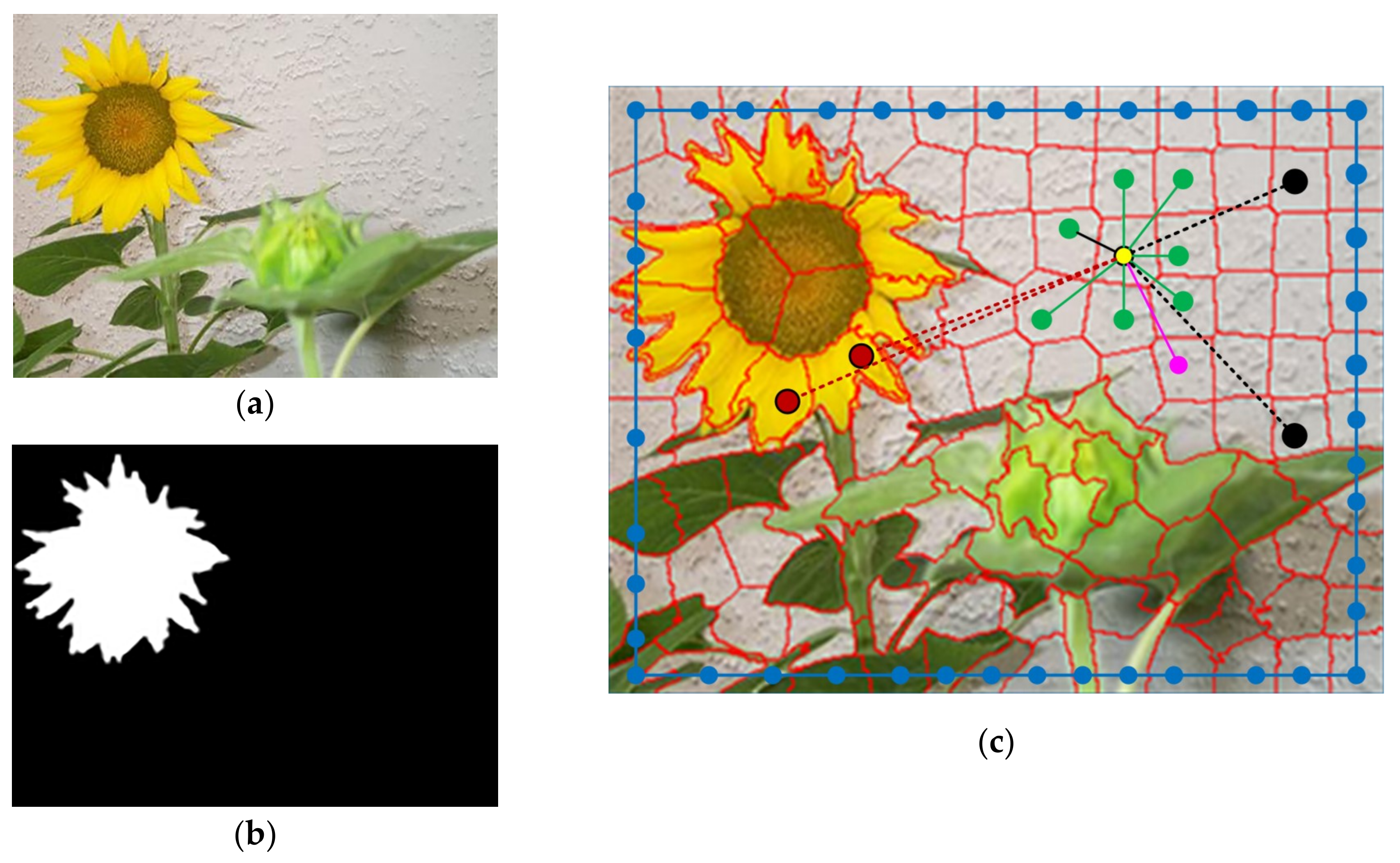
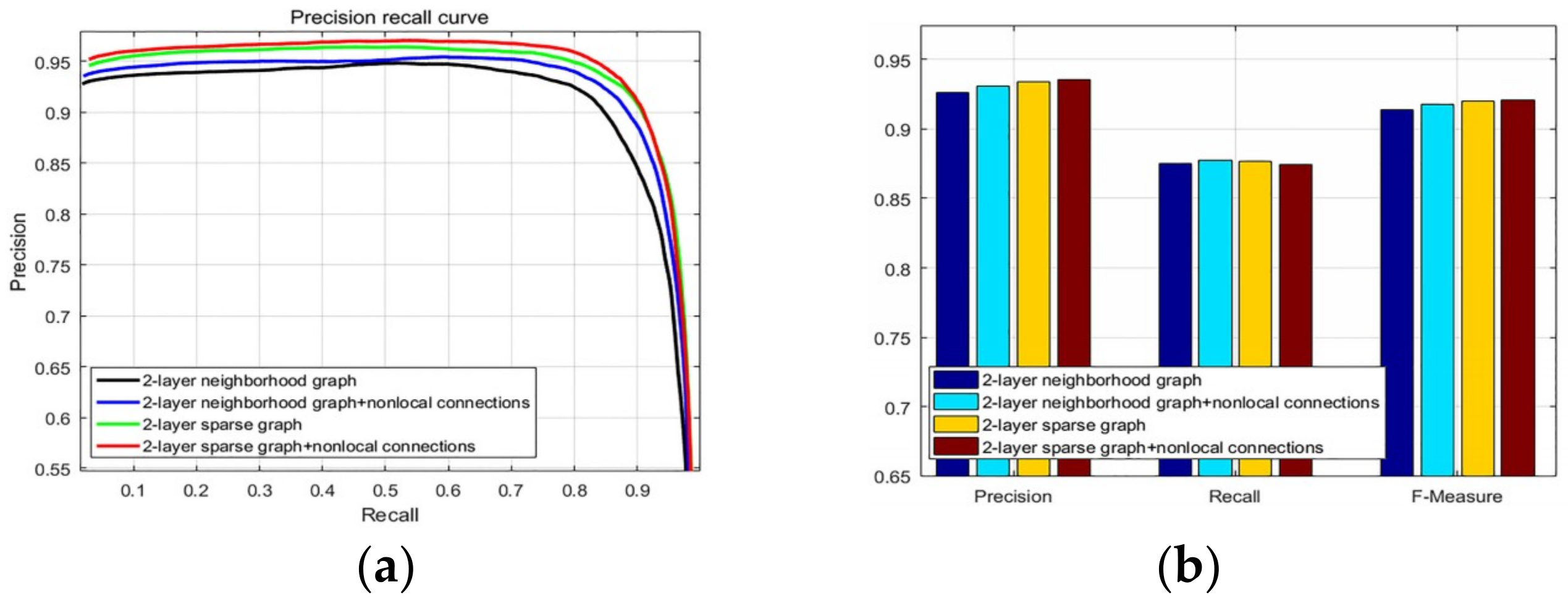
• The nonlocal intrinsic relevance is exploited into the 2-layer sparse graph, and with the saliency information based on different feature cues, we construct the new foreground and background biased diffusion matrix.
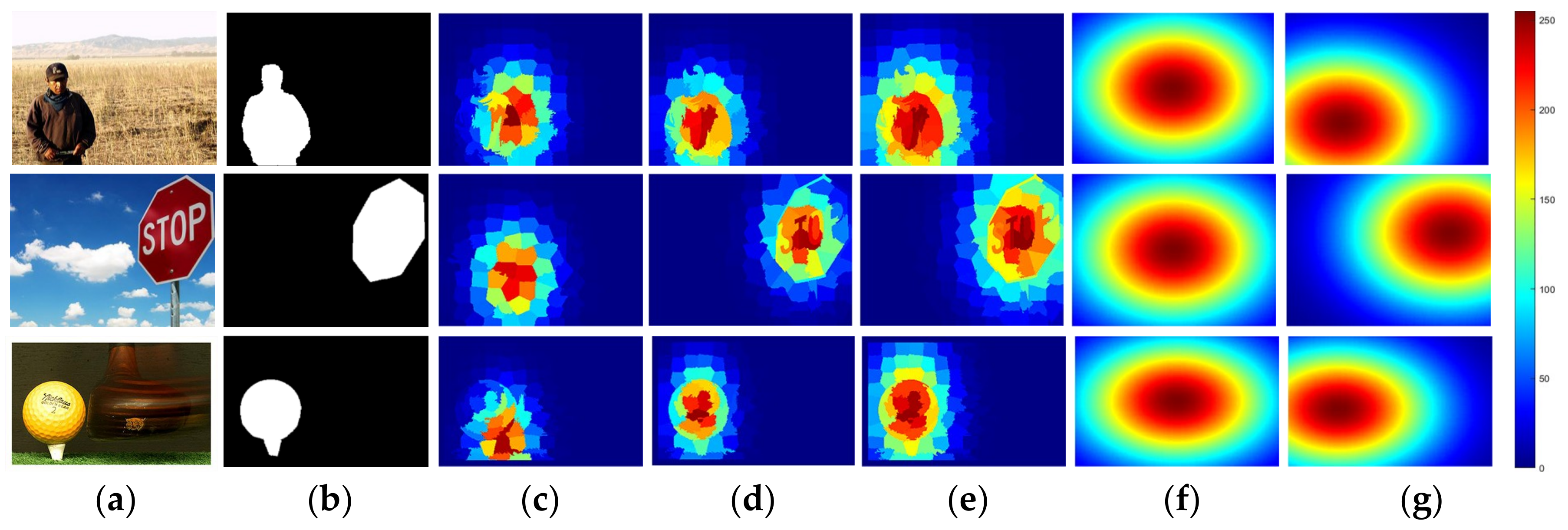
• A saliency-biased Gaussian model is presented to overcome the defect of the center-biased model.
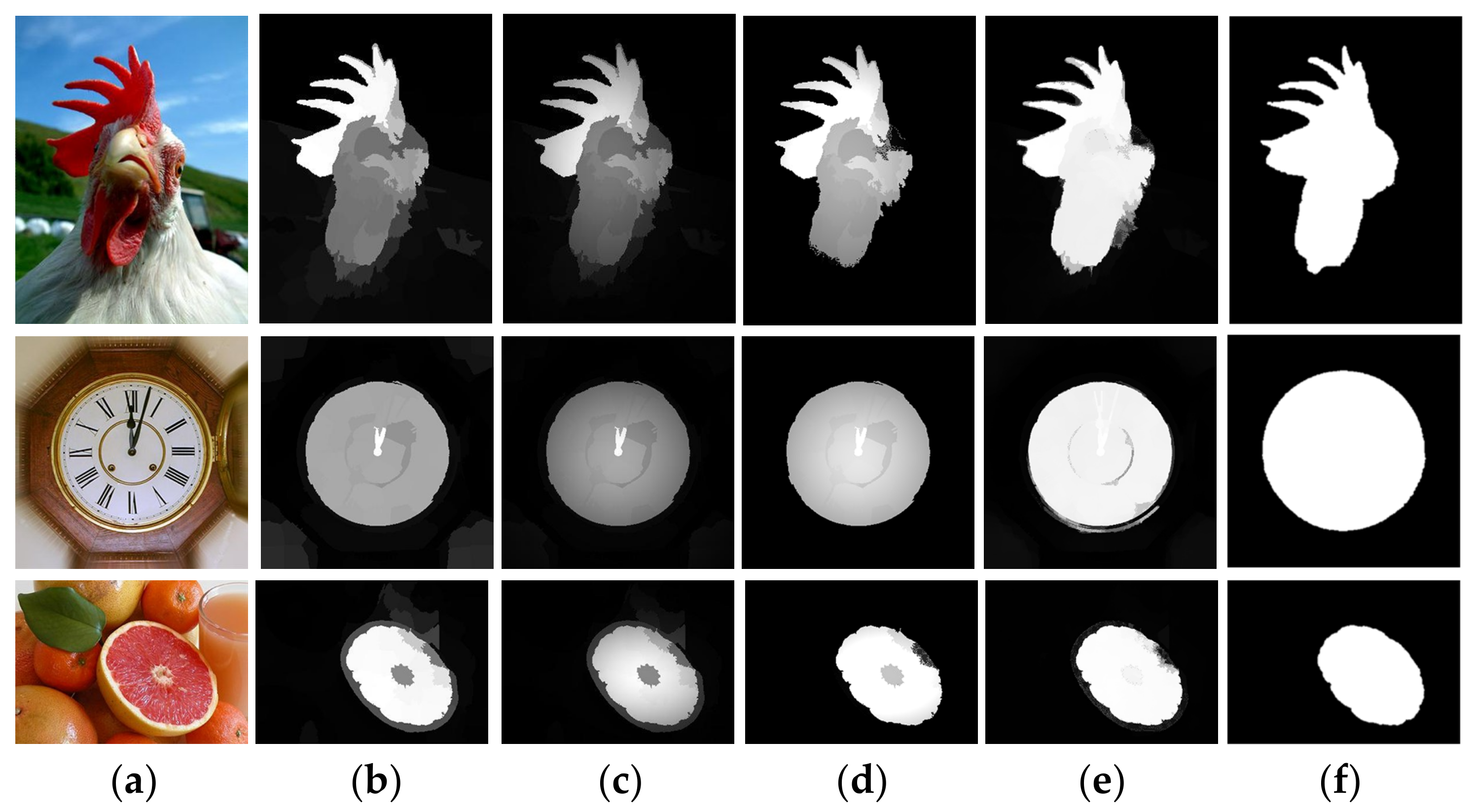
• To preferably highlight the salient regions and excavate the multi-scale saliency information, we design a single-layer updating and multi-layer integrating algorithm.

The remainder of this paper is organized as follows. In Section 2, we elaborate the proposed saliency detection method. In Section 3, extensive experiments are executed to evaluate the proposed approach with comparisons to the state-of-the-art methods on four datasets. In Section 4, we analyze the limitation of our method. In Section 5, we conclude this paper.

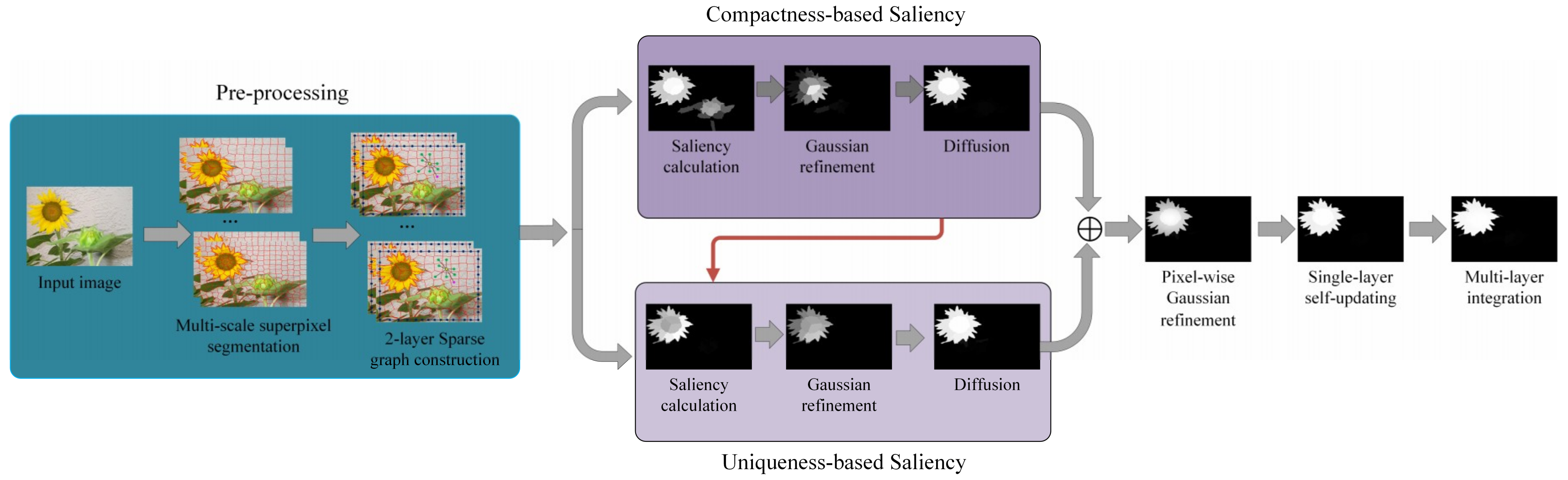
2. Proposed Approach

In this section, our proposed approach is presented in detail, the process of which is shown in Figure 3. First of all, to improve the robustness of multi-scale salient regions, we use the SLIC (simple linear iterative clustering) model [37] to abstract the input image into uniform and compact regions at five scales. Second, a saliency-biased (compactness-biased) Gaussian model is constructed to refine the initial saliency maps generated by the compactness cue, and then, the compactness information is diffused on the 2-layer sparse graph with the nonlocal connections. Similarly, the uniqueness-biased Gaussian model is formed, and the uniqueness information is propagated on the 2-layer sparse graph (without the nonlocal connections). Finally, we put forward a single-layer updating and multi-layer integrating scheme to obtain a more homogeneous salient region.

2.1. 2-Layer Sparse Graph Construction

After abstracting the image, the superpixels are mapped into a graph $G = (V,E)$ with N nodes $V=\left\{v_i|1\le i\le N\right\}$, and edges $E=\left\{e_{ij}|1\le i,j\le N\right\}$. Node $v_i$ corresponds to the image superpixels and edge $e_{ij}$ links nodes $v_i$ and $v_j$ to each other with an affinity matrix $W={[w_{ij}]}_{N\times N}$. In this paper, as proposed in [16], a 2-layer sparse graph is adopted. As shown in Figure 4, the graph is generated by connecting each node to its neighboring nodes and the most similar node sharing a common boundary with its neighboring nodes. As is illustrated in Figure 2, contrast to the 2-layer neighborhood graph, the 2-layer sparse graph can effectively avoid the disturbances of the dissimilar redundant nodes. In addition, the nodes on four sides are connected and any pair of boundary nodes are considered to be adjacent as well as [23,24,27].

In this paper, we define the weight $w_{ij}$ of edge $e_{ij}$ in 2-layer sparse graph as:

$$w_{ij}=\{\begin{array}{cc}{e}^{-\frac{\left|\right|l_i-l_j\left|\right|}{{\sigma }^2}}\hfill & \mathrm{if} \mathrm{node} v_i is \mathrm{connected} \mathrm{with} v_j\\ 0\hfill & \mathrm{others}\end{array}$$

(1)

where $\left|\right|l_i-l_j\left|\right|$ is the Euclidean Distance between the node $i$ and $j$ in CIELAB color space. $\sigma$ is a parameter controlling strength of the weight. We define the affinity matrix of the graph as $W={[w_{ij}]}_{N\times N}$, and a degree matrix $D = \mathrm{diag}\left\{d_{11},d_{22},\dots ,d_{NN}\right\}$ is generated, where $d_{ii}={\displaystyle {{\displaystyle \sum }}_j{w}_{ij}}$.

2.2. Compactness-Based Saliency Map

2.2.1. Compactness Calculation

Compactness is the measurement of the spatial variance of low-level feature. In [8], the compactness is defined as:

$$D_i={\displaystyle {\displaystyle \sum }_{j=1}^N\left|\right|p_j-{\mu }_i|{|}^{2}w(c_i,c_j)}$$

(2)

where $w(c_i,c_j)$ describes the similarity of color $c_i$ and color $c_j$ of segments $i$ and $j$,$p_j$ is again the position of segment $j$, and ${\mu }_i={\displaystyle {{\displaystyle \sum }}_{j=1}^{N}w(c_i,c_j)p_j}$ defines the weighted mean position of color $c_i$.

In this paper, we adopt the similar constituents with the Equation (2). However, instead of defining $w_{ij}$ as a Gaussian filtering function, we explain the similarity using:

$$a_{ij}=e^{-\frac{\left|\right|l_i-l_j\left|\right|}{{\sigma }^2}}$$

(3)

As proposed in [16], in order to describe the similarity more precisely, we propagate the similarity using manifold ranking [9] on the 2-layer sparse graph:

$$S={(D-\alpha W)}^{-1}A$$

(4)

where $A={\left[a_{ij}\right]}_{N\times N}$, $S={\left[s_{ij}\right]}_{N\times N}$ is the similarity matrix after the diffusion process, and $\alpha$ specifies the relative contributions to the ranking scores from the neighbors and the initial ranking scores.

As proposed in [16], we finally define the compactness as:

$$ComVal(i)=\frac{{\displaystyle {\displaystyle \sum }_{j=1}^N\left|\right|p_j-{\mu }_i\left|\right|\cdot s_{ij}\cdot n_j}}{{\displaystyle {{\displaystyle \sum }}_{j=1}^N{s}_{ij}\cdot n_j}}$$

(5)

where $n_j$ is the number of pixels that belong to superpixel $v_j$, $p_j=\left[p_j^x,p_j^y\right]$ is the centroid of the superpixel $v_j$, and ${\mu }_i=[{\mu }_i^x,{\mu }_i^y]$ is defined as:

$${\mu }_i^x=\frac{{\displaystyle {{\displaystyle \sum }}_{j=1}^N{s}_{ij}\cdot n_j\cdot p_j^x}}{{\displaystyle {{\displaystyle \sum }}_{j=1}^N{s}_{ij}\cdot n_j}}$$

(6)

Similarly, ${\mu }_i^y$ is defined as:

$${\mu }_i^y=\frac{{\displaystyle {{\displaystyle \sum }}_{j=1}^N{s}_{ij}\cdot n_j\cdot p_j^y}}{{\displaystyle {{\displaystyle \sum }}_{j=1}^N{s}_{ij}\cdot n_j}}$$

(7)

Salient regions generally have a low compactness value due to the concentrated distribution, whereas the background regions usually spread over the whole image, which means a high compactness value. Therefore, we calculate the initial saliency map using:

$$ComSal(i)=1-norm(ComVal)$$

(8)

The superpixels can be roughly divided into foreground seeds and background seeds based on the mean value of $ComSal$. We refer the two cluster sets of foreground seeds and background seeds as $\mathit{FG}$ and $\mathit{BG}$, respectively.

2.2.2. Compactness-Biased Gaussian Model

Center-prior introduces the location prior knowledge of the salient object. It is inspired by the observation that salient object always appears at the center of image. In [38,39], center prior has been used in the form of Gaussian model:

$$G(i)=\exp \left[-\left(\frac{{(x_i-{\mu }_x)}^2}{2{\sigma }_x^2}+\frac{{(y_i-{\mu }_y)}^2}{2{\sigma }_y^2}\right)\right]$$

(9)

where $x_i$ and $y_i$ are the central coordinates of the superpixel $v_i$, ${\mu }_x$ and ${\mu }_y$ represent the coordinates of the image center. However, as Figure 5c shows, the center-biased Gaussian model is not effective and may wrongly highlight the background. Inspired by [12], we present the compactness-biased Gaussian model as follows:

$$G_{com}(i)=\exp \left[-\left(\frac{{(x_i-w_x)}^2}{2{\sigma }_x^2}+\frac{{(y_i-w_y)}^2}{2{\sigma }_y^2}\right)\right]$$

(10)

where $w_x,w_y$ are defined as:

$$\{\begin{array}{l}{w}_x=\frac{{\displaystyle {{\displaystyle \sum }}_{i=1}^{N_{FG}}ComSal(i)}\cdot x_i}{{\displaystyle {{\displaystyle \sum }}_{i=1}^{N_{FG}}ComSal(i)}}\\ w_y=\frac{{\displaystyle {{\displaystyle \sum }}_{i=1}^{N_{FG}}ComSal(i)\cdot y_i}}{{\displaystyle {{\displaystyle \sum }}_{i=1}^{N_{FG}}ComSal(i)}}\end{array}$$

(11)

where $N_{FG}$ is the number of the superpixel in the foreground seeds. To avoid the disturbances of the background seeds, we merely choose the foreground seeds to participate in calculation. We set ${\sigma }_x= 0.15\times H$ and ${\sigma }_y=0.15\times W$, where $W$ and $H$ respectively denote the width and height of the image. Figure 5d shows the effects of the proposed compactness-biased Gaussian model. As it is illustrated, compared to the general Gaussian model, the proposed model is more precise to highlight the salient regions and suppress the background regions.

With the compactness-biased Gaussian model, we refine the initial saliency map generated by Equation (8):

$$S_{Gauss\_Com}(i)=ComSal(i)\cdot G_{com}(i)$$

(12)

We obtain the final compactness-based saliency map using the similarity $a_{ij}$ as the weight of the linear combination:

$$S_{fg\_com}(i)={\displaystyle {\displaystyle \sum }_{v_j\in FG}{S}_{Gauss\_Com}(j)\cdot a_{ij}}$$

(13)

2.2.3. Diffusion Process with Nonlocal Connections

As shown in Figure 2, the variance of feature in the foregrounds may lead to the variance of the saliency value, which may result in the inconsistency of salient regions. To address this issue, many diffusion-based models have been presented [9,16,17,18,19,20,21,22,23,24,25,26,27,28,29,30,31,32,33,34,35,36]. But most of them merely exploit the local intrinsic relevance on the graph. However, the weights between the local relevance may be inaccuracy, especially when the features of the salient regions have a complex distribution, after the diffusion process which is constructed only with local connections, the incorrect weights on the graph will inevitably lead to the suppression of the partial salient regions, which can be illustrated in Figure 2. Inspired by [36], we present a new diffusion model with nonlocal connections to address this issue.

In Section 2.2.1, we have roughly divided the superpixels into the foreground seeds and the background seeds. To find the more accurate foreground seeds and background seeds, we generate the “true-foreground” and “true-background” seed sets which are respectively referred as ${\mathit{T}}_{\mathit{f}}{, \mathit{T}}_{\mathit{b}}$ using:

$$\{\begin{array}{l}{\mathit{T}}_{\mathit{f}}=\left\{v_i|ComSal(i)\ge 0.9,i=1,2,\cdots ,N\right\}\\ {\mathit{T}}_{\mathit{b}}=\left\{v_i|ComSal(i)\le 0.1,i=1,2,\cdots ,N\right\}\end{array}$$

(14)

As Figure 4 shows, the nonlocal connections linking each node and ${\mathit{T}}_{\mathit{f}}{, \mathit{T}}_{\mathit{b}}$ sets to each other are appended into the 2-layer sparse graph. For each node in graph, the nonlocal weighted connections measure the similarity with the foreground and background seed sets. After the manifold ranking through the proposed graph, the nodes will lean towards the region type (foreground or background) they belong to. This tendency will help to highlight the salient regions and compress the background regions. In addition, the value of the salient regions can have a fine consistency, which is difficultly acquired only with the local connections. With the compactness-based saliency information, we define the nonlocal weighted connections as:

$$w_{ij}^{nonloacl}=\{\begin{array}{cc}{e}^{-{(ComSal(i)-ComSal(j))}^2}\hfill & \mathrm{if} i \mathrm{or} j\in {\mathit{T}}_{\mathit{f}} \mathrm{or}{ \mathit{T}}_{\mathit{b}}\\ 0\hfill & \mathrm{others}\end{array}$$

(15)

Therefore, the weight of edge $e_{ij}$ in 2-layer sparse graph with the nonlocal connections are defined as:

$$w_{ij}^{com}=w_{ij}+w_{ij}^{nonlocal}$$

(16)

where $w_{ij}$ has been defined in Equation (1), similar with the Section 2.1, we construct the affinity matrix of the graph as $W_{Com}={[w_{ij}^{com}]}_{N\times N}$, and a degree matrix $D_{com}=\mathrm{diag}\left\{d_{11},d_{22},\dots ,d_{NN}\right\}$ is generated, where $d_{ii}={\displaystyle {{\displaystyle \sum }}_j{w}_{ij}^{com}}$.

We propagate the $S_{fg\_com}$ using the manifold ranking [9] with the following formula:

$$S_{com}={(D_{com}-\alpha W_{com})}^{-1}{S}_{fg\_com}$$

(17)

As shown in Figure 6, compare to the initial compactness-based saliency maps and the saliency maps generated by the 2-layer sparse graph, the salient regions produced after the proposed diffusion process are more uniform and highlighted.

2.3. Uniqueness-Based Saliency Map

The process of constructing the uniqueness-based saliency maps is similar to the process of compactness-based saliency maps. But there still exists some differences, which will be detailed in the following sections.

2.3.1. Uniqueness Calculation

The uniqueness and compactness cues are complementary to each other in some respects [9], and many uniqueness-based models have been presented [7,13,14,15]. Most of them construct the saliency map by comparing each pixel (or region) to the neighboring pixels (or regions) or the entire map, which can be referred to the local contrast-based and global contrast-based methods, respectively. However, as discussed in the Section 1, both of them have the limitation. Similar with [36], we sum up the drawback as the unreasonable contrastive reference regions. The saliency comes from the obvious difference with the background. Therefore, we calculate the uniqueness via restricting the reference region to the background seeds set, which has been referred as $\mathit{B}\mathit{G}$ in Section 2.2.1. In addition, to further reduce the effect of the background, we use $S_{com}$ as the weight to integrate the uniqueness. The uniqueness is finally calculated with:

$$ConSal(i)={\displaystyle {{\displaystyle \sum }}_{j\in BG}{S}_{com}\cdot \left|\right|l_i-l_j}\left|\right|\cdot s{p}_{ij}$$

(18)

where $s{p}_{ij}$ is the weight to control the contribution of the color in CIELAB color space, in this paper, we set it as:

$$s{p}_{ij}=\exp (-\frac{{(p_i-p_j)}^2}{{\sigma }^2})$$

(19)

and as proposed in [7], ${\sigma }^2=0.4$. Our proposed approach can well overcome the defect of the global contrast-based models, which can be seen in Figure 7b,c. The whole salient regions can be precisely highlighted rather than the whole image, and the background can be highly compressed.

2.3.2. Uniqueness-Biased Gaussian Model

Similar with the compactness-biased Gaussian model, we construct the uniqueness-biased Gaussian model as:

$$G_{con}(i)=\exp \left[-\left(\frac{{(x_i-w_x)}^2}{2{\sigma }_x^2}+\frac{{(y_i-w_y)}^2}{2{\sigma }_y^2}\right)\right]$$

(20)

We redefine ${\sigma }_x=0.20\times H$ and ${\sigma }_y=0.20\times W$, and $w_x,w_y$ denote the weighted center of the image based on the uniqueness:

$$\{\begin{array}{l}{w}_x=\frac{{\displaystyle {{\displaystyle \sum }}_{i=1}^{N}ConSal(i)\cdot x_i}}{{\displaystyle {{\displaystyle \sum }}_{i=1}^{N}ConSal(i)}}\\ w_y=\frac{{\displaystyle {{\displaystyle \sum }}_{i=1}^{N}ConSal(i)\cdot y_i}}{{\displaystyle {{\displaystyle \sum }}_{i=1}^{N}ConSal(i)}}\end{array}$$

(21)

Different from the compactness-biased Gaussian model, we exploit all of the contrast value into the calculation. The background regions have been effectively suppressed via restricting the reference region to the background, so the saliency value of the background regions will be low, which means the puny effect of the model.

With Equation (20), we refine the initial uniqueness-based saliency map as following:

$$S_{Gauss\_Con}(i)=ConSal(i)\cdot G_{con}(i)$$

(22)

2.3.3. Diffusion Process

We exploit the nonlocal connections into the 2-layer sparse graph to propagate the compactness information in Section 2.2.3. Different from it, we spread the uniqueness information without the nonlocal connections in this section. As analyzed in the Section 2.2.3, the exploitation of nonlocal connections is a way to measure the similarities between each node and the foreground or background seeds, which can be considered as another form of the uniqueness calculation process by restricting the reference region to the foreground and background seeds. So if we diffuse the obtained uniqueness information on the 2-layer sparse graph with nonlocal connections, it is equal to make up twice uniqueness calculation processes by restricting the reference region to the background. As a result, the salient regions may be over highlighted, which can be seen in Figure 7e. But as shown in Figure 7d, when the contrastive reference region is the entire image (which is named as global contrast-based method), the 2-layer sparse graph with nonlocal connections can still well highlight the whole salient regions and suppress the background regions. In other words, the nonlocal connections are also effective to improve the performances of other feature-based methods.

We propagate the saliency information based on the uniqueness cue using the manifold ranking formula [9] on the 2-layer sparse graph:

$$S_{con}={(D-\alpha W)}^{-1}{S}_{Gauss\_Con}$$

(23)

where $D,\alpha$ and $W$ have been defined in Section 2.1.

2.4. Combination and Pixel-Wise Gaussian Refinement

We have acquired the compactness-based and uniqueness-based saliency map in Section 2.2.3 and Section 2.3.3. As [9] proves, the compactness and uniqueness cues are complementary to each other in a way. So we linearly combine the two saliency maps with:

$$S_{unite}=S_{com}+S_{con}$$

(24)

In Section 2.2.2 and Section 2.3.2, the saliency maps have been refined with Equations (10) and (20). However, the two models are both superpixel-level. To future refine the saliency map pixel-wisely, we design the pixel-wise Gaussian model:

$$G_{sal}=exp[-\left(\frac{{(x_i-x_c)}^2}{2{\sigma }_x^2}+\frac{{(y_i-y_c)}^2}{2{\sigma }_y^2}\right)]$$

(25)

where ${\sigma }_x=0.33\times H,{\sigma }_y=0.33\times W$, $x_c,y_c$ are defined as:

$$\{\begin{array}{l}{x}_c={\displaystyle {\displaystyle \sum }_i\frac{S_{unite}(i)\cdot x_i}{{\displaystyle {\displaystyle \sum }_j{S}_{unite}(j)}}}\\ y_c={\displaystyle {\displaystyle \sum }_i\frac{S_{unite}(i)\cdot y_i}{{\displaystyle {\displaystyle \sum }_j{S}_{unite}(j)}}}\end{array}\hspace{1em}\hspace{1em}i,j = 1, 2, 3,\cdot \cdots p$$

(26)

$x_i$ and $y_i$ denote the coordinates of the pixel $i$, and $p$ is the number of pixels.

We obtain the initial saliency map at each scale with the Equation (25):

$$S_{init}=S_{unite}\cdot G_{sal}$$

(27)

2.5. Single-Layer Updating and Multi-Layer Integration

To future highlight the salient regions and effectively excavate the multi-scale saliency information, we design a single-layer updating and multi-layer integration algorithm.

2.5.1. Single-Layer Updating

Liu et al. [18] and Achanta et al. [14] defined saliency detection as a binary segmentation problem to separate the salient regions from the background. Inspired by this, we design the single-layer updating scheme to obtain a more homogeneous salient region. First, we binarize the saliency map at each scale with an adaptive threshold $T_s$ generated by OTSU [40], and then, the pixels are divided into two sets: the initial foreground and the initial background regions via the adaptive threshold. Naturally, the pixels in the initial foreground regions need to be highlighted, while the pixels in the background should be suppressed. Based on the above analysis, we design the single-layer updating rule as:

$$S_s^{i+1}=S_s^i+sign(S_s^i-T_s^i\cdot 1)\cdot \epsilon \hspace{1em}\hspace{1em}i=0, 1, 2\cdots M$$

(28)

where $sign$ is the sign function to decide the type of the pixels, $i$ is the number of iterations, $S_s^i$ denotes the saliency values of all pixels at the scale $\mathit{s}$ after $i$-th updating process, $S_s^0$ represents the initial saliency map $S_{init}$ at scale $\mathit{s}$ generated by the Equation (27). $T_s^i$ denotes the adaptive threshold of the saliency map at the scale $\mathit{s}$ after $i$-th updating process, $1$ is the ones matrix with the image size of $W\times H$, and $\epsilon$ is the updating weight. In this section, we empirically set $\epsilon =0.08$. After $M$ times iterations, the finial saliency map $S_S^M$ at scale $\mathit{s}$ can be obtained. As shown in Figure 8d, compared to the initial saliency maps at each scale, the foreground regions are more highlighted, and the background regions with the low saliency values can be well suppressed.

2.5.2. Multi-Layer Integration

In Section 2.5.2, we have acquired the finial saliency map at each scale. To make full use of the superiority of the multi-layer segmentation, we present the multi-layer integration model. We add all of the saliency maps which are generated after single-layer updating process to get the coalescent saliency map $S_{all}$, and then, the adaptive threshold of $S_{all}$ which is referred as $T_{all}$ is calculated via OTSU [40]. Similarly, we make up the rule to update the saliency maps generated by the single-layer updating process:

$$S_s=S_s^M+sign(S_s^M-T_{all}\cdot 1)\cdot \tau$$

(29)

where $\tau = 0.08$ is the updating weight. After this one time updating step, we obtain the finial saliency map $S_s$ at scale $\mathit{s}$, and then, the finial saliency map can be calculated as:

$$S=\frac{1}{N_s}{\displaystyle {\displaystyle \sum }_{s=1}^{N_s}{S}_s}$$

(30)

where $N_s=5$ is the number of scales. As Figure 8e shows, the salient regions are homogenous and highlighted, which is significant for the subsequent image operation, such as object segmentation.

3. Experiment

To show the effectiveness of our proposed algorithm, we evaluated the proposed method on four datasets: ASD [15], ECSSD [41], DUT-OMRON [23], PASCAL-S [42]. ASD dataset is the most widely used benchmark and it contains 1000 images selected from the MSRA dataset. Compared to other datasets, it can be detected relatively easily. ECSSD dataset contains 1000 semantically meaningful but structurally complex images with pixel-wise ground truth. DUT-OMRON dataset is used to compare models on a large scale, and it consists of 5168 images with complex background. PASCAL-S selects 850 natural images from the PASVAL VOC 2010 segmentation challenge.

We compared our method with 21 state-of-the-art methods, these methods can been roughly divided into local contrast-based approaches (SR [13], AC [14]), global contrast-based approaches (RC [7], FT [15], HC [7]), background-based approaches (GS [10], RBD [11], DSR [12]), compactness-based approaches (SF [8]), multiple visual cue integration approaches (HS [41]), diffusion-based approaches (GBMR [23], BSCA [30], MC [24], IDCL [9], TLSG [16]), and other approaches (GC [43], GR [44], SWD [39], GU [43], MSS [45], FES [46]).

3.1. Experimental Setup

There are several parameters in the proposed method: $N$, the number of superpixel nodes used in the SLIC model; $\sigma$ in Equations (1) and (3); $\alpha$ in Equations (4), (17), and (23); ${\sigma }_x, {\sigma }_y$ in Equations (10), (20) and (25); the updating time $M$ in Equation (28); and the updating weight $\epsilon ,\tau$ in Equations (28) and (29). For all four datasets, we experimentally set parameter $N=120,140,160,200,250,300$; ${\sigma }^2=0.1$; $\alpha =0.99$; ${\sigma }_x({\sigma }_y)=0.15\times H(0.15\times W)$ in Equation (10);${\sigma }_x({\sigma }_y)=0.20\times H(0.20\times W)$ in Equation (20); ${\sigma }_x({\sigma }_y)=0.33\times H(0.33\times W)$ in Equation (25); $M=3$; $\epsilon =\tau =0.08$. We carried out a series of experiments to investigate the influence of various factors on the saliency detection. The experiments used the ASD dataset, and the performance evaluation is shown in Figure 9.

3.2. Evaluation Criteria

To prove the effectiveness of our proposed method, we evaluated the performance of the saliency detection methods using three popular evaluation criterions: the average precision-recall curve, F-Measure, and mean absolute error (MAE).

For a saliency map, it can be converted to a binary mask $M$ and $Precision$ with $Recall$ can be computed by comparing $M$ with ground-truth $\mathrm{GT}$:

$$Precision=\frac{|M\cap \mathrm{GT}|}{\left|M\right|}$$

(31)

$$Recall=\frac{|M\cap \mathrm{GT}|}{\left|GT\right|}$$

(32)

For each method, a pair of the precision and recall scores can be obtained with the threshold ranging from 0 to 255. Using the sequence of precision-recall pairs, the precision-recall curve can be plotted.

F-measure is a harmonic mean of precision and recall, as in [47], we defined it as:

$$F_{\beta }=\frac{(1+{\beta }^2)\cdot precision\cdot recall}{{\beta }^2\cdot precision+recall}$$

(33)

Following [47], we set ${\beta }^2 = 0.3$ to emphasize the precision. The F-measure curves can be drawn with the threshold sliding from 0 to 255. Additionally, we applied an adaptive threshold $T_a$ to the saliency map, which is defined as twice the mean saliency of the image:

$$T_a=\frac{2}{W\cdot H}{\displaystyle {{\displaystyle \sum }}_{i=1}^W{\displaystyle {{\displaystyle \sum }}_{j=1}^{H}S(i,j)}}$$

(34)

where $W$ and $H$ are the width and height of the saliency map $S$.

To further evaluate the methods, we adopted the mean absolute error (MAE) as another evaluation criterion. The MAE score calculates the average difference between the saliency map $M$ and the ground truth $\mathrm{GT}$, it is defined as:

$$\mathrm{MAE}=\frac{1}{W\cdot H}{\displaystyle {\displaystyle \sum }_i^W{\displaystyle {\displaystyle \sum }_j^H|S(i,j)-\mathrm{GT}(i,j)|}}$$

(35)

MAE is more meaningful in evaluating the applicability of a saliency model in vision task such as object segmentation.

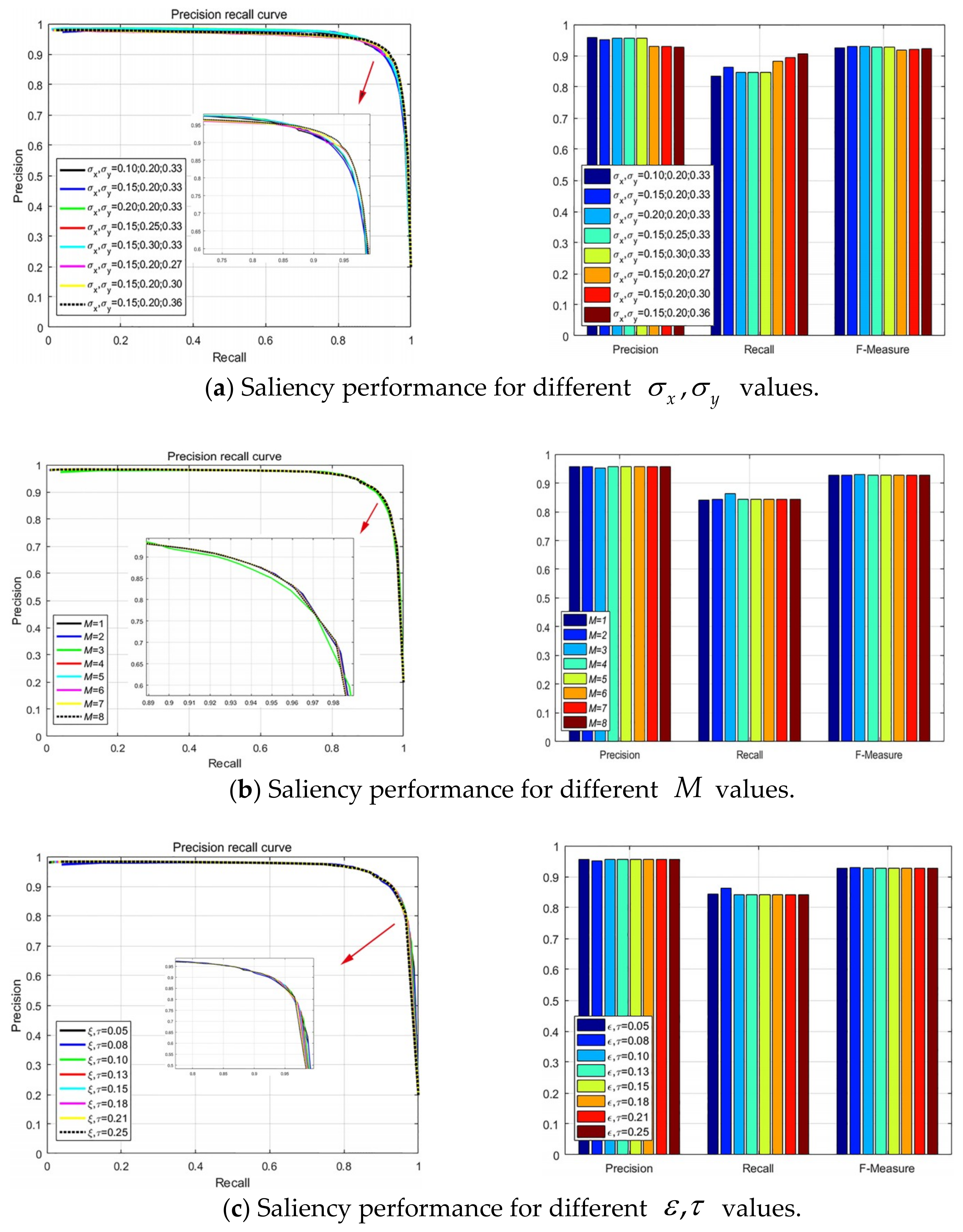
3.3. Parameter Analysis

We conducted a series of experiments to investigate the influence of various factors on saliency detection. These factors or parameters include ${\sigma }_x, {\sigma }_y$ in Equations (10), (20), and (25); the updating time $M$ in Equation (28); and the updating weight $\epsilon ,\tau$ in Equations (28) and (29); the graph with the nonlocal connections; and the integration of the feature-bias Gaussian model; the diffusion process with nonlocal connections; the single-layer updating and the multi-layer integration process. These experiments are processed in ASD dataset.

(1) Parameters: The parameter ${\sigma }_x,{\sigma }_y$ decide the distribution amplitude of Gaussian model. To precisely refine the saliency map based on different cue, the ${\sigma }_x,{\sigma }_y$ in Equations (10), (20), and (25) should be different with each other. Compactness cue denotes the spatial variance of features, but the background may be wrongly highlighted, especially when the background also has a compact distribution. So the ${\sigma }_x,{\sigma }_y$ in Equation (10) should be lower than others. Figure 9a shows the precision-recall curves and the average precisions, recalls and F-measures using an adaptive threshold with different ${\sigma }_x,{\sigma }_y$ values in Equations (10), (20), (25). As we can see, the different values of ${\sigma }_x({\sigma }_y)$ within the scope of the stated ranges have a similar result. Similarly, when the value of $M$ and $\epsilon ,\tau$ are varied, the performances change a small amount, which can be seen in Figure 9b,c. This means the performances are not sensitive to these two parameters. But to promote the recall and balance the performance, we set $M=3$ and $\epsilon =\tau =0.08$.

(2) Graph Construction: We expanded the nonlocal connections to 2-layer sparse graph. To validate it, we compared the performances of 2-layer neighborhood graph, 2-layer neighborhood graph with nonlocal connections, 2-layer sparse graph, and our proposed graph. Figure 10 shows the precision-recall curves and the average precisions, recalls and F-measures using an adaptive threshold. As is illustrated in Figure 10, the nonlocal connections can effectively promote the performance of the 2-layer neighborhood graph. Additionally, the result of the 2-layer sparse graph also has an improvement, whereas the progress may be slightly lower than 2-layer neighborhood graph. Respectively, the 2-layer sparse graph and the nonlocal connections can improve the topotaxy between different elements locally and globally. Generally, the local topotaxy may have a bigger impact of the results than the nonlocal topotaxy because of the closer spatial proximity. So as shown in Figure 10, the improvement of results via 2-layer sparse graph can be more obvious than the nonlocal connections. But the nonlocal connections can still improve the result of the 2-layer sparse graph by reducing the impact of the imprecise local connections.

(3) Component Analysis: We combined the saliency-biased Gaussian model, the diffusion process with nonlocal connections, the single-layer updating and multi-layer integration process in our algorithm. To prove the efficiency of these components, a series of experiments were carried out. The precision-recall curves and the average precisions, recalls, and F-measures at an adaptive threshold are displayed in Figure 11. As is illustrated in Figure 11b, the saliency-biased Gaussian model is effective in the improvement of precision, while the diffusion process with nonlocal connections mainly contributes to the recall. This can be explained logically. The saliency-biased Gaussian model can highlight the salient regions and compress the background, which means the high precision according to the Equation (31). Relatively, as the above mentioned, the diffusion process with nonlocal connections can obtain a more homogenous salient region, which leads to the high recall according to the Equation (32). To have a better comprehensive performance, the single-layer updating and multi-layer integration process were implemented to balance the precision and the recall.

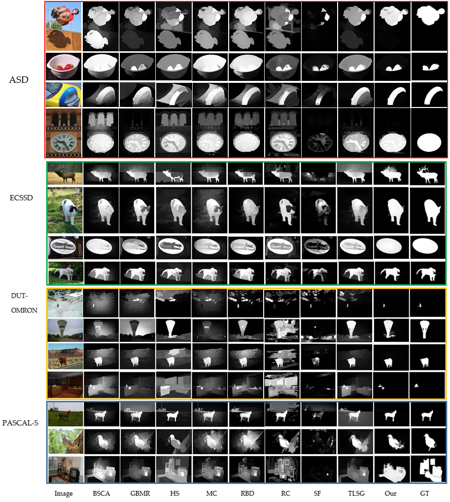
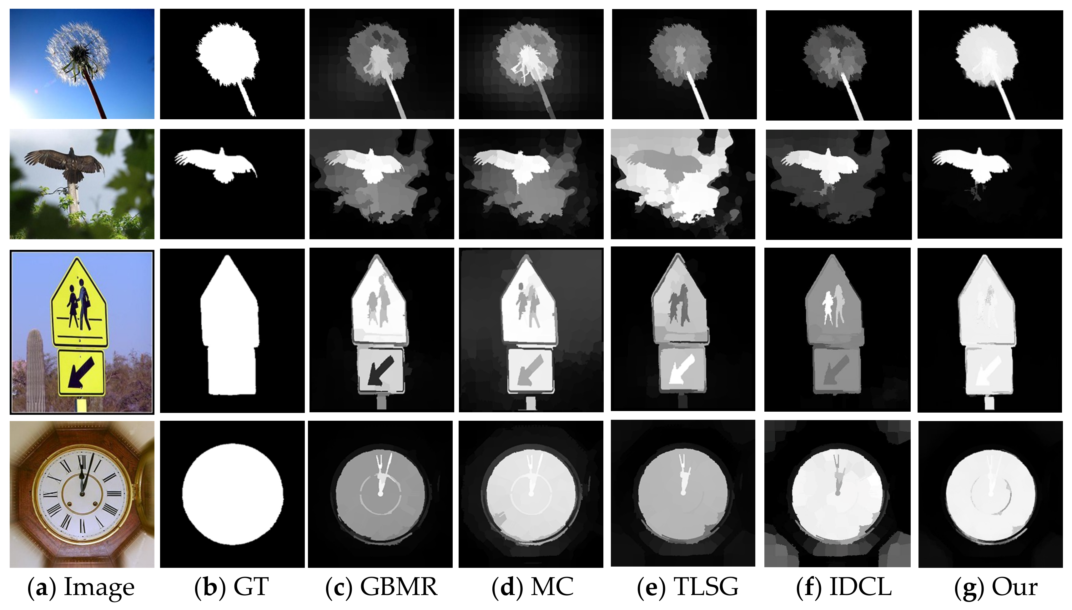
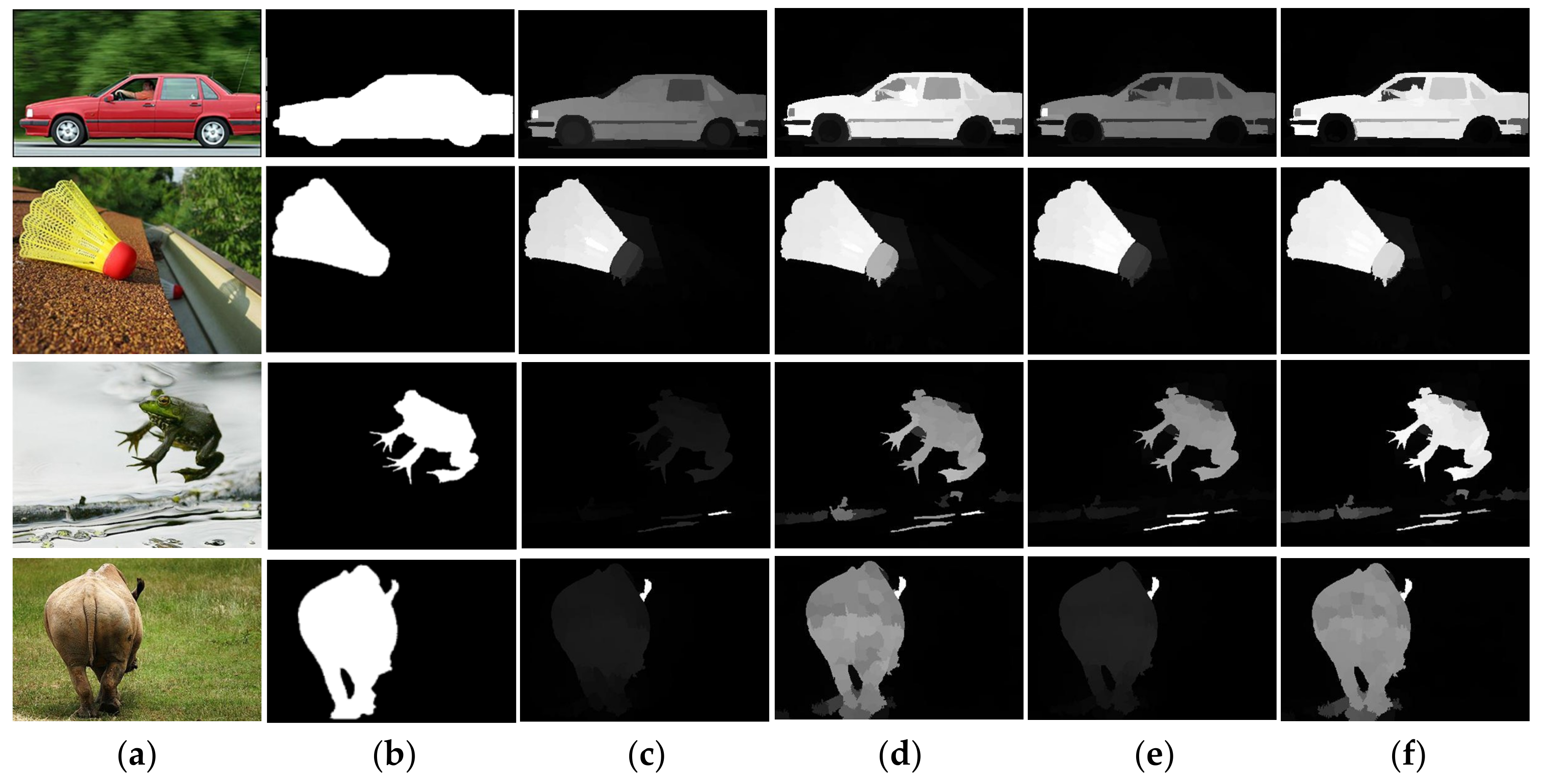
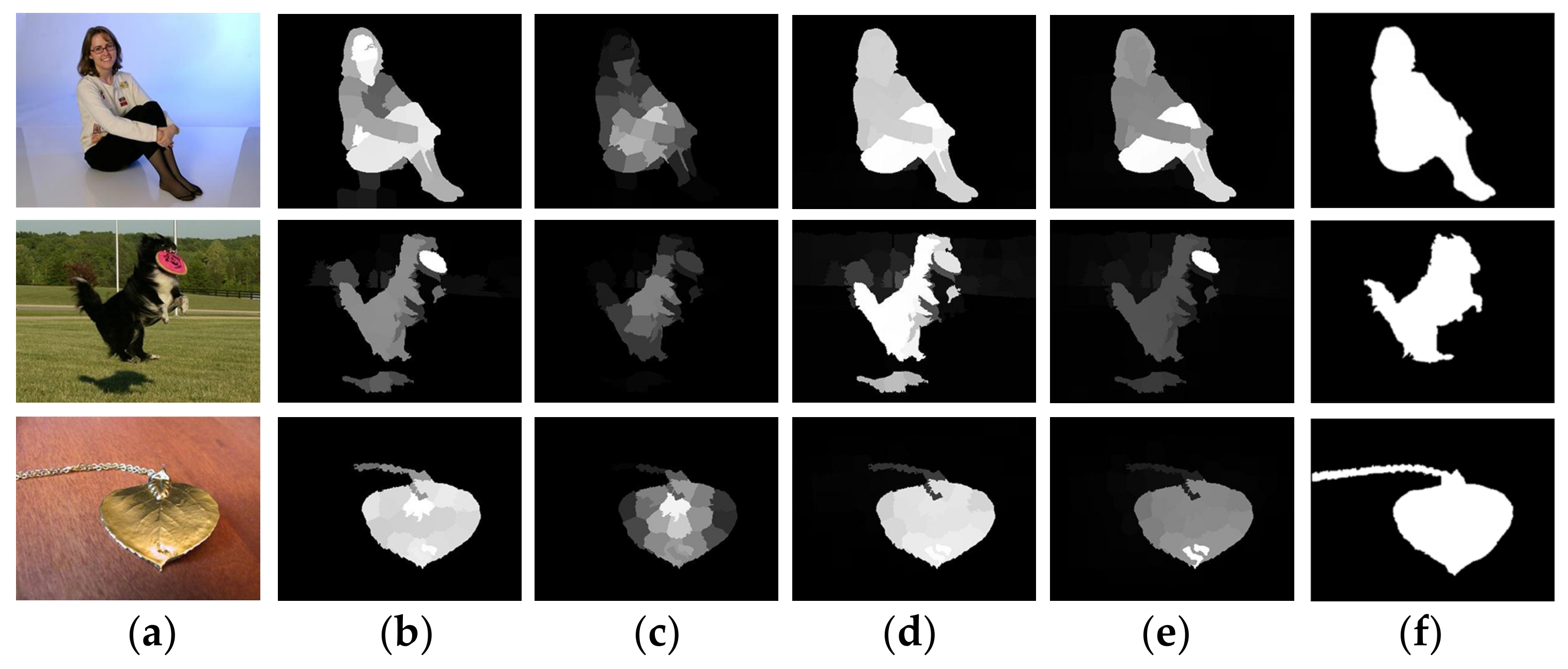
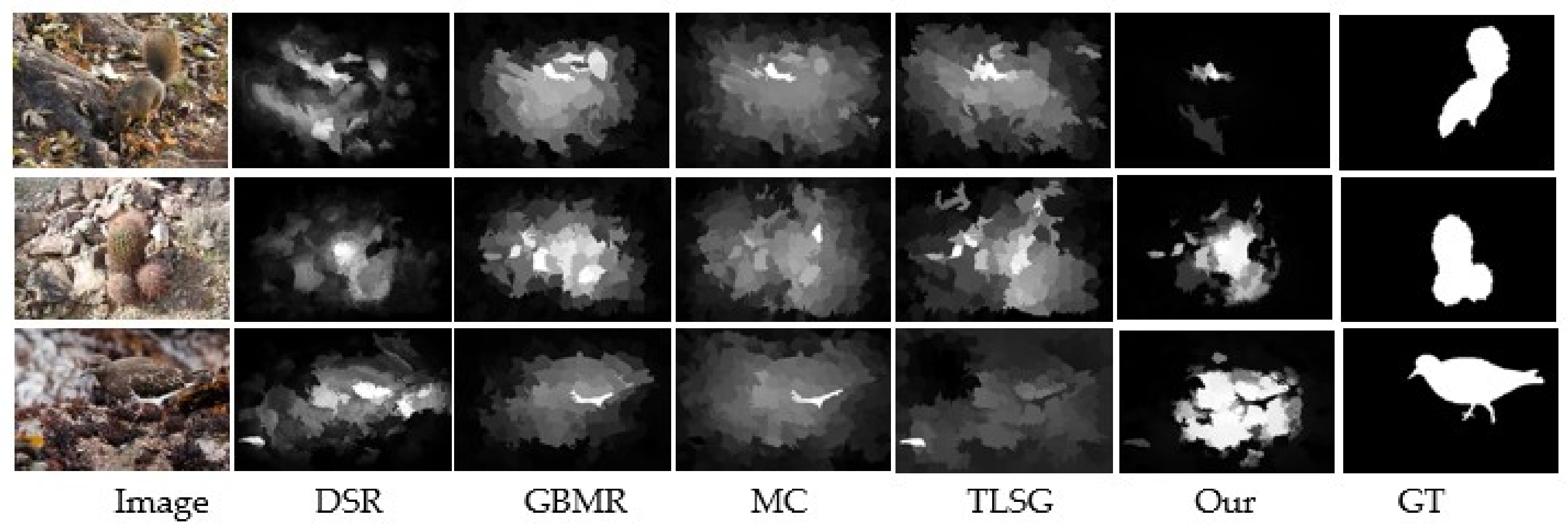
3.4. Visual Comparisons

To demonstrate the advantage of our proposed algorithm, some images with complex backgrounds are shown in Figure 12. We compared our method with state-of-the-art approaches on the ASD, ECSSD, DUT-OMRON, PASCAL-S datasets.

As Figure 12 shows, the most salient region detection methods can effectively manage cases with relatively simple backgrounds and homogenous objects. However, these methods fail to manage the complicated cases, especially when the salient object and the background are similar with each other. In contrast, our method can deal with these intricate scenarios more effectively. We compare these methods in the following two aspects: (1) the effectiveness of the background suppression; (2) the integrity and uniformity of the salient objects. First, as shown in Figure 12, only one low level cue cannot effectively suppress the background regions, such as the global contrast-based method RC [7], which can be proved with the second image in DUT-OMRON dataset. When the salient regions are compacted, SF [8] which utilizes the compactness cue can have a good performance, such as the fourth image in ASD dataset. However, SF may wrongly suppress the salient regions. In addition, the background-based method RBD [11] cannot always suppress the background effectively, such as the third image in DUT-OMRON dataset and the second image in PASCAL-S dataset. TLSG [16] which generated the saliency map with the compactness cue and diffused the saliency map on 2-layer sparse graph can obviously improve the performance in some cases, such as the second and third images in DUT-OMRON dataset. However, there still exists some cases that it cannot manage effectively, such as the first images in ECSSD dataset and PASCAL-S dataset. HS [41] which exploited the hierarchical saliency can obtain a good performance, especially when the salient objects are small, such as the second image in ASD dataset. But it cannot well suppress the background regions, such as the third images in DUT-OMRON dataset. Relatively, the diffusion-based methods BSCA [30], GBMR [23], MC [24] can obtain a homogeneous salient region. But when the salient objects are heterogeneous and the background regions are cluttered, they cannot always highlight the salient objects completely and uniformly, in some cases, they even wrongly highlight the background regions, such as the second images in ASD dataset and DUT-OMRON dataset. However, our method can manage these complicated scenarios effectively. Especially, when the salient objects are not compacted, our method can also highlight the salient region uniformly but slightly incompletely, such as the third images in the PASCAL-S dataset. What is more, our method shows the well robustness to the scale variations of the salient objects. When the salient objects are relatively small, our method can still have a good performance, which can be seen in the first and fourth images in DUT-OMRON dataset. In some scenes, the saliency maps generated by our method can almost be the same with the ground truth.

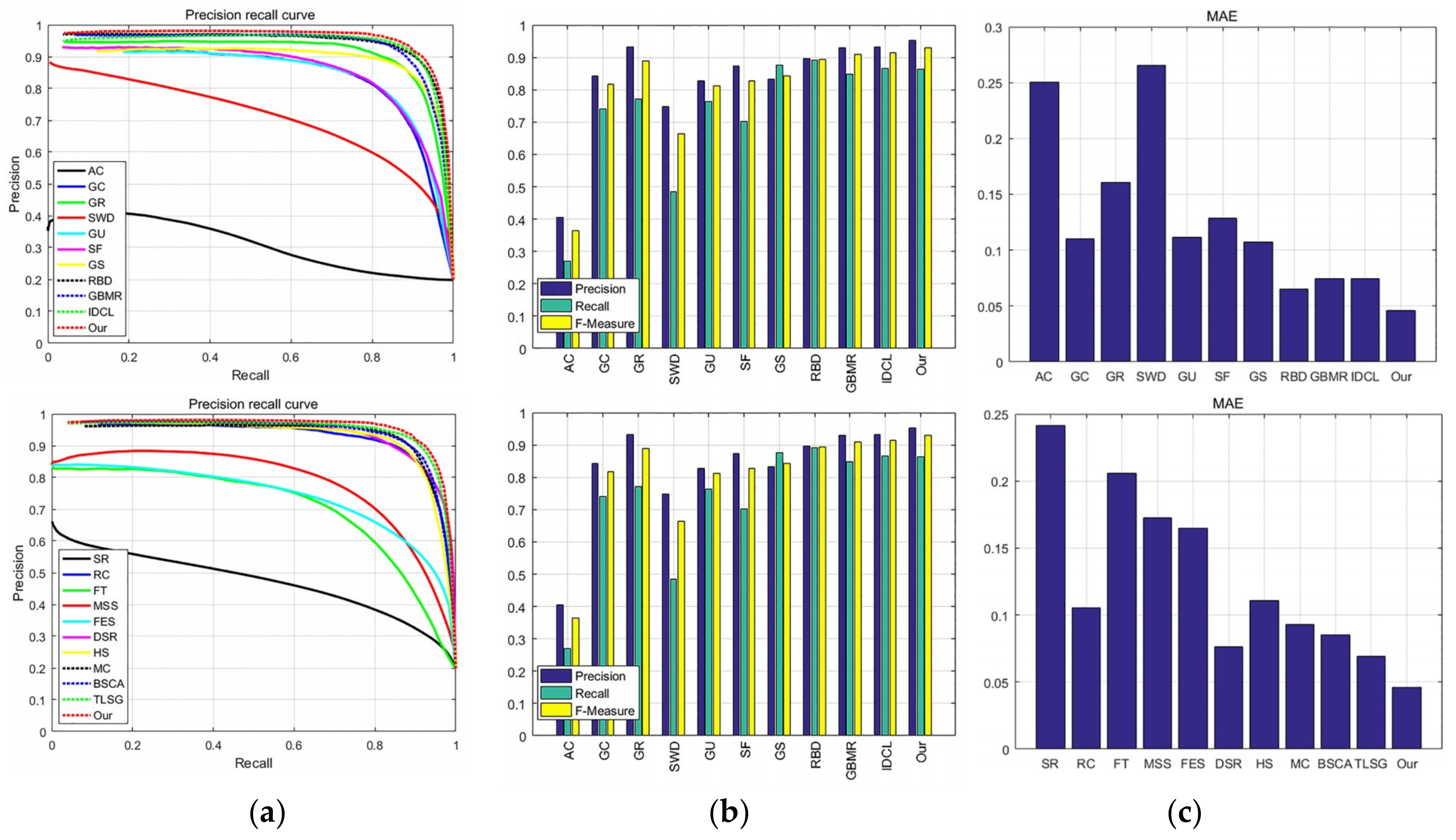
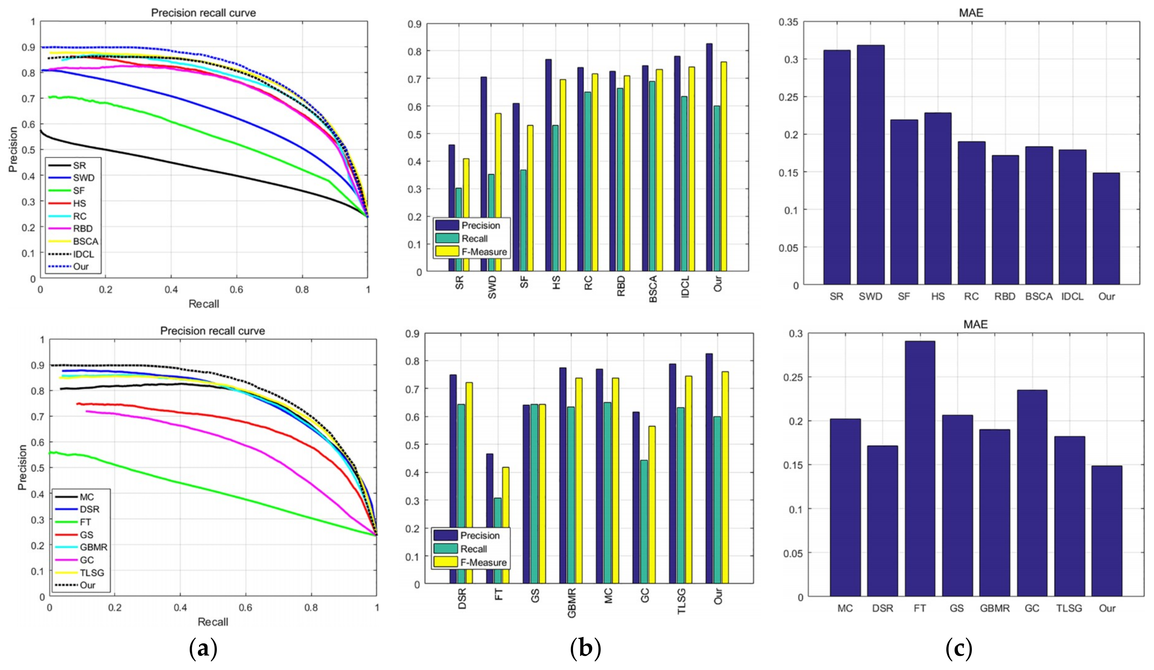
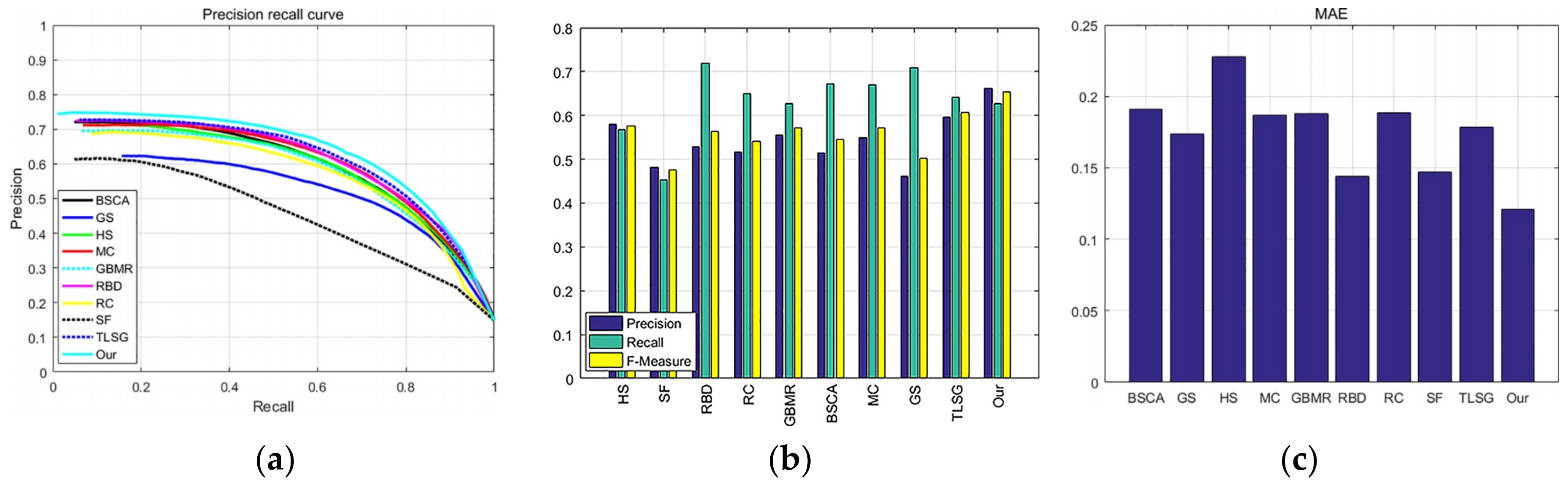
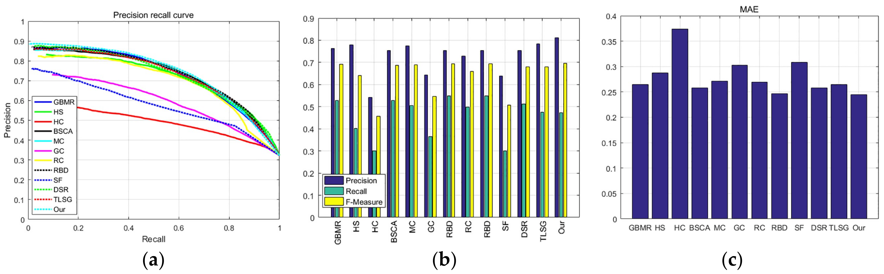
3.5. Quantitative Comparison

We quantitatively evaluated the performance of our method comparing to other published results. We carried out the experiment on the ASD, ECSSD, DUT-OMRON, and PASCAL-S datasets and compared the results using three evaluation criteria: the average precision-recall curve, F-measure, and MAE.

3.5.1. ASD

We quantitatively compared the performances of our method with 20 state-of-the-art methods: SR [13], AC [14], RC [7], FT [15], GS [10], RBD [11], DSR [12], SF [8], HS [41], GBMR [23], BSCA [30], MC [24], IDCL [9], TLSG [16], GC [43], GR [44], SWD [39], GU [43], MSS [45], and FES [46]. The performances of MC [24], GBMR [23], and RBD [11] methods are at top in a recent saliency benchmark study [47].

The average precision-recall curves in Figure 13a show the proposed method performs better than other approaches for the ASD dataset. As shown in Figure 13b, compared to the diffusion-based methods GBMR [23], BSCA [30], MC [24], IDCL [9], TLSG [16], our method can obtain a higher precision and F-measure but a slightly lower recall. In addition, the MAE of our method is lowest in these methods, which means the tiny difference between the saliency map and the ground truth.

3.5.2. ECSSD

We compared our method with 15 saliency detection algorithms: SR [13], RC [7], FT [15], GS [10], RBD [11], DSR [12], SF [8], HS [41], GBMR [23], MC [24], BSCA [30], IDCL [9], SWD [39], GC [43], and TLSG [16]. Figure 14 shows the effectiveness of our method.

The precision-recall curves in Figure 14a show the proposed approach can obtain a better performance than other methods for recall values from 0 to 0.9, but it performs poorly compared with the BSCA [30], DSR [12], and TLSG [16] for recall values from 0.9 to 1. In addition, our method can obtain a highest precision and F-measure among these saliency detection methods, which can been seen in Figure 14b. Similar with the performance of our method on ASD dataset, MAE of our method is also the lowest.

3.5.3. DUT-OMRON

Using the DUT-OMRON datasets, we quantitatively compared the proposed method with nine state-of-the-art approaches: SF [8], MC [24], RC [7], GS [10], RBD [11], HS [41], GBMR [23], BSCA [30], and TLSG [16]. As shown in Figure 15a, our method performs better than other methods for recall values from 0 to 0.95, but the precision of the proposed method is slightly lower than RBD [11] for recall values from 0.95 to 1. As Figure 15b shows, our method can obtain a highest precision and F-measure but a slightly lower recall. In addition, our method can obtain the lowest MAE, which is illustrated in Figure 15c.

3.5.4. PASCAL-S

Similarly, using the PASCAL-S datasets, we carried out the experiments to compare the proposed method with 11 approaches: RC [7], HC [7], RBD [11], SF [8], HS [41], GBMR [23], BSCA [30], TLSG [16], DSR [12], MC [24], GC [43]. The precision-recall curve in Figure 16a shows the proposed method can obtain a better performance than other methods for recall values from 0 to 0.75. Figure 16b shows the proposed method can acquire a good comprehensive performance with the highest precision and F-measure. In addition, as is illustrated in Figure 16c, these methods can obtain a similar MAE value, but the MAE of the proposed method is still lowest.

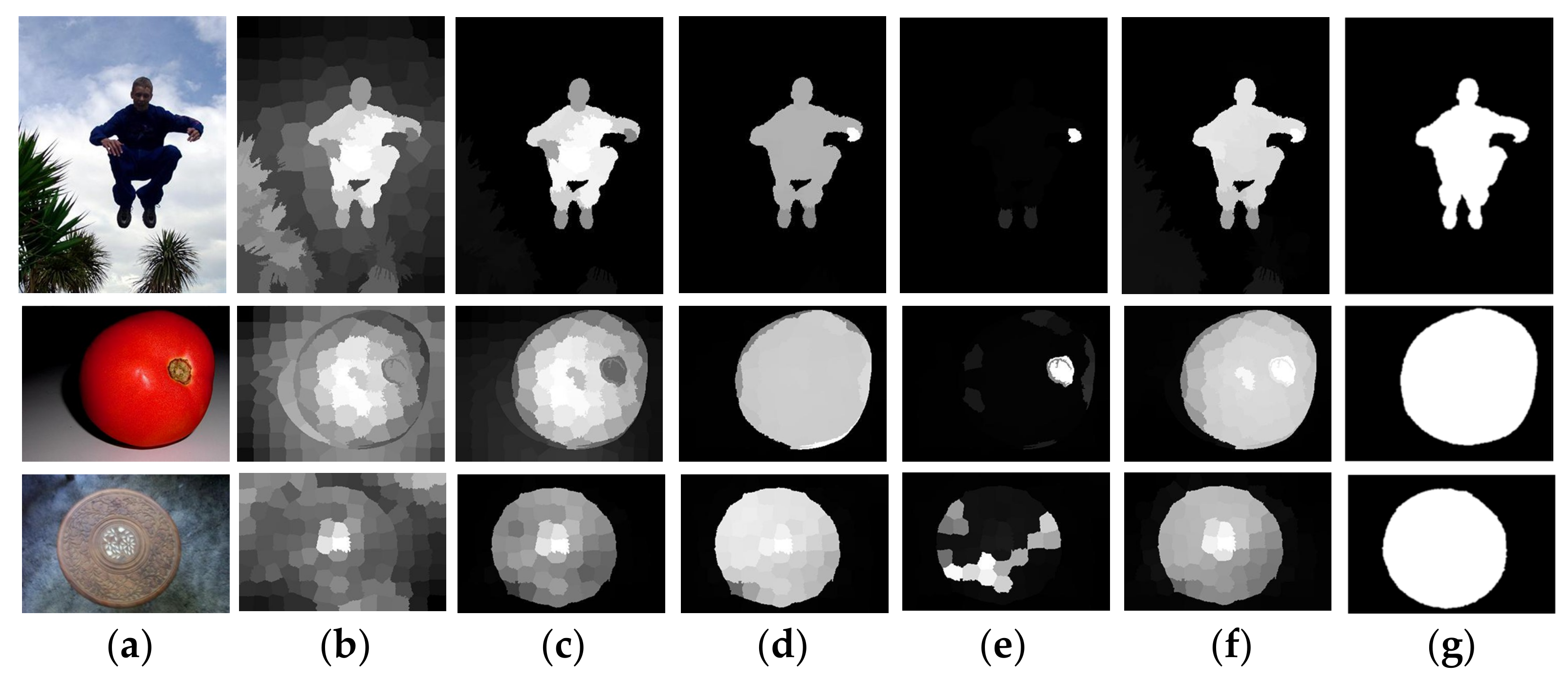
4. Failure Cases

As proved in the above section, our method performs better than most of the state-of-the-art method in term of various evaluation metrics. However, the proposed method mainly depends on the color information: the compactness cue considers the spatial variance of the color, while the uniqueness cue uses the color contrast in the color space. Therefore, it may fail to manage the images that do not have much color variation, especially when foreground and background objects have similar colors. Figure 17 shows the estimated salient region produced by our method is inaccurate. To overcome this limitation, some studies have been conducted by incorporating more features such as texture [48] or even high-level knowledge [49]. We will work on these problems in the future.

5. Conclusions

In this paper, we proposed a saliency detection method by propagating the saliency seed vectors calculated via compactness and uniqueness cues. First, we obtained the initial saliency maps based on the optimized compactness and uniqueness cues. Then, a saliency-biased Gaussian model was designed to refine the saliency maps more precisely. After considering the limitation of the local intrinsic relevance, we exploited the nonlocal intrinsic relevance into 2-layer sparse graph to obtain a more homogeneous salient region. Finally, we presented a single-layer updating and multi-layer integration algorithm to effectively excavate the multi-scale saliency information. The comprehensive experimental results demonstrated the effectiveness of the proposed method. What is more, the salient regions generated by our method are uniform and highlighted, which is significant for the subsequent image operations, such as object segmentation and object classification.

References

- Chang, K.Y.; Liu, T.L.; Lai, S.H. From co-saliency to co-segmentation: An efficient and fully unsupervised energy minimization model. In Proceedings of the IEEE Conference on Computer Vision and Pattern Recognition, Colorado Springs, CO, USA, 20–25 June 2011; pp. 2129–2136. [Google Scholar]
- Alexe, B.; Deselaers, T.; Ferrari, V. Measuring the Objectness of Image Windows. IEEE Trans. Pattern Anal. Mach. Intell. 2012, 34, 2189–2202. [Google Scholar] [CrossRef] [PubMed] [Green Version]
- Walther, D.; Rutishauser, U.; Koch, C.; Perona, P. Selective visual attention enables learning and recognition of multiple objects in cluttered scenes. Comput. Vis. Image Underst. 2005, 100, 41–63. [Google Scholar] [CrossRef] [Green Version]
- Guo, C.; Zhang, L. A novel multiresolution spatiotemporal saliency detection model and its applications in image and video compression. Oncogene 1988, 3, 523. [Google Scholar]
- Alexe, B.; Deselaers, T.; Ferrari, V. What is an object? In Proceedings of the Computer Vision and Pattern Recognition, Columbus, OH, USA, 23–28 June 2014; pp. 73–80. [Google Scholar]
- Yang, J.; Yang, M.H. Top-down visual saliency via joint CRF and dictionary learning. In Proceedings of the Computer Vision and Pattern Recognition, Providence, RI, USA, 16–21 June 2012; pp. 2296–2303. [Google Scholar]
- Cheng, M.M.; Zhang, G.X.; Mitra, N.J.; Huang, X. Global contrast based salient region detection. In Proceedings of the Computer Vision and Pattern Recognition, Colorado Springs, CO, USA, 20–25 June 2011; pp. 409–416. [Google Scholar]
- Hornung, A.; Pritch, Y.; Krahenbuhl, P.; Perazzi, F. Saliency filters: Contrast based filtering for salient region detection. In Proceedings of the IEEE Conference on Computer Vision and Pattern Recognition, Providence, RI, USA, 16–21 June 2012; pp. 733–740. [Google Scholar]
- Zhou, L.; Yang, Z.; Yuan, Q.; Zhou, Z.; Hu, D. Salient Region Detection via Integrating Diffusion-Based Compactness and Local Contrast. IEEE Trans. Image Process. 2015, 24, 3308–3320. [Google Scholar] [CrossRef] [PubMed]
- Wei, Y.; Wen, F.; Zhu, W.; Sun, J. Geodesic Saliency Using Background Priors. In Proceedings of the European Conference on Computer Vision, Florence, Italy, 7–13 October 2012; pp. 29–42. [Google Scholar]
- Zhu, W.; Liang, S.; Wei, Y.; Sun, J. Saliency Optimization from Robust Background Detection. In Proceedings of the IEEE Conference on Computer Vision and Pattern Recognition, Columbus, OH, USA, 23–28 June 2014; pp. 2814–2821. [Google Scholar]
- Li, X.; Lu, H.; Zhang, L.; Xiang, R.; Yang, M.H. Saliency Detection via Dense and Sparse Reconstruction. In Proceedings of the IEEE International Conference on Computer Vision, Sydney, Australia, 1–8 December 2013; pp. 2976–2983. [Google Scholar]
- Hou, X.; Zhang, L. Saliency Detection: A Spectral Residual Approach. In Proceedings of the IEEE Conference on Computer Vision and Pattern Recognition, Minneapolis, MN, USA, 18–23 June 2007; pp. 1–8. [Google Scholar]
- Achanta, R.; Estrada, F.; Wils, P.; Sstrunk, S. Salient region detection and segmentation. ICVS 2008, 5008, 66–75. [Google Scholar]
- Achanta, R.; Hemami, S.; Estrada, F.; Susstrunk, S. Frequency-tuned salient region detection. In Proceedings of the IEEE Conference on Computer Vision and Pattern Recognition, CVPR 2009, Miami, FL, USA, 20–25 June 2009; pp. 1597–1604. [Google Scholar]
- Zhou, L.; Yang, Z.; Zhou, Z.; Hu, D. Salient Region Detection using Diffusion Process on a 2-Layer Sparse Graph. IEEE Trans Image Process. 2017, 26, 5882–5894. [Google Scholar] [CrossRef] [PubMed]
- Schölkopf, B.; Platt, J.; Hofmann, T. Graph-Based Visual Saliency. Proc Neural Inf. Process. Syst. 2006, 19, 545–552. [Google Scholar]
- Liu, T.; Sun, J.; Zheng, N.N.; Tang, X.; Shum, H.Y. Learning to Detect A Salient Object. In Proceedings of the IEEE Conference on Computer Vision and Pattern Recognition, Minneapolis, MN, USA, 17–22 June 2007; pp. 1–8. [Google Scholar]
- Chang, K.Y.; Liu, T.L.; Chen, H.T.; Lai, S.H. Fusing generic objectness and visual saliency for salient object detection. In Proceedings of the International Conference on Computer Vision, Barcelona, Spain, 6–13 November 2011; pp. 914–921. [Google Scholar]
- Ren, Z.; Hu, Y.; Chia, L.T.; Rajan, D. Improved saliency detection based on superpixel clustering and saliency propagation. In Proceedings of the ACM International Conference on Multimedia, Firenze, Italy, 25–29 October 2010; pp. 1099–1102. [Google Scholar]
- Mai, L.; Niu, Y.; Liu, F. Saliency Aggregation: A Data-Driven Approach. In Proceedings of the IEEE Conference on Computer Vision and Pattern Recognition, Portland, OR, USA, 23–28 June 2013; pp. 1131–1138. [Google Scholar]
- Gopalakrishnan, V.; Hu, Y.; Rajan, D. Random walks on graphs for salient object detection in images. IEEE Trans Image Process. 2010, 19, 3232–3242. [Google Scholar] [CrossRef] [PubMed]
- Yang, C.; Zhang, L.; Lu, H.; Xiang, R.; Yang, M.H. Saliency Detection via Graph-Based Manifold Ranking. In Proceedings of the IEEE Conference on Computer Vision and Pattern Recognition, Portland, OR, USA, 23–28 June 2013; pp. 3166–3173. [Google Scholar]
- Jiang, B.; Zhang, L.; Lu, H.; Yang, C.; Yang, M.-H. Saliency Detection via Absorbing Markov Chain. IEEE Int. Conf. Comput. Vis. 2013. [Google Scholar] [CrossRef] [Green Version]
- Zhang, L.; Ai, J.; Jiang, B.; Lu, H.; Li, X. Saliency Detection via Absorbing Markov Chain with Learnt Transition Probability. In Proceedings of the IEEE International Conference on Computer Vision, Sydney, Australia, 1–8 December 2013; pp. 1665–1672. [Google Scholar]
- Lu, S.; Mahadevan, V.; Vasconcelos, N. Learning Optimal Seeds for Diffusion-Based Salient Object Detection. In Proceedings of the Computer Vision and Pattern Recognition, Columbus, OH, USA, 23–28 June 2014; pp. 2790–2797. [Google Scholar]
- Sun, J.; Lu, H.; Liu, X. Saliency Region Detection Based on Markov Absorption Probabilities. IEEE Trans. Image Process. 2015, 24, 1639–1649. [Google Scholar] [CrossRef] [PubMed]
- Jiang, P.; Vasconcelos, N.; Peng, J. Generic Promotion of Diffusion-Based Salient Object Detection. In Proceedings of the IEEE International Conference on Computer Vision, Santiago, Chile, 7–13 December 2015; pp. 217–225. [Google Scholar]
- Li, C.; Yuan, Y.; Cai, W.; Xia, Y. Robust saliency detection via regularized random walks ranking. In Proceedings of the 2015 IEEE Conference on Computer Vision and Pattern Recognition (CVPR) (2015), Boston, MA, USA, 7–12 June 2015; pp. 2710–2717. [Google Scholar]
- Qin, Y.; Lu, H.; Xu, Y.; Wang, H. Saliency detection via Cellular Automata. In Proceedings of the Computer Vision and Pattern Recognition, Boston, MA, USA, 7–12 June 2015; pp. 110–119. [Google Scholar]
- Li, H.; Lu, H.; Lin, Z.; Shen, X.; Price, B. Inner and inter label propagation: Salient object detection in the wild. IEEE Trans Image Process. 2015, 24, 3176–3186. [Google Scholar] [CrossRef] [PubMed]
- Gong, C.; Tao, D.; Liu, W.; Maybank, S.J.; Fang, M.; Fu, K.; Yang, J. Saliency propagation from simple to difficult. In Proceedings of the IEEE Conference on Computer Vision and Pattern Recognition, Boston, MA, USA, 7–12 June 2015; pp. 2531–2539. [Google Scholar]
- Qiu, Y.; Sun, X.; She, M.F. Saliency detection using hierarchical manifold learning. Neurocomputing 2015, 168, 538–549. [Google Scholar] [CrossRef]
- Xiang, D.; Wang, Z. Salient Object Detection via Saliency Spread; Springer International Publishing: New York, NY, USA, 2014; pp. 457–472. [Google Scholar]
- Zhou, L.; Yang, S.; Yang, Y.; Yang, Z. Geodesic distance and compactness prior based salient region detection. In Proceedings of the International Conference on Image and Vision Computing, Palmerston North, New Zealand, 21–22 November 2016; pp. 1–5. [Google Scholar]
- Wang, Z.; Xiang, D.; Hou, S.; Wu, F. Background-Driven Salient Object Detection. IEEE Trans. Multimedia 2017. [Google Scholar] [CrossRef]
- Achanta, R.; Shaji, A.; Smith, K.; Lucchi, A.; Fua, P.; Süsstrunk, S. SLIC Superpixels Compared to State-of-the-Art Superpixel Methods. IEEE Trans. Pattern Anal. Mach. Intell. 2012, 34, 2274–2282. [Google Scholar] [CrossRef] [PubMed] [Green Version]
- Shen, X.; Wu, Y. A unified approach to salient object detection via low rank matrix recovery. In Proceedings of the IEEE Conference on Computer Vision and Pattern Recognition, Providence, RI, USA, 16–21 June 2012; pp. 853–860. [Google Scholar]
- Duan, L.; Wu, C.; Miao, J.; Qing, L.; Fu, Y. Visual saliency detection by spatially weighted dissimilarity. In Proceedings of the Computer Vision and Pattern Recognition, Colorado Springs, CO, USA, 20–25 June 2011; pp. 473–480. [Google Scholar]
- Otsu, N. Threshold Selection Method from Gray-Level Histograms. IEEE Trans. Syst. Man Cybern. 1979, 9, 62–66. [Google Scholar] [CrossRef]
- Yan, Q.; Xu, L.; Shi, J.; Jia, J. Hierarchical Saliency Detection. In Proceedings of the Computer Vision and Pattern Recognition, Portland, OR, USA, 23–28 June 2013; pp. 1155–1162. [Google Scholar]
- Li, Y.; Hou, X.; Koch, C.; Rehg, J.M.; Yuille, A.L. The Secrets of Salient Object Segmentation. In Proceedings of the Computer Vision and Pattern Recognition, Columbus, OH, USA, 23–28 June 2014; pp. 280–287. [Google Scholar]
- Cheng, M.M.; Warrell, J.; Lin, W.Y.; Zheng, S.; Vineet, V.; Crook, N. Efficient Salient Region Detection with Soft Image Abstraction. In Proceedings of the IEEE International Conference on Computer Vision, Sydney, Australia, 1–8 December 2013; pp. 1529–1536. [Google Scholar]
- Yang, C.; Zhang, L.; Lu, H. Graph-Regularized Saliency Detection With Convex-Hull-Based Center Prior. IEEE Signal Process. Lett. 2013, 20, 637–640. [Google Scholar] [CrossRef]
- Achanta, R.; Süsstrunk, S. Saliency detection using maximum symmetric surround. In Proceedings of the IEEE International Conference on Image Processing, Hong Kong, China, 26–29 September 2010; pp. 2653–2656. [Google Scholar]
- Tavakoli, H.R.; Rahtu, E. Fast and efficient saliency detection using sparse sampling and kernel density estimation. In Proceedings of the Scandinavian Conference on Image Analysis, Ystad, Sweden, 23–27 May 2011; pp. 666–675. [Google Scholar]
- Borji, A.; Cheng, M.M.; Jiang, H.; Li, J. Salient Object Detection: A Benchmark. IEEE Trans. Image Process. 2015, 24, 5706–5722. [Google Scholar] [CrossRef] [Green Version]
- Shuai, J.; Qing, L.; Miao, J.; Ma, Z.; Chen, X. Salient region detection via texture-suppressed background contrast. In Proceedings of the IEEE International Conference on Image Processing, Melbourne, Australia, 15–18 September 2013; pp. 2470–2474. [Google Scholar]
- Yan, X.; Wang, Y.; Song, Q.; Dai, K. Salient object detection via boosting object-level distinctiveness and saliency refinement. J. Vis. Commun. Image Represent. 2017. [Google Scholar] [CrossRef]
© 2018 by the authors. Licensee MDPI, Basel, Switzerland. This article is an open access article distributed under the terms and conditions of the Creative Commons Attribution (CC BY) license (http://creativecommons.org/licenses/by/4.0/).
Share and Cite
Luo, H.; Han, G.; Liu, P.; Wu, Y. Salient Region Detection Using Diffusion Process with Nonlocal Connections. Appl. Sci. 2018, 8, 2526. https://doi.org/10.3390/app8122526
Luo H, Han G, Liu P, Wu Y. Salient Region Detection Using Diffusion Process with Nonlocal Connections. Applied Sciences. 2018; 8(12):2526. https://doi.org/10.3390/app8122526
Chicago/Turabian StyleLuo, Huiyuan, Guangliang Han, Peixun Liu, and Yanfeng Wu. 2018. "Salient Region Detection Using Diffusion Process with Nonlocal Connections" Applied Sciences 8, no. 12: 2526. https://doi.org/10.3390/app8122526
APA StyleLuo, H., Han, G., Liu, P., & Wu, Y. (2018). Salient Region Detection Using Diffusion Process with Nonlocal Connections. Applied Sciences, 8(12), 2526. https://doi.org/10.3390/app8122526