Article

Three Dimensional CS-FEM Phase-Field Modeling Technique for Brittle Fracture in Elastic Solids

Department of Aerospace Engineering and Engineering Mechanics, University of Cincinnati, Cincinnati, OH 45219, USA
*
Author to whom correspondence should be addressed.
Appl. Sci. 2018, 8(12), 2488; https://doi.org/10.3390/app8122488
Submission received: 30 October 2018 / Revised: 22 November 2018 / Accepted: 22 November 2018 / Published: 4 December 2018
(This article belongs to the Special Issue Computational Methods for Fracture)

Abstract

:
The cell based smoothed finite element method (CS-FEM) was integrated with the phase-field technique to model brittle fracture in 3D elastic solids. The CS-FEM was used to model the mechanics behavior and the phase-field method was used for diffuse fracture modeling technique where the damage in a system was quantified by a scalar variable. The integrated CS-FEM phase-field approach provides an efficient technique to model complex crack topologies in three dimensions. The detailed formulation of our combined method is provided. It was implemented in the commercial software ABAQUS using its user-element (UEL) and user-material (UMAT) subroutines. The coupled system of equations were solved in a staggered fashion using the in-built non-linear Newton–Raphson solver in ABAQUS. Eight node hexahedral (H8) elements with eight smoothing domains were coded in CS-FEM. Several representative numerical examples are presented to demonstrate the capability of the method. We also discuss some of its limitations.

1. Introduction

In the past decade, Liu et al. [1,2] generalized the gradient smoothing approach in meshfree method [3] and proposed the smoothed finite element method(S-FEM) to overcome some of the inherent shortcomings of the classical finite element method(FEM) such as overly stiff behavior, sensitivity to mesh distortions, and stress inaccuracy. The SFEM combines the FEM with the traditional meshfree methods in producing more accurate results with higher efficiency [1,2]. It uses the base mesh of the FEM and reconstructs the strain field using the gradient smoothing technique. Thus, in contrast to the weak formulations of the FEM [4], the weakened weak formulation used here [1,2] further softens the model [5], giving it a closer to exact stiffness [6]. The gradient smoothing operation facilitates creation of various smoothing domains based on elements, nodes, edges (2D), and faces (3D) over which the stress/strain is evaluated [1]. This, in turn, produces a wide variety of results and gives the analyst much needed freedom to design models as per the requirement. For example, the node based smoothing domains (NS-FEM) produce upper bound solutions for force driven problems [7]. The edge/face based smoothing domains (ES/FS-FEM) produce very accurate results using even triangular and tetrahedral mesh [8]. A combination of the NS-FEM and the ES-FEM produces very accurate close to exact solutions in the error norm [6,9]. Amongst other applications [10,11,12,13,14], the S-FEM has been effectively applied to fracture problems for quasi-static crack propagation [15], anisotropic materials [16], dynamic fracture [1] and for singular geometries of arbitrary order [17,18]. Although these studies have proven to be quite accurate and efficient when compared to the FEM, they treat the crack as an discrete entity, a formulation which has its own inherent problems.
Fracture is the primary cause of failure in the majority of engineering structures. An initially existing small crack often leads to catastrophic failures by propagation under external loads. Over the past few decades, several theories and computational techniques have been developed to accurately model fracture and predict crack propagation in engineering systems. Classically, cracks are dealt with discretely in theoretical/computational fracture mechanics. The discontinuities have been separately modeled and special methodologies have been developed to accurately model the singular stress field near the crack tip. The collapsed quadrilateral or triangular element in the FEM [4] is the most widely used, however several other methods such as the boundary element method (BEM) [19], mesh-free methods [3,20], the extended finite element method [21], and SFEM [18,22,23] have proven to be equally efficient. BEM uses a mesh only on the boundaries, thereby reducing the computational complexity by one order, but is unable to treat material non-linearities. S-FEM uses a base mesh of linear elements with an enrichment only around the crack-tip, thereby mitigating the computational cost of using a quadratic mesh throughout the domain [18]. However, in S-FEM, as in the classical FEM, the crack path is mesh dependent; cracks can only propagate along edges of elements and the tracking of crack front for three-dimensional problems is computationally very expensive. The X-FEM overcomes this mesh dependency but uses additional degrees of freedom and the integration in the weak form for the elements containing the crack becomes particularly very complex in three-dimensional fracture problems.
An alternate way of modeling fracture has gained popularity in the computational community in the past decade or two. In this method, the crack is modeled as a diffused entity and represented by a continuous scalar variable called the phase-field [24]. This variable differentiates between the broken and intact material phases and, contrary to the discrete approach, provides a smooth transition between them [25,26,27,28]. This method is based on the variational theory of fracture [24] addressing the shortcomings of the original Griffith’s theory, which could not predict crack nucleation or complex crack paths. The elegance of this method lies in the fact that it can successfully predict complex crack behaviors such as crack branching, curved crack paths, and crack merging even in three dimensions without any ad-hoc criterion. This gives it an immediate advantage over the traditional methods where the prediction of such phenomenons is quite complex. Apart from the primary applications of brittle fracture [28], the phase-field approach has been developed and applied to many complex fracture mechanics problems including large deformations [29], plasticity [30], multiphysics [31,32], and dynamics [33,34]. It has also been previously implemented in the commercial code ABAQUS by using its user subroutine features [27,28]. The phase-field model, however, is not without its disadvantages, including having a very refined mesh in the expected crack propagation region. Advanced fracture algorithms such as the screened Poisson’s equations [35,36,37] for crack propagation are developed to overcome such shortcomings. However, here we limit ourselves to the application of the phase-field method and discuss its useful features as well as disadvantages.
In this work, we integrate the cell based S-FEM with phase-field model to simulate 3-D crack propagation. This integration is done on the commercial platform of ABAQUS. ABAQUS is one of the most widely used commercial codes and its excellent inbuilt solvers and sophisticated visualization tools are particularly attractive for implementing user developed element formulations. A CS-FEM formulation for the eight-node hexahedral elements (3D-CS-FEM-H8) is used, similar to the one used in Xuan et al. [38]. We consider each node to have an additional degree of freedom (phase-field) in addition to the standard displacements. The phase-field and the displacement variables are solved in a staggered fashion to attenuate instability [27]. The 3D CS-FEM-H8 has already been proven to have faster convergence rate and better accuracy than the standard FEM, thus its assimilation with the phase-field method which computes complex crack topologies without any ad-hoc criterion, produces another efficient technique to model crack propagation. One of the significant disadvantages of implementing this method in ABAQUS is that the software does not let users access data for any surrounding elements, thus we deviate from the classical way of calculating strains/stresses in CS-FEM [1,38], and develop another novel, simple yet quite effective approach. It is noteworthy that this is also the reason for our inability to implement S-FEM models of higher accuracy into the software. However, with all these shortcomings, as demonstrated by a number of examples, this method proves to be quite an effective tool to predict complex crack behaviors.
This paper is outlined as follows: In Section 2, we outline the phase-field model of fracture and the 3D-CS-FEM-H8, and discuss the implementation details of the combined method into ABAQUS. In Section 3, we provide numerical examples to validate our method. In Section 4, we conclude the paper with a summary of our findings and proposed future works.

2. Methods

2.1. Governing Equations of a 3D Elastic Solid with Discontinuity

Consider a three-dimensional (3D) arbitrary, homogeneous, linear elastic domain Ω bounded by Γ such that Γ = Γ u Γ t , Γ u Γ t = 0 and an internal traction free crack Γ c , as shown in Figure 1, where Γ u and Γ t are the displacement and traction boundary surfaces, respectively. The equilibrium equations are given as [1,4]:
· σ + f b = 0
where ∇ is the divergence operator, σ is the Cauchy stress tensor and f b is the body force.
The Dirichlet and Neumann boundary conditions are given as:
u ( x , t ) = u ¯ ( x , t ) on Γ u
σ · n = f t on Γ t
σ · n = 0 on Γ c
where n is the outward unit normal vector on the boundary area Γ and u ¯ is the prescribed displacement on the boundary Γ u .
The stress–strain relation is given by the constitutive equation
σ = C · ϵ
where C is the matrix of elastic constants.
Assuming small displacements and strain, we can define the compatibility relation between strain and displacement as:
ϵ = s u ( x )
The elastic strain energy density is given by
ψ e ( ϵ ) = 1 2 λ ϵ ii ϵ jj + μ ϵ ij ϵ ij
where λ and μ are the Lamé constants.

2.2. Review of Phase-Field Model for Brittle Fracture

Following the derivations in [25,27,39], we discuss briefly about the formulations of phase-field approximations for diffuse fracture modeling.
According to the variational theory of fracture, the crack propagates in such a way the total energy of a system is always minimized. Thus, we approach by minimizing the energy functional. The total energy of a discontinuous system is given by
Π = ψ e ( ϵ ) + ψ f ψ e x t ( u )
where ψ e ( ϵ ) is the elastic strain energy as given in Equation (7) integrated over the entire volume Ω , ψ f is the fracture surface energy and ψ e x t ( u ) is the external potential energy.
The fracture surface energy ψ f is given by
ψ f = G c Ω γ ( c ) d Ω
where G c is the critical energy release rate proposed by Griffith, c is the phase-field parameter and γ ( c ) is the density function which was calculated to be [28]
γ ( c ) = 1 2 [ 1 l c c 2 + l c 2 | c | 2 ]
where l c is the length scale parameter.
The external potential energy is given by the summation of the body force b and the surface traction t Γ :
Ψ e x t ( u ) = Ω b · u d V + Γ t Γ · u d A
The total internal potential energy of a system can be written as the summation of the bulk energy and the energy required for the formation of crack [24,28,39]
Ψ ( u , c ) = Ω [ ( 1 c ) 2 + d ] ψ ( ϵ ) d Ω + Ω G c 2 [ l c c · c + 1 l c c 2 ] d Ω
where d is a numerical stabilization parameter.
By variation of the external and internal energy potentials (using Equations (8)–(12)) and thereby imposing the principal of virtual displacements we obtain the governing equations of the model:
[ ( 1 c ) 2 + d ] σ ij x i + b j = 0 in Ω
[ ( 1 c ) 2 + d ] n i σ ij = t j in Γ t
u j = u ¯ j in Γ u
G c l c 2 c x i x i + [ G c l c + 2 ψ ( ϵ ) ] c = 2 ψ ( ϵ ) in Ω
c x i n i = 0 in Γ

2.3. Three-Dimensional Cell Based Smoothed-Finite Elements

In S-FEM, the idea of strain smoothing is combined with the standard underlying mesh of FEA by dividing each element into a number of sub-cells [1]. We use the eight-noded hexahedral elements with eight smoothing cells (Figure 2). They have already been proven to have a better accuracy than the standard eight-noded hexahedral element used in FEA with eight Gaussian points [38] using the same set of elements. Classical FEM involves isoparametric transformation for every element, making the problem very much mesh dependent because it involves inverting the Jacobian matrix. The solutions tend to vary with minor mesh distortions and for better modeling of certain topological features one needs mesh refinement or higher order elements, which makes the problem computationally expensive. The S-FEM can solve majority of computational problems using a base of linear triangular/tetrahedral mesh, which can be generated automatically. Since the shape functions are created on the basis of radial point interpolation, creating special elements to treat special topological features [18] is of minor hassle and does not need any transition or patch elements. In S-FEM, a smoothing operation is performed on the gradient of the displacement field for each smoothing cell in an element. Subsequently, the interior integration on each of the smoothing cell is transferred to the boundary surface area using the divergence theorem. Herein lies one of the biggest advantages of the S-FEM. This feature makes the solution pretty impervious to mesh distortion since we can avoid the isoparametric transformation and also contributes in saving computational cost. In this case, the gradient smoothing is the spatial average of the strain, over a smoothing hexahedral cell. A smoothing operation is performed to the gradient of displacement for each smoothing cell in an element:
u h ( x C ) = Ω u h ( x ) Φ ( x x C ) d Ω
where x C and Ω represent the center and volume of the smoothing domain, respectively, and Φ is a smoothing function.
Integration by parts on Equation (18) yields:
u h ( x C ) = Γ u h ( x ) n ( x ) Φ ( x x C ) d Γ Ω u h ( x ) Φ ( x x C ) d Ω
For simplicity, a piecewise constant smoothing function is applied, which is assumed to be constant within Ω C and vanish everywhere else,
Φ ( x x C ) = 1 V c for x Ω c 0 for x Ω c
where V C = Ω c d Ω and Ω c is the smoothing cell.
Substituting Equation (20) into Equation (18), we can get the smoothed gradient or strain field
˜ u h ( x C ) = Γ C u h ( x ) n ( x ) Φ ( x x C ) d Γ = 1 V c Γ c u h ( x ) n ( x ) d Γ
with d Γ c denoting the boundary of the smoothing cell. It is noteworthy that the choice of the smoothing function makes the second term of Equation (19) vanish and the area integration is thus converted to line integration along the boundary of the smoothing cell.
The smoothed strain can be obtained as
ϵ ˜ h ( x C ) = I = 1 n B ˜ I ( x C ) d I
where B ˜ I is the smoothed strain gradient matrix given by
B ˜ I = b ˜ I 1 ( x C ) 0 0 0 b ˜ I 2 ( x C ) 0 0 0 b ˜ I 3 ( x C ) b ˜ I 2 ( x C ) b ˜ I 1 ( x C ) 0 0 b ˜ I 2 ( x C ) b ˜ I 3 ( x C ) b ˜ I 1 ( x C ) 0 b ˜ I 3 ( x C )
where
b ˜ I 1 ( x C ) = 1 V C Γ C N I ( x ) n k ( x ) d Γ
N I is the regular shape functions for a eight-node hexahedral finite element. Since we are using eight-noded hexahedral elements, one Gauss point at the center is sufficient to integrate along each surface boundary. The above equation then reduces to
b ˜ I 1 ( x C ) = 1 V C I = 1 M N I ( x i G P ) n k i C A i C
where x i is the midpoint or the intersection of the diagonals of the boundary segment and n i and A i are the corresponding outward unit normal and surface area, respectively.
The smoothed stiffness matrix of an element is thus given by the assembly of the stiffness of each smoothing cell
K ˜ e = C B ˜ C T C B ˜ C V C
The overall smoothed stiffness matrix of the domain is calculated by the summation of sub-stiffness matrices for nodes I in relation to node J as in FEM, except that the summation here is performed over the smoothing domains, not elements:
K ˜ I J C S F E M = i = 1 N e m = 1 N c Ω i , m s B ˜ I T C B ˜ J d Ω = i = 1 N e m = 1 N c B ˜ I T C B ˜ J V i , m s = k = 1 N e B ˜ I T C B ˜ J V k s
Thus, it is an algebraic summation over the stiffness of each element and the equations required to calculate the stiffness matrix of an element are the Equations (23) and (24) where we do not need the spatial derivative of the shape functions, thereby eliminating the Jacobian inversion problem. Only the values of shape function at certain points (Gauss point/center of each surface of a smoothing cell) are needed (Figure 2).
The calculation of displacements or force vector, based on the nature of the problem is similar to classical FEM, by solving the following algebraic equation
K ˜ C S F E M d ¯ = f ¯
Once the displacements are calculated, we deviate from the standard stress/strain calculations used in [1,2,38]. This is because ABAQUS does not let users obtain information from surrounding elements; the user element (UEL) is written such that it only specifies the formulation of a single element. In a typical CS-FEM setting [1,2], the stress/strains at a node is calculated by the weighted average of the values of the surrounding smoothing domains of the node. In this case, due to our inability to access data from surrounding elements and because of the way the UEL is formulated, we calculate the elemental strains as
ϵ = B ˜ U
where B ˜ is the smoothed strain displacement matrix obtained at the center of the smoothing cell. The corresponding elemental stress is given by
σ ij = C ijkl ϵ kl
ABAQUS then allows its internal algorithms to calculate the nodal stress/strain values. Similarly, the elemental displacement values are given as
u i = N i j U j
where U j is the 24 × 1 nodal displacement vector and u i is the 3 × 1 elemental displacement vector.

2.4. Implementation in ABAQUS UEL

We implemented the PhaseField-CSFEM in ABAQUS (ABAQUS 2017, Dassault Systemes, Providence, RI, USA) and solved it using a staggered scheme. Equations (13)–(17) contain the coupled phase and displacement fields which can be solved using a monolithic approach [26,28], however we decoupled and solved them separately using the SFEM in ABAQUS UEL. In the literature, the staggered scheme has presented quite a few stability advantages over the monolithic solution [25,27].
The decoupled governing equations are:
r c = Ω ( [ g c l c c 2 ( 1 c ) H ] ( N c ) T + g c l c ( B c ) T c ) d Ω
where r c is the residual force vector and N c and B c are the shape function and the strain gradient matrix for 3D eight-node hexahedral elements, respectively.
The phase-field component in the decoupled stiffness matrix is given by:
K c = Ω ( [ G c l c + 2 H ] ( N c ) T ( N c ) + G c l c ( B c ) T ( B c ) ) d Ω
Similarly, the displacement-field contribution in the stiffness matrix is given by B u matrix calculated from Equation (23),
K u = Ω [ ( 1 c ) 2 + d ] ( B u ) T C ( B u ) d Ω
and the internal force(residual) vector is
r u = Ω [ ( 1 c ) 2 + d ] ( B u ) T σ 0 d Ω
where σ 0 is the stress calculated by Equation (30).
Thus, the following equation is solved using the modified Newton–Raphson scheme
u c t + δ t = u c t K u 0 0 K c t r u r c t
The term H in Equations (32) and (33) is a history field which is equal to the strain energy from the previous step. In the staggered scheme, in the first iteration of every load step, the history variable is updated via H n + 1 = ψ n and the displacement field (Equations (34) and (35)) is solved by updating the value of the phase-field from the previous load step ( c n ). The history variable satisfies certain properties [25] and ensures that no penalty term is necessary to enforce the irreversibility of the crack field.
In this formulation, the B u matrix in Equations (34) and (35) is calculated based on the smoothing cells, using CS-FEM-H8.
The non-linear system of equations (Equation (36)) is solved via an incremental iterative approach using a Newton–Raphson scheme. The continuum mechanics equations are solved by the more accurate CS-FEM [2] and the phase-field equations are solved by the standard FEM. In the UEL, the user needs to specify the tangent stiffness matrix A M A T R X and the internal force vector R H S , which the solver calls for each element. The properties are calculated at the center of the smoothing domain for each subcell. In the staggered scheme of solutions [27], we use the c o m m o n block in the UEL to facilitate the transfer of variables. Through the c o m m o n block, the UEL allows a user to write formulations of multiple elements in a single code. We define three elements, the first two being the phase-field and the displacement elements and the third a dummy element written to facilitate post-processing in the ABAQUS viewer. ABAQUS is unaware of the inherent shape functions used in the element formulation(UEL) and thus is unable to extrapolate the results on its own. We write a user material (UMAT), where the results stored as solution variables S T A T E V are transferred from the UEL. This is possible because the element connectivity and the shape function of the elements are exactly the same as the C3D8 elements in ABAQUS library. Thus, we imply that there is a dummy mesh of H8 elements whose material properties, chosen such that there is no resistance to strain, are provided to the UMAT. The corresponding variables are stored as S V A R S in the UEL and transferred to the UMAT via the c o m m o n statement.

3. Numerical Modeling

We present several numerical examples in this section to validate the accuracy of the 3D-CS-FEM-phase field method for linear elastic brittle fracture and also to discuss some shortcomings of the implementation in ABAQUS. First, three benchmark examples were tested and subsequently we simulated comparatively complex models. All models were meshed using eight-node hexahedral elements and eight smoothing domains were used for CS-FEM formulations. Since the phase-field represents a diffused fracture representation, no special crack-tip element was necessary for capturing the crack path. The mesh size was significantly reduced to successfully resolve the length scale parameter near the expected crack propagation zone. As discussed by Borden et al. [34], the approximate element size should be less than half of the corresponding length scale parameter. Contour plots representing the phase-field variable which signifies the crack path are presented for all examples.

3.1. Single Edge Notched Tensile Sample

We simulated crack propagation in a rectangular bar, with a finite opening, under far-field tension. The bottom surface was fixed and a tensile pull was applied on the top surface of the rectangular block (Figure 3). The crack was located at an edge and the material parameters were: E = 210 kN/mm 2 , ν = 0.3, and G c = 5 × 10 4 kN/mm. The length scale parameter was l c = 0.08 mm. We used a uniform mesh of 45,000 hexahedral elements, which was refined near the expected crack propagation zone (edge side of 0.02 mm) to successfully resolve the length scale parameter for better reproduction of the ultimate strength of the sample [25,39]. Since this was a diffused fracture representation, we did not need to use any special crack-tip elements; the length scale parameter provided the transition from the damaged to intact zone. As expected, we saw the contour plot of crack evolution; it propagated along the straight path (Figure 4). We also studied the influence of the Griffith’s energy release rate parameter G c on the crack pattern. We tested the model for G c = 5 × 10 4 , 4 × 10 4 , 2 × 10 4 , and 1 × 10 4 kN/mm, and observd that this parameter had no influence on the ultimate crack path. The resultant load–displacement curve is presented in Figure 5. It shows that the slope of the curve is same for small displacements for different energy release rates. However, as displacement increased, the force reduced before it reached the ultimate load, which itself increased with G c . There was a sudden drop of the load after the crack initiation, which signified decrease in strength and ultimate failure. We also performed experiments with further reduction of mesh size near the expected crack path, however that did not affect crack pattern and the force–displacement curve, thereby proving that the damage pattern was convergent.

3.2. Single Edge Notched Shear Sample

We next considered a similar example, to simulate crack propagation in a rectangular bar, with a finite opening, under shear loading. The crack was located at an edge and the material and length scale parameters were: E = 210 kN/mm 2 , ν = 0.2, l c = 0.2 mm, and G c = 2.7 × 10 3 kN/mm. We used a hexahedral mesh of 49,000 elements, refined with elements of edge size about 0.03 mm, near the expected crack path (Figure 6). The simulation used displacement controlled boundary condition, with the bottom surface fixed and a horizontal displacement acting on the top surface. We noticed a hint of damage originating from the side, after the deformation due to the crack beginning to propagate. The observed crack path was similar to the results obtained in Zeng et al. [22] who used ES-FEM-T3 to simulate crack propagation. We performed a similar mesh size reduction study as in Section 3.1, where our findings corroborated that the predicted crack patterns were convergent.

3.3. Double Edge Notched Tensile Sample

A doubly notched symmetric rectangular bar, subjected to uniaxial tension was tested in this example (Figure 7). The material and length scale parameters were: E = 210 kN/mm 2 , ν = 0.3, l c = 0.1 mm, and G c = 2.7 × 10 3 kN/mm. The model had approximately 35,000 H8 elements with reduced element size near the expected crack path and the boundary conditions were the same as presented in Section 3.1. The crack paths obtained by this code are presented in Figure 8, and were in excellent agreement with Msekh et al. [40].

3.4. 3D Specimen with Notch and Three Openings

In this example, we tested a relatively difficult problem to solve with traditional discrete fracture modeling techniques. In coordination with [40], we had a geometry with three openings and an initial notch under tensile pull (Figure 9). Initially, an incremental displacement of Δ u = 10 3 mm was applied. The relative positions of the openings and the notch were altered to see the difference in fracture pattern. The material and length scale parameters were: E = 210 kN/mm 2 , ν = 0.2, l c = 0.02 mm, and G c = 5.0 × 10 3 kN/mm. Here, we observed two different crack paths: when the openings were aligned, in the same line, the fracture zone from the notch merged with the one originating from the nearest opening and the crack then propagated through the openings. This is basically a phenomenon of crack arrest which comes into existence due to the merging of damaged zones. Although the stress field near the notch was singular, the field near the openings also suffered from the effect of stress concentration [4], which further led to damage. The beauty of this method lies in the fact that it can also elegantly capture the damage initiation from the openings without any ad-hoc criterion. Our results conformed with the findings of Msekh [40] (Figure 10). However, when the openings are not aligned symmetrically, we saw a difference in crack path behavior. The usual crack arrest phenomenon occurred as in the previous case, but, unlike in [40] (Figure 11), where the crack propagates through the first two holes and merges with the third hole and then continues, we saw that the crack propagation continued along the same line, with a slight deflection towards the damaged zone of the third opening. Additionally, another crack propagation started from the damaged zone of the third opening. We believe this is just a by-product of using different displacement increments for the simulation. When the step size of our displacement increments were reduced, Δ u = 10 5 mm, we observed a different crack path, as shown, in Figure 12 which was much closer to the reference results. This indicates a drawback of the method, where the size of each displacement increment has to be suitably chosen to simulate the correct phenomenon.

3.5. 3D Bi-Material Notched Specimen

This example highlighted one of the advantages of the phase-field method, where we reproduced the phenomenon of crack branching. The geometry and material parameters were chosen similar to those in [27], where we had a notch in the the softer material region with specifications given in Figure 13. The surface on the right was fixed while an incremental displacement pull was applied on the left. The plate had a thickness of 5 mm. We observed that the damage initiation and crack propagation occurred as usual in any edge-notched specimen but, as soon as the crack reached the stiffer material, it branched. This is because the energy required to propagate through the stiff material is higher than the energy required to branch and continue along the material boundaries. The resultant crack path was in pretty good agreement with the available result in [27].

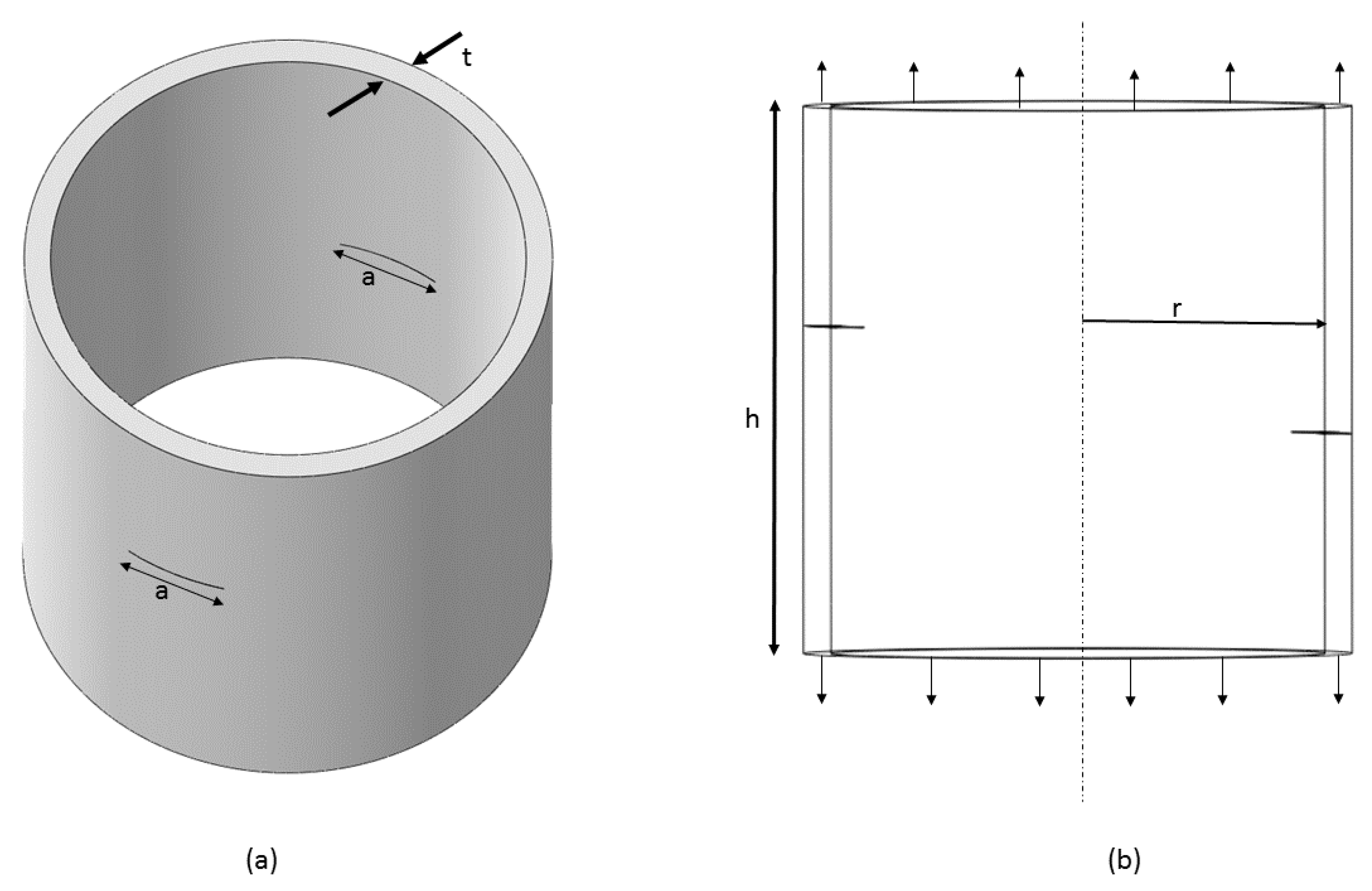
3.6. Crack Propagation in Thick Walled Cylinder

We performed another numerical example to demonstrate the advantages of using the phase-field method to simulate crack propagation. We modeled two parallel cracks at different elevations in a thick walled cylinder under uni-axial tension. The dimensions were: t = 0.1 mm, r = 1 mm, a = 0.2 mm, and h = 1 mm (Figure 14). The material and length scale parameters were: E = 210 kN/mm 2 , ν = 0.2, l c = 0.075 mm, and G c = 2.7 × 10 3 kN/mm. We observed the crack merging phenomenon in this case. The cracks initiated from the respective notches but, when the damage zones were influenced by each other, the two cracks merged (Figure 15). This phenomenon was simulated based on the physics of the system without any ad-hoc criterion set up for the crack propagation path, thereby restating that the phase-field technique can be used to simulate many such cases that would traditionally be a bit more complex using discrete treatment.

4. Discussion

The primary objective of this study was to predict realistic crack paths in three-dimensional solids. The CS-FEM-H8 element is implemented in the commercial platform of ABAQUS. The element was already proven to have a very good accuracy in displacement norm [38]; here, we combined it with the phase-field model for diffuse fracture to simulate crack propagation in 3D linear elastic brittle solids. ABAQUS user elements (UEL) has its inherent limitations in not letting the user access data from surrounding elements, thus we developed a much simpler technique to calculate stress/strain for smoothing domains instead of the traditional weighted average approach. We sacrificed the stress convergence rate due to this new formulation, however still obtained accurate results that predict complex crack topologies such as crack branching and curved crack paths. Several drawbacks of the method were observed during the simulations: the phase-field variable propagation is very much mesh dependent, thus one needs to have a very fine mesh (approximate characteristic element size of ( 1 / 2 ) the length scale parameter, or less [24,25,28]) near the expected crack propagation zone to efficiently resolve the length-scale parameter. This is not an issue for geometries where experimentally obtained crack paths are already known, however, for complex geometries and unknown crack paths, we needed to have a very fine mesh throughout the domain to facilitate independent crack propagation which increases the computational cost. Once the length scale parameter has been successfully resolved, further reduction of the mesh size does not alter the crack path. We also observed that the selection of displacement increment step size affects the resultant crack path. The final fracture pattern is not dependent on the Griffith’s energy release rate parameter, however the ultimate strength of the sample decreases with decreasing G c . Implementation in ABAQUS, as already discussed, has its own drawbacks in not letting the user implement more accurate S-FEM models such as ES-FEM/ α -FEM [18]. This formulation was developed based on the H8 element with eight smoothing cells, which was not generated automatically for complex geometries. Analysts probably need to resort to the use of tetrahedral (T4) elements in cases of complex topologies. This in turn affects the accuracy because the formulations of the T4 elements are the same for both CS-FEM and FEM [1]. However, this opens up an avenue for future research in this domain, where in-house codes can be used to solve the same problem using a much more accurate ES-FEM/FS-FEM and a base mesh of T3/T4 elements, which are very easily generated for complex geometries. Moreover, adaptive meshing schemes designed based on values of the phase-field parameter can be utilized to reduce the computational cost of having very fine mesh. In 2D cases, CS-FEM is slightly more efficient than FEM [39]. However, in this 3D setting, the computational cost is similar (quantitative difference of around 1%) for both FEM and CS-FEM formulations. This is due to the assembly process of the stiffness matrix for each smoothing domain which involves integration over each surface of the cell. However, the better accuracy in the displacement norm and the comparative “soft” property in stiffness matrix with respect to FEM gives CS-FEM an advantage.
Thus, it can be concluded that this method is another efficient and novel computational technique to model crack propagation in 3D structures.

Author Contributions

Formal analysis, S.B.; Investigation, S.B.; Methodology, S.B.; Supervision, G.-R.L.; Validation, S.B.; Writing—original draft, S.B.; and Writing—review and editing, S.B. and G.-R.L.

Funding

This research received no external funding.

Conflicts of Interest

The authors declare no conflict of interest.

References

  1. Liu, G.; Trung, N.T. Smoothed Finite Element Methods; CRC Press: Boca Raton, FL, USA, 2010. [Google Scholar]
  2. Liu, G.R.; Dai, K.Y.; Nguyen, T.T. A smoothed finite element method for mechanics problems. Comput. Mech. 2007, 39, 859–877. [Google Scholar] [CrossRef]
  3. Liu, G.R. Meshfree Methods—Moving Beyond the Finite Element Method; CRC Press: Boca Raton, FL, USA, 2009. [Google Scholar]
  4. Liu, G.R.; Quek, S.S. The Finite Element Method—A Practical Course; CRC Press: Boca Raton, FL, USA, 2003. [Google Scholar]
  5. Liu, G.R.; Nguyen, T.T.; Dai, K.Y.; Lam, K.Y. Theoretical aspects of the smoothed finite element method (SFEM). Int. J. Numer. Methods Eng. 2007, 71, 902–930. [Google Scholar] [CrossRef]
  6. Liu, G.; Nguyen-Thoi, T.; Lam, K. A novel alpha finite element method (αFEM) for exact solution to mechanics problems using triangular and tetrahedral elements. Comput. Methods Appl. Mech. Eng. 2008, 197, 3883–3897. [Google Scholar] [CrossRef]
  7. Liu, G.; Nguyen-Thoi, T.; Nguyen-Xuan, H.; Lam, K. A node-based smoothed finite element method (NS-FEM) for upper bound solutions to solid mechanics problems. Comput. Struct. 2009, 87, 14–26. [Google Scholar] [CrossRef]
  8. Liu, G.; Nguyen-Thoi, T.; Lam, K. An edge-based smoothed finite element method (ES-FEM) for static, free and forced vibration analyses of solids. J. Sound Vib. 2009, 320, 1100–1130. [Google Scholar] [CrossRef]
  9. Zeng, W.; Liu, G.; Jiang, C.; Nguyen-Thoi, T.; Jiang, Y. A generalized beta finite element method with coupled smoothing techniques for solid mechanics. Eng. Anal. Bound. Elem. 2016, 73, 103–119. [Google Scholar] [CrossRef]
  10. Nguyen-Xuan, H.; Rabczuk, T.; Bordas, S.; Debongnie, J. A smoothed finite element method for plate analysis. Comput. Methods Appl. Mech. Eng. 2008, 197, 1184–1203. [Google Scholar] [CrossRef] [Green Version]
  11. Nguyen-Thoi, T.; Liu, G.; Vu-Do, H.; Nguyen-Xuan, H. A face-based smoothed finite element method (FS-FEM) for visco-elastoplastic analyses of 3D solids using tetrahedral mesh. Comput. Methods Appl. Mech. Eng. 2009, 198, 3479–3498. [Google Scholar] [CrossRef]
  12. Nguyen-Thoi, T.; Vu-Do, H.; Rabczuk, T.; Nguyen-Xuan, H. A node-based smoothed finite element method (NS-FEM) for upper bound solution to visco-elastoplastic analyses of solids using triangular and tetrahedral meshes. Comput. Methods Appl. Mech. Eng. 2010, 199, 3005–3027. [Google Scholar] [CrossRef]
  13. Nguyen-Xuan, H.; Liu, G.; Thai-Hoang, C.; Nguyen-Thoi, T. An edge-based smoothed finite element method (ES-FEM) with stabilized discrete shear gap technique for analysis of Reissner–Mindlin plates. Comput. Methods Appl. Mech. Eng. 2010, 199, 471–489. [Google Scholar] [CrossRef]
  14. Nguyen-Thoi, T.; Liu, G.R.; Vu-Do, H.C.; Nguyen-Xuan, H. An edge-based smoothed finite element method for visco-elastoplastic analyses of 2D solids using triangular mesh. Comput. Mech. 2009, 45, 23–44. [Google Scholar] [CrossRef]
  15. Nourbakhshnia, N.; Liu, G.R. A quasi-static crack growth simulation based on the singular ES-FEM. Int. J. Numer. Methods Eng. 2001, 88, 473–492. [Google Scholar] [CrossRef]
  16. Jiun-Shyan, C.; Cheng-Tang, W.; Sangpil, Y.; Yang, Y. A stabilized conforming nodal integration for Galerkin mesh-free methods. Int. J. Numer. Methods Eng. 2000, 50, 435–466. [Google Scholar] [CrossRef]
  17. Nguyen-Xuan, H.; Liu, G.; Bordas, S.; Natarajan, S.; Rabczuk, T. An adaptive singular ES-FEM for mechanics problems with singular field of arbitrary order. Comput. Methods Appl. Mech. Eng. 2013, 253, 252–273. [Google Scholar] [CrossRef]
  18. Bhowmick, S.; Liu, G. On singular ES-FEM for fracture analysis of solids with singular stress fields of arbitrary order. Eng. Anal. Bound. Elem. 2018, 86, 64–81. [Google Scholar] [CrossRef]
  19. Guo, Z.; Liu, Y.; Ma, H.; Huang, S. A fast multipole boundary element method for modeling 2-D multiple crack problems with constant elements. Eng. Anal. Bound. Elem. 2014, 47, 1–9. [Google Scholar] [CrossRef]
  20. Belytschko, T.; Lu, Y.; Gu, L. Crack propagation by element-free Galerkin methods. Eng. Fract. Mech. 1995, 51, 295–315. [Google Scholar] [CrossRef]
  21. Belytschko, T.; Black, T. Elastic crack growth in finite elements with minimal remeshing. Int. J. Numer. Methods Eng. 1999, 45, 601–620. [Google Scholar] [CrossRef]
  22. Zeng, W.; Liu, G.; Kitamura, Y.; Nguyen-Xuan, H. A three-dimensional ES-FEM for fracture mechanics problems in elastic solids. Eng. Fract. Mech. 2013, 114, 127–150. [Google Scholar] [CrossRef]
  23. Liu, G.; Nourbakhshnia, N.; Zhang, Y. A novel singular ES-FEM method for simulating singular stress fields near the crack tips for linear fracture problems. Eng. Fract. Mech. 2011, 78, 863–876. [Google Scholar] [CrossRef]
  24. Bourdin, B.; Francfort, G.; Marigo, J.J. Numerical experiments in revisited brittle fracture. J. Mech. Phys. Solids 2000, 48, 797–826. [Google Scholar] [CrossRef]
  25. Miehe, C.; Hofacker, M.; Welschinger, F. A phase field model for rate-independent crack propagation: Robust algorithmic implementation based on operator splits. Methods Appl. Mech. Eng. 2010, 199, 2765–2778. [Google Scholar] [CrossRef]
  26. Miehe, C.; Welschinger, F.; Hofacker, M. Thermodynamically consistent phase-field models of fracture: Variational principles and multi-field FE implementations. Int. J. Numer. Methods Eng. 2010, 83, 1273–1311. [Google Scholar] [CrossRef]
  27. Molnár, G.; Gravouil, A. 2D and 3D ABAQUS implementation of a robust staggered phase-field solution for modeling brittle fracture. Finite Elem. Anal. Des. 2017, 130, 27–38. [Google Scholar] [CrossRef]
  28. Msekh, M.A.; Sargado, J.M.; Jamshidian, M.; Areias, P.M.; Rabczuk, T. ABAQUS implementation of phase-field model for brittle fracture. Comput. Mater. Sci. 2015, 96, 472–484. [Google Scholar] [CrossRef]
  29. Miehe, C.; Schänzel, L.M. Phase field modeling of fracture in rubbery polymers. Part I: Finite elasticity coupled with brittle failure. J. Mech. Phys. Solids 2014, 65, 93–113. [Google Scholar] [CrossRef]
  30. Miehe, C.; Aldakheel, F.; Raina, A. Phase field modeling of ductile fracture at finite strains: A variational gradient-extended plasticity-damage theory. Int. J. Plast. 2016, 84, 1–32. [Google Scholar] [CrossRef]
  31. Miehe, C.; Schänzel, L.M.; Ulmer, H. Phase field modeling of fracture in multi-physics problems. Part I. Balance of crack surface and failure criteria for brittle crack propagation in thermo-elastic solids. Methods Appl. Mech. Eng. 2015, 294, 449–485. [Google Scholar] [CrossRef]
  32. Miehe, C.; Hofacker, M.; Schänzel, L.M.; Aldakheel, F. Phase field modeling of fracture in multi-physics problems. Part II. Coupled brittle-to-ductile failure criteria and crack propagation in thermo-elastic–plastic solids. Methods Appl. Mech. Eng. 2015, 294, 486–522. [Google Scholar] [CrossRef]
  33. Hofacker, M.; Miehe, C. A phase field model of dynamic fracture: Robust field updates for the analysis of complex crack patterns. Int. J. Numer. Methods Eng. 2012, 93, 276–301. [Google Scholar] [CrossRef]
  34. Borden, M.J.; Verhoosel, C.V.; Scott, M.A.; Hughes, T.J.; Landis, C.M. A phase-field description of dynamic brittle fracture. Methods Appl. Mech. Eng. 2012, 217–220, 77–95. [Google Scholar] [CrossRef]
  35. Rabczuk, T.; Belytschko, T. Cracking particles: a simplified meshfree method for arbitrary evolving cracks. Int. J. Numer. Methods Eng. 2004, 61, 2316–2343. [Google Scholar] [CrossRef]
  36. Areias, P.; Msekh, M.; Rabczuk, T. Damage and fracture algorithm using the screened Poisson equation and local remeshing. Eng. Fract. Mech. 2016, 158, 116–143. [Google Scholar] [CrossRef]
  37. Areias, P.; Rabczuk, T.; de Sá, J.C. A novel two-stage discrete crack method based on the screened Poisson equation and local mesh refinement. Comput. Mech. 2016, 58, 1003–1018. [Google Scholar] [CrossRef]
  38. Nguyen-Xuan, H.; Nguyen, H.V.; Bordas, S.; Rabczuk, T.; Duflot, M. A cell-based smoothed finite element method for three-dimensional solid structures. KSCE J. Civ. Eng. 2012, 16, 1230–1242. [Google Scholar] [CrossRef]
  39. Bhowmick, S.; Liu, G.R. A phase-field modeling for brittle fracture and crack propagation based on the cell-based smoothed finite element method. Eng. Fract. Mech. 2018, 204, 369–387. [Google Scholar] [CrossRef]
  40. Msekh, M.A. Phase Field Modeling for Fracture with Applications to Homogeneous and Heterogeneous Materials. Ph.D. Thesis, Bauhaus-Universität Weimar, Weimar, Germany, 2017. [Google Scholar] [CrossRef]
Figure 1. An arbitrary discontinuous three-dimensional body.
Applsci 08 02488 g001
Figure 2. A 3D H8 element subdivided into eight smoothing cells: (a) subdivision into smoothing cells by joining the midpoints of the edges and the faces; (b) face area of a smoothing cell with its outward normal and length; and (c) entire face of the element containing surfaces of the four smoothing cells.
Applsci 08 02488 g002
Figure 3. A single edge notched tensile specimen: (a) representational 2D geometry; thickness = 2.0 mm; and (b) hexahedral mesh with smaller element size near the expected propagation zone.
Applsci 08 02488 g003
Figure 4. Crack path with increasing time steps.
Applsci 08 02488 g004
Figure 5. Load–displacement curves for varying G c .
Applsci 08 02488 g005
Figure 6. A single edge notched sample under shear loading: (a) panel geometry; (b) crack initiation; (c) crack path after 300 step-times; (d) crack path after 500 step-times; and (e) final crack path.
Applsci 08 02488 g006
Figure 7. A double edge notched tensile sample: (a) 2D Geometric representation of the structure; thickness = 2.0 mm; and (b) biased hexahedral mesh.
Applsci 08 02488 g007
Figure 8. Crack path at different time steps: (a) initial damage after 100 time steps; (b) initial damage after 100 time steps; (c) initial damage after 100 time steps; and (d) final crack path.
Applsci 08 02488 g008
Figure 9. Geometry with notch and openings (in x - y plane): (a) openings are aligned along a straight-line; and (b) openings are aligned haphazardly.
Applsci 08 02488 g009
Figure 10. Crack propagation steps: (a) crack propagation begins (b) crack arrest due to damage from opening; (c) crack propagates through the openings; and (d) crack continues in the previous path.
Applsci 08 02488 g010
Figure 11. Crack propagation steps for higher incremental step size: (a) crack propagation after 100 steps (b) crack propagation through holes; (c) slight bend in path due to damage zone influence of hole below; and (d) propagates along straight path.
Applsci 08 02488 g011
Figure 12. Crack propagation steps for lower incremental step size: (a) crack propagation after 100 steps (b) crack propagation through holes; (c) deflected path due to damage zone influence of hole below; and (d) crack initiates at the stress concentration zone and propagates.
Applsci 08 02488 g012
Figure 13. Crack propagation in a bi-material specimen: (a) representational 2-D geometry; thickness = 5 mm; (b) crack initiation; (c) crack propagation through the soft material; (d) crack reaches the material discontinuity junction; and (e) crack branching.
Applsci 08 02488 g013
Figure 14. Crack propagation in a thick-walled cylinder: (a) isometric view of the cylinder; and (b) relative position of the two Cracks.
Applsci 08 02488 g014
Figure 15. Crack propagation in a thick-walled cylinder: (a) crack initiation; (b) pattern of the two cracks propagating; and (c) final crack merging.
Applsci 08 02488 g015

