Abstract
Vision-based vehicle detection is the most basic and important technology in advanced driver assistance systems. In this paper, we propose a vehicle detection framework using selective multi-stage features in convolutional neural networks (CNNs) to improve vehicle detection performance. A 10-layer CNN model was designed and visualization techniques were used to selectively extract features from the activation feature map, called selective multi-stage features. The proposed features contain characteristic vehicle image information and are more robust than traditional features against noise. We trained the AdaBoost algorithm using these features to implement a vehicle detector. The experimental results verified that the proposed vehicle detection framework exhibited better performance than previous frameworks.
1. Introduction
Vehicle detection has attracted considerable attention in the field of object detection technology, with an increase in the demand for automotive safety and autonomous vehicles and an increase in the number of countries implementing institutional support for driver safety. Reducing the number of traffic accidents directly affects not only human lives, but also many social costs. At the very center of social change are advanced driver assistance systems (ADASs). Vehicle detection is the most basic and important technology underlying ADASs, and vehicle detection research has considerably developed in recent years. On-road vehicle detection has become a significant research topic in the ADAS context with the development of various available sensing technologies (radar, lidar, camera, etc.) and the emergence of multi-core and graphics processing unit (GPU) computing [1]. Vehicle detection is largely divided into technologies that use vision sensors and those that do not. In contrast to other sensors, vision-based vehicle detection can directly recognize vehicles and is a hot research field because of its price advantage.
Vision-based vehicle detection methods can be categorized into appearance- and motion-based methods [2]. Appearance-based methods have been studied extensively for monocular vehicle detection frameworks to recognize the vehicle directly in the image region of interest (ROI). Appearance-based vehicle detection methods extract appearance features from training images to train the classifier using machine learning algorithms and then identify vehicle(s) in the new image ROIs. Many appearance features have been proposed to detect vehicles, including color, symmetry, edges, and histogram of oriented gradients (HOG) features [3]. The following two best practice appearance-based vehicle detection methods have been developed thus far:
- HOG features are extracted from each training image, and the classifier is trained using the support vector machine (SVM) algorithm [4].
- Local binary pattern (LBP) features are extracted from each training image, and the classifier is trained using the adaptive boosting algorithm (AdaBoost) [5].
Motion-based vehicle detection methods generally use optical flow and occupancy grids. Optical flow vehicle detection has been proposed for monocular vehicle detection frameworks [6], and recent dynamic grid processing developments have allowed an efficient use of occupancy grids to monitor highly dynamic scenes; therefore, grids have become a generic tool for obstacle detection [7].
Appearance-based methods generally use monocular vehicle detection, whereas motion-based methods use stereo vehicle detection. The commercial availability of monocular vehicle detection systems means that appearance-based methods have attracted more research and practical application attention than motion-based methods, but they do not provide three-dimensional (3D) depth.
Handcrafted features, such as HOG and LBP, have been widely used by appearance-based vehicle detection methods to discriminate among vehicle images. Handcrafted features are also called middle-level features. Although vehicle detection frameworks that use middle-level features achieve moderate performance, the features are insufficient to fully represent characteristic vehicle image information.
Therefore, in this paper, we propose a vehicle detection framework using a selective multi-stage feature fusion method selectively extracted from convolutional neural networks (CNNs) to improve vehicle detection performance. CNN is a type of deep learning, mainly used to classify images, where vehicle image features are learned in each layer’s feature map. The proposed vehicle detection framework does not use CNN as a classifier, but uses it only to extract specific features in the feature maps of each layer, with the proposed algorithms using visualization techniques. Thus, not only can the characteristic information of the learned features be examined, but the features suitable for vehicle detection can also be selected. We then fuse these selectively extracted features and use AdaBoost to identify vehicle images within the ROI, providing a robust vehicle detection framework. The experiments showed that the proposed vehicle detection framework is more effective than current vehicle detection frameworks that use handcrafted features.
The remainder of this paper is organized as follows: Section 2 describes the related works and the proposed vehicle detection framework. Section 3 defines the experiments and compares the outcomes from the proposed framework and the current best practice frameworks. Finally, Section 4 summarizes and concludes the paper.
2. Vehicle Detection Framework Using Selective Multi-Stage Features
This section details the proposed vehicle detection framework that selectively extracts and fuses features from each CNN layer trained on a vehicle dataset, called selective multi-stage features. In contrast to conventional vehicle detection frameworks, the proposed framework does not use handcrafted features such as HOG or LBP, and the CNN is not used as a classifier, but for feature extraction.
2.1. Related Works
Here, we will describe the basic theory of the CNNs used to selectively extract features in this study.
CNN is an abbreviation for convolutional neural networks and is one of the deep learning models used in image classification and object detection in the field of computer vision. A CNN is a neural network structure for solving the problems of applying the existing multi-layer neural networks to computer vision. Learning 2D images as the input data in the existing multi-layer neural networks takes a long training time, leads to a large network size, and increases the number of free parameters. To solve these problems, the CNN concept was developed on the basis of the human visual cortex. The attribute of a CNN is its ability to utilize local information in a manner similar to that of the receptive field of cells. Therefore, correlation relationships and local features can be extracted using a non-linear filter in the neighboring pixels. By repeating this filter operation with a deep set of layers, the global features can be extracted from the upper layer. In addition, the number of free parameters in a CNN can be reduced as compared to that in the existing multi-neural networks. The CNN was first introduced in 1989 by Yan LeCun [8]. In Reference [8], meaningful results were obtained in handwriting recognition, but there was a limit to the computational power. Then, in Reference [9], the basis of CNN popularization came into being. In this section, we will describe the layers in a CNN and the typical CNN models that should be considered when designing a CNN model.
2.2. Methodology Overview
Figure 1 shows that the proposed vehicle detection framework consists of the training and the detection stages. The training stage includes the following three steps:
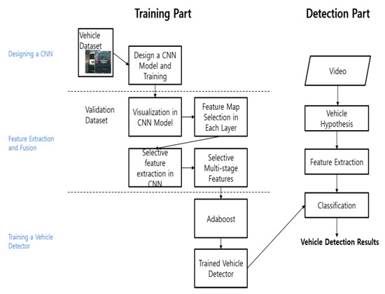
Figure 1.
Proposed vehicle detection framework.
- CNN model design. We designed a CNN model for the proposed vehicle detection framework. The design is important because the features to be extracted depend on the CNN model structure, which should ensure that the characteristic vehicle image information can be learned. We trained the CNN model with a prepared vehicle dataset using the stochastic gradient with momentum and back-propagation algorithms.
- Feature extraction and fusion. We extracted and fused the features containing the characteristic vehicle image information in the trained CNN model using a visualization technique that considered certain aspects of the feature map from each model layer. This step is critical, because the visualization technique implied that we do not need to use all the available feature maps, but can selectively extract features that include only the characteristic vehicle image information.
- Detector training. We trained the detector with the extracted features using the AdaBoost algorithm.
The detection stage included vehicle hypothesis and verification processes. The vehicle hypothesis defined an ROI that was probably a vehicle using a sliding window method. Once the ROI was defined, the trained vehicle detector verified it as either a vehicle or a non-vehicle.
2.3. Designing and Training the CNN Model
The CNN model could be freely designed depending on the application. The purpose of the model in the proposed vehicle detection framework was to selectively extract features reflecting the characteristic vehicle image information from each layer. The feature map aspects learned in the upper and the lower layers differed considerably; therefore, the CNN model had to have sufficient depth to ensure that the lower and the upper layers could be distinguished. The AlexNet [10] characteristics were analyzed by Zeiler and Fergus [11] using Zeiler’s visualization technique and clarified that more than five convolution layers are required to distinguish between the lower and the upper layers. Subsequent CNN research has suggested that very deep CNN models are preferable [12,13]. However, the proposed CNN model was not intended for image classification, but for selectively extracting features representing the vehicle image information from each layer. Therefore, we designed the CNN model with five convolution layers, similar to AlexNet [10] or ZFNet [11].
The factors considered important in the design of the CNN model were the number of filters in the convolution layers and the filter size and stride. More filters meant that more features could be learned from each layer. Furthermore, visualization techniques could be used to systematically identify the patterns of the learned feature maps. Therefore, we designed a CNN model with 60 filters for each convolution layer, each having a size of 5 × 5 pixels and a stride of 1, on the basis of the recent CNN model design trends towards smaller filter sizes and strides [12]. Rectified linear unit (Relu) layers were used to accommodate non-linearity and two max-pooling layers. Table 1 and Figure 2 show the proposed CNN model details.

Table 1.
Proposed convolution neural network (CNN) model parameters.
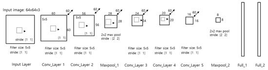
Figure 2.
Proposed CNN Model.
The CNN model was then trained with the prepared vehicle image training dataset, using data augmentation and dropout techniques to prevent overfitting. For data augmentation, we randomly flipped the vehicle images horizontally with 50% probability and took a random crop from the training image with the same size as the input data. The dropout technique omitted some neurons in the input or the hidden layers. For other training options, we set max epochs = 77, initial learning rate = 0.001, and mini batch size = 128. We also used cross-entropy as the cost function and softmax as the activation function.
2.4. Selective Multi-Stage Feature Extraction
In this section, we explain selective feature extraction and fusion using the CNN model designed and trained as described in Section 2.3. The features used for the vehicle detection framework should be robust to geometric transformation and illumination changes and represent the characteristic vehicle image information.
The current features used in the vehicle detection frameworks include the HOG and LBP features. To obtain the HOG features, we divided the input image into cells of a given size, calculated a histogram of the gradient magnitude for each cell, and concatenated the histogram bin values into a 1D vector. As HOG uses gradient information from edges in the input image, it is robust to brightness and illumination changes. Therefore, it is a suitable feature for identifying objects such as people and cars that have clear contour information, but not complicated internal patterns. However, as the HOG feature mainly includes vehicle contour information, it is difficult to say that it contains the characteristic vehicle image information.
The LBP feature is a 1D matrix representing the given-size block histograms of the converted binary index and includes circular texture information, which is robust to illumination changes. However, the original purpose of the LBP feature was to classify image texture; hence, it is difficult to say that the LBP feature contains the characteristic vehicle image information.
The HOG and LBP features are called handcrafted features. Although these are enhanced middle-level features that provide some degree of detection performance over low-level features, such as edges or corners, various new features are emerging that improve vehicle detection performance. Therefore, we propose a feature that can improve vehicle detection performance using selective multi-stage feature extraction and fusion from a CNN. The proposed features effectively reduce dimensionality while including the characteristic vehicle image information and are robust to noise. To selectively extract and fuse features in the CNN model, we must analyze each CNN layer’s feature map. Therefore, we introduced a visualization technique to simplify this task, as shown in Figure 3.
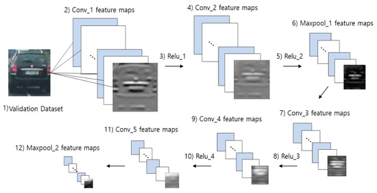
Figure 3.
Proposed visualization technique for the CNN model.
First, we constructed a validation dataset to be used as the input images for the CNN model to visualize the feature map. The validation dataset must not include any images from the training dataset. We investigated the feature maps learned for each CNN layer. When a validation dataset image was input into the trained CNN model, the trained filters in the first convolution layer performed a convolution operation, producing the feature map. The proposed technique visualized these feature maps. The feature maps from the first convolution layer passed through the Relu layer and then to the next convolution layer that performed further convolutions with the previously trained filters, producing the feature map of the second convolution layer. Thus, we obtained the feature maps for all the layers as the image passed through the final convolution layer. Visualizing these feature maps allowed the verification of what vehicle image information was learned as a feature for each layer’s feature map. The visualization technique was essential to selectively extract and fuse features from each layer of the CNN model. Figure 3 shows each numbered layer, and the subsequent sections discuss the feature map visualization in this numerical order to describe the feature map characteristics in each layer.
(1) Verification Dataset
Figure 4 shows a typical example image from the validation dataset that was input into the CNN to visualize the feature maps in the trained CNN model in the subsequent sections.
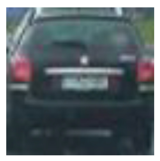
Figure 4.
Sample input image from the validation dataset.
(2) Conv_1 Layer Visualization
There are 60 feature maps in the first convolution. The Conv_1 layer visualization result includes the resultant feature map extracted from the 5 × 5 filter, where the white pixels show significant activation. The first convolution layer extracts the low-level features, such as edge information. Moreover, as it is the initial layer, there is little here that represents the vehicle image characteristics.
(3) Relu_1 Layer Visualization
The first convolution layer feature maps are passed through the Relu function in the Relu_1 layer. As the Relu treats the feature map pixels with value < 0 as 0, the feature map is globally dark. This confirms that only low-level features, i.e., the edge information in the x direction, are learned.
(4) Conv_2 Layer Visualization
There are 60 feature maps in the second convolution layer, and Figure 5a shows the resulting feature map extracted from the 5 × 5 filter, where the white pixels show significant activation. The second convolution layer is also a lower layer, so mainly the low-level features are learned. There are two major differences between the first and the second convolution layer feature maps.
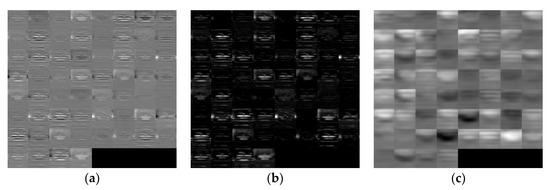
Figure 5.
Example result of CNN’s layer visualizations: (a) Conv_2 Layer Visualization, (b) Maxpool_1 Layer Visualization, (c) Conv_5 Layer Visualization.
- More edge information in the x direction is learned. The feature maps in the second convolution layer represent richer low-level features than those from the first convolution layer. Therefore, when we include low-level features in the fusion process, the second convolution layer feature maps are more appropriate than the first convolution layer ones.
- Some features represent the vehicle head lamp, because the second convolution layer includes the low-level color information features. The head lamp area contains the characteristic vehicle information and can be differentiated from other objects. This particular characteristic information was not found in the other layers. Therefore, the feature map that contains the head lamp information must be included in the fusion process.
(5) Relu_2 Layer Visualization
Relu_2 layer visualization result includes the Relu_2 layer feature maps, produced by passing the second convolution layer through the Relu function. The dark areas are similar to the Relu_1 layer outcome.
(6) Maxpool_1 Layer Visualization
Figure 5b shows the Maxpool_1 layer feature map, which is the result of the max-pooling operation on the feature maps passed through the Relu_2 layer. Max pooling selects only the largest value in the subsampling window. Therefore, Maxpool_1 layer feature maps are stronger and more global than the second convolution or Relu_2 layer feature maps. The feature map visualization is similar to that from the second convolution layer because it is the result of only the max-pooling operation.
(7) Conv_3 Layer Visualization
There are 60 feature maps in the third convolution layer. The Conv_3 layer visualization result includes the resulting feature map extracted from the 5 × 5 filter, where the white pixels show significant activation. Edge information in the x direction is further enhanced, and edge information is concentrated in a specific area of the vehicle image. This is a middle-level feature, intermediate between the low- and the high-level features.
(8) Relu_3 Layer Visualization
The Relu_3 layer visualization result includes the Relu_3 layer feature maps, resulting from passing the third convolution layer feature maps through the Relu function. Dark areas appear, similar to those in the Relu_1 layer maps.
(9) Conv_4 Layer Visualization
There are 60 feature maps in the fourth convolution layer. The Conv_4 layer visualization result includes the resulting feature map extracted from the 5 × 5 filter, where the white pixels show significant activation. The edge information in the x direction is becoming integrated, and this begins to produce a centralized activation around the rear window region of the vehicle image. The global features in the specific narrow region start to be extracted as the high-level features.
(10) Relu_4 Layer Visualization
The Relu_4 layer visualization result includes the Relu_4 layer feature maps, resulting from the fourth convolution layer feature maps passed through the Relu function. Dark areas appear, similar to those in the Relu_1 layer.
(11) Conv_5 Layer Visualization
There are 60 feature maps in the fifth convolution layer. Figure 5c shows the resulting feature map extracted from the 5 × 5 filter, where the white pixels show significant activation. The fifth convolution layer feature maps are focused on the rear window area of the vehicle. Similar to the fourth convolution layer, global features have been learned in a specific narrow area of the vehicle. The difference between the fourth and the fifth convolution layers is that the higher-level features are extracted because of the small feature map dimensions.
(12) Relu_5 Layer Visualization
The Relu_5 layer visualization result includes the Relu_5 layer feature maps, resulting from passing the fifth convolution layer feature maps through the Relu function. Similar to those in the previous Relu feature maps, many dark areas appear.
(13) Maxpool_2 Layer Visualization
The Maxpool_2 layer visualization includes the Maxpool_2 layer feature maps, resulting from max pooling the Relu_5 layer feature maps. Max pooling selects the largest value in the sub-sampling window. The feature map aspects learned are similar to those of the fifth convolution or Relu_5 layer feature maps. Maxpool_2 is the final CNN model layer. Therefore, the Maxpool_2 layer feature map has the smallest dimensionality.
2.5. Selective Multi-Stage Feature Fusion
Visualization steps 1–13 show how the feature map visualizations learned for each layer in the CNN model can be examined. We can identify distinct feature map properties in each layer. However, it is not appropriate to use all these feature maps learned in the CNN model as the vehicle detection feature set. We require an efficient feature set to improve vehicle detection performance while reducing feature dimensionality. Therefore, we propose to fuse selective multi-stage features based on the feature map visualizations, as shown in Section 2.4.
The selective multi-stage feature fusion process was as follows: First, the feature maps were examined using the visualization technique and a few features were selectively extracted from each layer. We then concatenated the selected features into a 1D vector. The criterion for selecting features in each layer was to include the characteristic vehicle image information or to select a feature map with a large activation among the 60 learned feature maps. The characteristic information is an important factor in vehicle detection, because this information is the most effective cue that the detector uses to distinguish whether the target object is a vehicle or non-vehicle. The HOG and LBP features used for conventional vehicle detection frameworks cannot be considered to include the characteristic vehicle image information, because the existing features only use the edge gradient or brightness information. Thus, the proposed fusion of the selective multi-stage feature method differs significantly. Figure 6 shows that information such as the vehicle’s head lamp is the characteristic vehicle image information. Only some of the feature maps among the 60 in Maxpool_1 layer intensively learned the vehicle head lamp information.
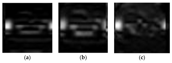
Figure 6.
Characteristic vehicle image information from the Maxpool_1 layer: (a) 24th, (b) 42th, and (c) 45th feature maps.
We selected the feature maps with a large activation because the corresponding feature was the best learned in each layer. Therefore, the proposed selection and fusing of the maximum value feature maps is effective in enhancing vehicle detection performance. Figure 7 shows the maximum value feature maps for each layer. The white pixels show that significant activation for these feature maps is considerably larger than that for the other feature maps in each layer.
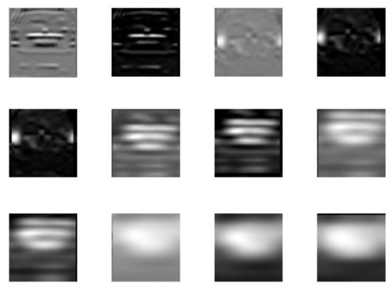
Figure 7.
Maximum value feature maps in each CNN layer.
Thus, considering the feature dimensions to be fused and the characteristic vehicle image information, we extracted features from the Maxpool_1, fourth convolution, and fifth convolution layers, and combined them into a 1D vector to create the feature set for the proposed vehicle detection framework. As several features could be extracted from each layer, we compared performances by fusing features in various combinations, where the best performing feature set was chosen.
2.6. Vehicle Detector Trained by AdaBoost
We trained the detector for the proposed vehicle detection framework using the multi-stage features extracted in Section 2.5 and took advantage of the AdaBoost algorithm. At this time, we selected the decision stumps as a weak classifier of AdaBoost to distinguish whether the input feature is a vehicle or non-vehicle. Freund [14] proposed the adaptive boosting algorithm. It is an aggressive mechanism for selecting a small set of good classification functions, which nevertheless have significant variety [15]. AdaBoost training is iterative. First, we created a weak classifier by inputting the labeled multi-stage features extracted from the CNN. The weight for each input was 1/N, where N is the amount of input data; i.e., all the data had the same weight for the first iteration. The weights of the misclassified data and the weights of the weak classifiers exhibiting good classification performance were iteratively increased. Finally, the weak classifiers were combined to produce the final strong classifier. The training error of the strong classifier approached zero exponentially with the number of iterations [14]. Figure 8 shows the detector training process using the proposed multi-stage features with respect to the AdaBoost algorithm.
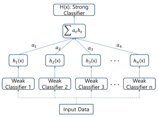
Figure 8.
Vehicle detector training.
3. Experiments and Comparisons
3.1. Environments
The hardware platform used in this study was an Intel dual core i3-6100 processor at 3.70 GHz, with 4 GB memory and Windows 7 operating system. We used the GTI DATA vehicle image database 2012, containing 3425 images of different vehicle rear ends taken from different points of view, and 3900 road sequence images containing no vehicles [16]. All the images were 64 × 64 pixels, and the vehicle and non-vehicle images were considered positive and negative images, respectively. The database contained not only images taken directly behind the vehicle, but also images taken at different angles, in different ranges, and under different lighting conditions. Thus, this database was ideal to create a robust vehicle detection framework, including noise and geometric transformations. We divided the database into the training, test, and validation datasets containing 2950 and 2950, 500 and 975, and 5 and 5 positive and negative images, respectively. Figure 9 shows the typical sample images from the database. Detection error tradeoff (DET) curves were used to evaluate vehicle detection performance. The DET curves were first used to represent the performance of detection tasks that involved a tradeoff of error types [17], contrasting the false positives per window (FPPW) on the horizontal axis and the miss rate on the vertical axis. FPPW is another way of expressing the false alarm rate and represents the average number of false positives per input window; i.e., FPPW is an index indicating how many false positives actually occur. The miss rate is plotted opposite the recall rate; this refers to the ratio of the target object that is not detected among all the target objects in the input data:
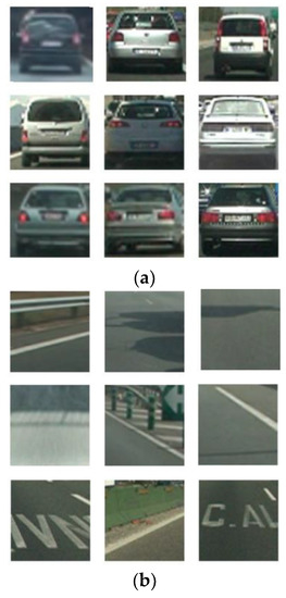
Figure 9.
Typical (a) positive and (b) negative images from the GTI DATA vehicle image database 2012 [16].
We used a logarithmic scale for the DET curves, where better detectors were located closer to the left bottom corner, and FPPW on the horizontal axis was used as a reference point to compare the detector performance.
3.2. Feature Sets
To create a feature set using the proposed selective multi-stage feature method, we compared the feature set dimensions. As discussed above, two criteria were considered for the feature extraction from each CNN layer: The characteristic vehicle image information was included in the trained feature map, and the feature map with the largest activation in each layer was selected. The Maxpool_1, fourth convolution, and fifth convolution layers were selected for the feature extraction, and we input the validation data to the trained CNN model to generate the feature maps for each layer. Three feature maps were selected in the increasing order of the activation value for each layer, as shown in Figure 10 and Table 2.
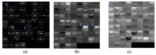
Figure 10.
Top-three activation feature maps selected: (a) Maxpool_1 layer, (b) fourth convolution layer, and (c) fifth convolution layer.
Table 2.
Top-three maximum value features selected for each layer.
3.3. Experiment 1
The first experiment compared the performance depending on the feature combination dimension, using the feature sets shown in Figure 11. Feature set 1 concatenated the first maximum feature map from each layer sequentially (the Maxpoo1, fourth convolution, and fifth convolution layers). Feature set 2 concatenated the first and the second maximum feature maps sequentially, and feature set 3 concatenated all the top three feature maps selected from each layer sequentially. The feature set dimensions were 1440, 2880, and 4320, respectively. Detectors were trained by the AdaBoost algorithm using the three feature sets, and the performance was compared using the DET curves, as shown in Figure 12.
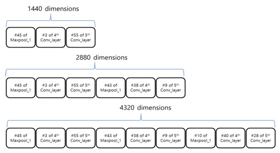
Figure 11.
Feature sets used in the experiment.

Figure 12.
Dimensionality effects.
The performance did not significantly improve when more feature maps with vehicle information were included. We investigated the negative image visualization results to identify the reason. Figure 13 shows the visualizations of the same feature map sequence for each layer for the positive and the negative image samples. Low-level features extracted from the initial layer showed large differences between the positive and the negative images. The 45th feature map in the Maxpool_1 layer, where the headlamp information of the vehicle was extracted, was clearly visible. The same edge information was extracted from the other feature maps in the Maxpool_1 layer, but the edge directions differed. High-level features were extracted from both the positive and the negative image samples for the Conv_4 layer, with the high-level features concentrated in a specific area in each image sample; i.e., the difference between the trained feature maps for the positive and negative image samples was not as significant as that for the initial layer. Finally, the Conv_5 layer, which contained the highest-level features, was extracted. The trained feature maps were similar because the high-level feature was extracted over a narrower specific area than the Conv_4 layer. Thus, the detector performance suffered when we increased dimensionality by concatenating several features with the vehicle image information in the feature set. The larger the number of feature maps from the upper layers (Conv_4 and Conv_5) included in the feature set, the more likely it was that these feature maps would act as noise. Therefore, we chose a 1440-dimensional feature set, including just the maximum feature maps from the Maxpool_1, Conv_4, and Conv_5 layers.
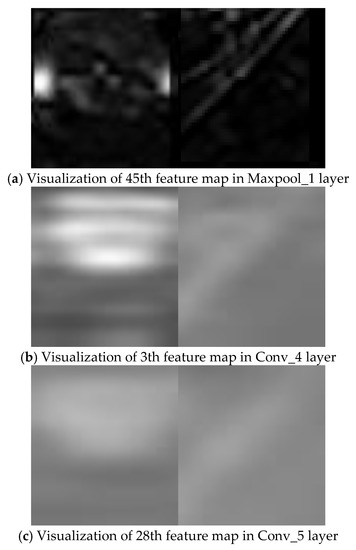
Figure 13.
Positive (left) and negative (right) sample image feature map visualizations.
3.4. Experiment 2
We compared the proposed selected multi-stage feature outcomes to select the most suitable feature combination set for vehicle detection. From the above experiment, the feature set dimensionality was set to 1440. Then, we selected one feature from each of the Maxpool_1, Conv_4, and Conv5_layers (as shown in Figure 10) and constructed the feature sets by concatenating them. Thus, there were 27 possible combinations of the feature set, as shown in Figure 14. We trained the AdaBoost algorithm using the 27 feature set cases and compared their performance using the DET curves, as shown in Figure 15.
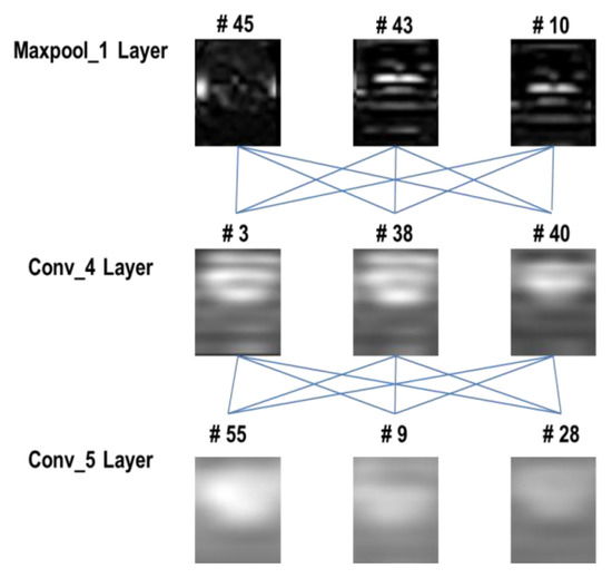
Figure 14.
Feature map combinations.
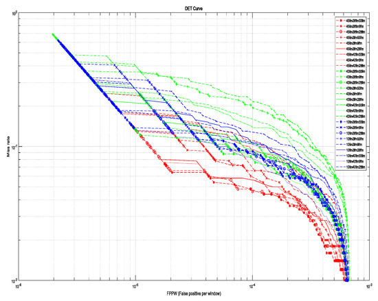
Figure 15.
Feature map combination performances.
The best performance was obtained by combining the Maxpool_1 45th, Conv_4 38th, and Conv_5 55th feature maps. All the outcomes that included the Maxpool_1 45th feature exhibited good performance because this feature map characteristic information included the vehicle head lamps. Thus, feature map inclusion or otherwise of characteristic information regarding the head lamp considerably influenced the performance of the proposed selective multi-stage feature fusion method.
Based on the experimental results, the feature set for the proposed vehicle detection framework was finally selected as the concatenation of the Maxpool_1 45th, Conv_4 38th, and Conv_5 55th feature maps.
3.5. Performance Comparisons
We compared the proposed vehicle detection framework using the selected feature set with the conventional vehicle detection frameworks using HOG, LBP, and HOG + LBP features and a CNN detector. We used AdaBoost to train the detectors for each model and included the second-best performing proposed method detector (as shown in Figure 15).
Figure 16 compares the six models. The proposed vehicle detection framework exhibits the best performance with FPPW. As the selective multi-stage features extracted from the CNN model contained the characteristic vehicle image information, this reduced the false positive rate. The proposed method was more robust to noise than the handcrafted feature methods, even the CNN detector, and provided computational advantages because it had smaller dimensionality than conventional handcrafted methods, requiring 0.07 s to extract the selective multi-stage features, whereas the time taken to extract the LBP and HOG features was 0.0529 s and 0.0926 s, respectively. Thus, the proposed multi-stage feature set extracted from the CNN was the most suitable for vehicle detection.
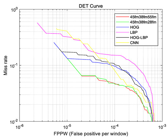
Figure 16.
Proposed and conventional vehicle detection framework performances.
4. Conclusions
In this paper, we proposed a vehicle detection framework consisting of a vehicle hypothesis stage and a vehicle verification stage. The vehicle hypothesis stage uses a sliding window method, and the vehicle verification stage constructs selective multi-stage features extracted from each CNN layer through a visualization technique. We chose an optimal feature set that returned the best vehicle detection performance by comparing feature combinations, and used this feature set as the input for AdaBoost to create the vehicle detector.
To the best of our knowledge, the proposed method is the first system applied to vehicle detection frameworks that creates high-level features that did not exist previously. The experimental results verified that the proposed vehicle detection framework had superior performance to the previous best practice vehicle detection frameworks. In the future, we intend to conduct studies on the generation of more effective selective multi-stage feature sets using different configurations of the training dataset and the test dataset.
Author Contributions
Conceptualization, D.W.K. and M.-T.L.; Funding acquisition, D.W.K. and M.-T.L.; Methodology, W.-J.L. and T.-K.K.; Project administration, T.-K.K.; Supervision, D.W.K. and M.-T.L.; Validation, W.-J.L.; Visualization, T.-K.K. and M.-T.L.; Writing—original draft, W.-J.L.; and Writing—review and editing, D.W.K. and M.-T.L.
Acknowledgments
This research was supported by the Basic Science Research Program through the National Research Foundation of Korea (NRF), funded by the Ministry of Education (Grant Nos. NRF-2016R1D1A1B01016071 and NRF-2017R1D1A1B03031467).
Conflicts of Interest
The authors declare that they have no conflict of interest with respect to this study.
References
- Bila, C.; Sivrikaya, F.; Khan, M.A.; Albayrak, S. Vehicles of the future: A survey of research on safety issues. Int. J. Intell. Transp. Syst. 2017, 18, 1046–1065. [Google Scholar] [CrossRef]
- Sivaraman, S.; Trivedi, M.M. Looking at vehicles on the road: A survey of vision-based vehicle detection, tracking and behavior analysis. Int. J. Intell. Transp. Syst. 2013, 14, 1773–1795. [Google Scholar] [CrossRef]
- Zhu, H.; Yuen, K.V.; Mihaylova, L.; Leung, H. Overview of environment perception for intelligent vehicles. Int. J. Intell. Transp. Syst. 2017, 18, 2584–2601. [Google Scholar] [CrossRef]
- Teoh, S.S.; Braunl, S.T. Symmery-based monocular vehicle detection system. Mach. Vis. Appl. 2012, 23, 831–842. [Google Scholar] [CrossRef]
- Neumann, D.; Langner, T.; Ulbrich, F.; Spitta, D.; Goehring, D. Online vehicle detection using Haar-like, LBP and HOG feature based image classifiers with stereo vision preselection. In Proceedings of the Intelligent Vehicles Symposium (IV), Anchorage, AK, USA, 11–14 June 2017; pp. 773–778. [Google Scholar]
- Martinez, E.; Diaz, M.; Melenchon, J.; Montero, J.; Iriondo, I.; Socoro, J. Driving assistance system based on the detection of head-on collisions. In Proceedings of the IEEE Intelligent Vehicles Symposium, Eindhoven, The Netherlands, 4–6 June 2008; pp. 913–918. [Google Scholar]
- Perrollaz, M.; Yoder, J.D.; Negre, A.; Spalanzani, A.; Laugier, C. A visibility-based approach for occupancy grid computation in disparity space. Int. J. Intell. Transp. Syst. 2012, 13, 1383–1393. [Google Scholar] [CrossRef]
- Lecun, Y.; Boser, B.; Denker, J.S.; Henderson, D.; Howard, R.E.; Hubbard, W.; Jackel, L.D. Backpropagation applied to handwritten zip code recognition. Neural Comput. 1989, 1, 541–551. [Google Scholar] [CrossRef]
- Simard, Y.; Steinkraus, D.; Platt, J.C. Best practices for convolutional neural networks applied to visual document analysis. In Proceedings of the 7th International Conference on Document Analysis and Recognition, Edinburgh, UK, 3–6 August 2003. [Google Scholar]
- Krizhevsky, A.; Sutskever, I.; Hinton, G.E. ImageNet classification with deep convolutional neural networks. In Proceedings of the 25th International Conference on Neural Information Processing Systems, Lake Tahoe, NV, USA, 3–6 December 2012; pp. 1097–1105. [Google Scholar]
- Zeiler, M.D.; Fergus, R. Visualizing and Understanding Convolutional Networks; Lecture Notes in Computer Science; Springer: Cham, Germany, 2014; Volume 8689. [Google Scholar]
- Simonyan, K.; Zisserman, A. Very deep convolutional networks for large-scale image recognition. In Proceedings of the 2nd International Conference on Learning Representations, Banff, AB, Canada, 14–16 April 2014; pp. 1–14. [Google Scholar]
- Szegedy, C.; Liu, W.; Jia, Y.; Sermanet, P.; Reed, S.; Anguelov, D.; Erhan, D.; Vanhoucke, V.; Rabinovich, A. Going deeper with convolutions. In Proceedings of the IEEE Computer Society Conference on Computer Vision and Pattern Recognition, Boston, MA, USA, 7–12 June 2015. [Google Scholar]
- Freund, Y.; Schapire, R.E. A detection-theoretic generalization of on-line learning and an application to boosting. Int. J. Comput. Syst. Sci. 1997, 55, 119–139. [Google Scholar] [CrossRef]
- Viola, P.; Jones, M.J. Robust real-time face detection. Int. J. Comput. Vis. 2004, 57, 137–154. [Google Scholar] [CrossRef]
- The GTI-UPM Vehicle Image Database. Available online: https://www.gti.ssr.upm.es/data/Vehicle_database.html (accessed on 1 December 2017).
- Martin, A.; Doddington, A.G.; Kamm, T.; Ordowski, M.; Przybocki, M. The DET curve in assessment of detection task performance. In Proceedings of the 5th European Conference on Speech Communication and Technology (EUROSPEECH ’97), Rhodes, Greece, 22–25 September 1997; pp. 1895–1898. [Google Scholar]
© 2018 by the authors. Licensee MDPI, Basel, Switzerland. This article is an open access article distributed under the terms and conditions of the Creative Commons Attribution (CC BY) license (http://creativecommons.org/licenses/by/4.0/).