Article

Comparison of Relaxation Modulus Converted from Frequency- and Time-Dependent Viscoelastic Functions through Numerical Methods

1
School of Transportation, Southeast University, Nanjing 211189, China
2
College of Engineering, Tibet University, Tibet 850000, China
*
Authors to whom correspondence should be addressed.
Appl. Sci. 2018, 8(12), 2447; https://doi.org/10.3390/app8122447
Submission received: 2 October 2018 / Revised: 15 November 2018 / Accepted: 19 November 2018 / Published: 1 December 2018
(This article belongs to the Special Issue Asphalt Materials)

Abstract

:
Due to the difficulty of obtaining relaxation modulus directly from experiments, many interconversion methods from other viscoelastic functions to relaxation modulus were developed in previous years. The objectives of this paper were to analyze the difference of relaxation modulus converted from dynamic modulus and creep compliance and explore its potential causes. The selected methods were the numerical interconversions based on Prony series representation. For the dynamic to relaxation conversion, the time spectrum was determined by the collocation method. Meanwhile, for the creep to relaxation conversion, both the collocation method and least squares method were adopted to perform the Laplace transform. The results show that these two methods do not present a significant difference in estimating relaxation modulus. Their difference mostly exists in the transient reduced time region. Calculating the average of two methods is suggested to avoid great deviation of single experiment. To predict viscoelastic responses from creep compliance, the collocation method yields comparable results to the least squares method. Thus, simply-calculated collocation method may be preferable in practice. Further, the master curve pattern is sensitive to the Prony series coefficients. The difference in transient reduced time region may be attributed to the indeterminate Prony series coefficients.

1. Introduction

Asphalt mixtures exhibit viscoelastic behaviors over a wide range of time and temperatures. The responses characterizing the time- and frequency- dependent viscoelastic properties of asphalt mixtures include dynamic modulus, creep compliance and relaxation modulus. These parameters can not only be used to describe the linear viscoelastic properties, but also can indicate the nonlinear viscoelastic properties and failure properties of materials. In fact, these three properties can be interconverted between time- and frequency- domains because linear viscoelastic material properties shared an equivalent mathematical theory, including differential and integral equations [1,2,3].
Dynamic modulus is mathematically defined as the maximum dynamic stress divided by the peak recoverable axial strain, and is a key input for the prediction of field rut depth or fatigue crack amount in the current AASHTOWare pavement ME design program. Creep compliance describes the phenomenon that strain decreases with time under constant stress. In contrast, relaxation describes the phenomenon that stress decreases with time under constant strain. Relaxation modulus is required to calculate thermal stress within asphalt pavement structure in finite element analysis and in the pavement design procedure [4]. However, the direct test of relaxation modulus is typically time- and cost-consuming, as the constant-strain is difficult to control in experiments, whereas it is relatively more convenient to measure the dynamic modulus and creep compliance in laboratory with high testing accuracy. Thus, relaxation modulus in most cases is obtained from dynamic modulus or creep compliance by conversion methods.
The master curve of dynamic modulus or creep compliance needs to be determined before converting to relaxation modulus. Different mathematical functions can be used to obtain master curve, such as pure power law, generalized power law, modified power law, and Prony series [5]. The pure power law, generalized power law, and modified power law have their own benefits, such as being easy to implement, or can be better used to represent the transition zone of a master curve. However, they were not selected since they are not suitable for characterizing short-term or long-term properties [6,7]. Prony series was selected in this paper since it has been widely proved to best represent the fitting equations of master curve [8]. Prony series is a mathematical method to fit a set of equidistant data based on a series of damped complex exponentials. It is widely used in linear viscoelastic material functions, since it can significantly improve the computational efficiency attributed to its physical basis in the theory of mechanical models dealing with linear springs and dashpots [9].
The interconversion between dynamic modulus and relaxation modulus was firstly proposed by Schapery [3]. Later, Cost and Becker [10] proposed the least squares method to directly fit the Prony series to experimental data. However, during these conversions, negative coefficients cannot be avoided, which may generate oscillations in the master curve. To solve the issue, Park and Kim [2] introduced constraints to ensure that all the Prony series coefficients are positive so that a smooth master curve could be plotted. Before fitting the Prony series, modification technologies such as pre-smoothing raw data was proved to portray a smoother curve over a wide range of time [4,11]. Recently, researchers have been developing methods to generate relaxation modulus with no need to use the collocation method or the least squares method, such as semi-analytical algorithm and Levenberg-Marquardt method [12,13,14].
The relaxation modulus can be obtained from the creep compliance through numerical or analytical approaches, which have been developed by several researchers [15,16,17,18]. In regards to exact analytical interconversion, the integral solution usually can be achieved in an infinite range. However, the experimental data can only be collected in a limited range. Thus, it is highly possible to get complicated expressions in the process of solving integrals [5]. Therefore, researchers proposed different approximate analytical methods to simplify the integral computation procedure, such as quasi-elastic relationship, power-law, Prony series, and interrelationship [15,16,17,19,20]. It is generally accepted that numerical method based on Prony series is easier to implement in contrast to the exact analytical method, and it is also more accurate than the approximate analytical method [21,22].
With various fitting approaches available, it is of great interest to compare the accuracy and efficiency of those approaches for the same group of testing results to help identify more appropriate method. In previous studies, despite the overall performance of converted relaxation modulus being acceptable, uncertain difference still often occurred. The performance of relaxation modulus converted from both dynamic modulus and creep compliance based on the same specimens was rarely compared. Thus, the objective of this paper was to adopt the numerical method based on Prony series to obtain relaxation modulus from dynamic modulus and creep compliance. The Prony series representations of these viscoelastic functions were introduced first. Then, rationale of the interconversion methods was elaborated. Finally, numerical examples were presented to compare the difference of two methods.

2. Methodology

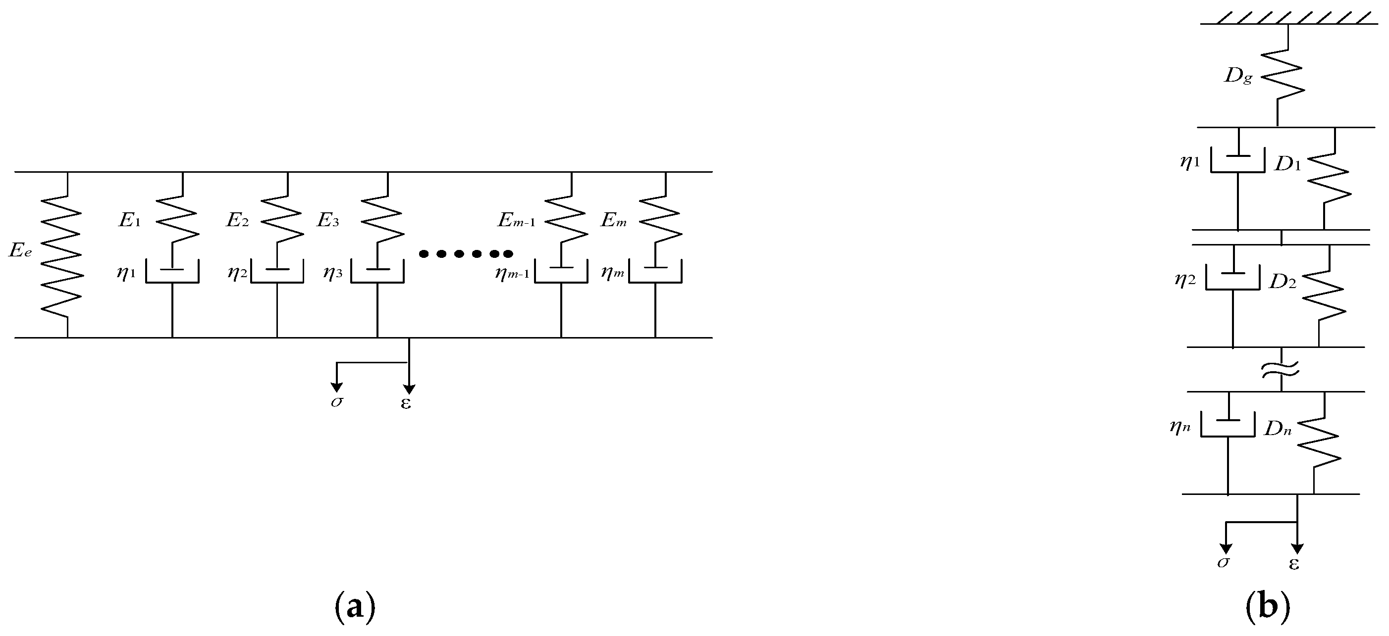
2.1. Viscoelastic Response Representations

The viscoelastic responses of asphalt mixtures can be expressed by combination of spring and dashpot [23]. The generalized Maxwell model consisting of a spring and m Maxwell elements installed in parallel in Figure 1a can be used to depict the total stress of asphalt mixtures. Differentiating its strain based on elastic theory [15], the Prony series representation of complex modulus (E*) can be determined as follows:
E * = E e + i = 1 m i ω ρ i E i i ω ρ i + 1
where E e is the equilibrium modulus, E e = lim t E ( t ) , MPa; i is the complex number, i = 1 ; ω is the angular frequency, rad/s; E i are the relaxation strengths, MPa; ρ i are the relaxation times, ρ i = η i / E i , s; η i is the viscosity of dashpot in a Maxwell element.
Creep compliance is the ratio of strain and stress under certain temperature and stress. It can be depicted by the generalized Kelvin model consisting of a spring and a dashpot and n Kelvin elements connected in series in Figure 1b. The Prony series representation of creep compliance (D(t)) can be expressed by:
D ( t ) = D g + j = 1 n D j [ 1 e ( t / τ j ) ]
where D g is the glassy compliance, 1/MPa; D j are the retardation strengths, 1/MPa; τ j are the retardation times, s.
In contrast, relaxation modulus is the ratio of stress and strain. It is also derived from the generalized Maxwell model and its Prony series representation is given by:
E ( t ) = E e + i = 1 m E i e ( t / ρ i )

2.2. Interconversion Relationship between Time-Domain and Frequency-Domain Functions

Under uniaxial, nonaging and isothermal conditions, the linear viscoelastic behavior of asphalt mixtures can be depicted by Boltzmann superposition integral [1]:
σ ( t ) = 0 t E ( t τ ) d ε ( t ) d τ d τ
ε ( t ) = 0 t D ( t τ ) d σ d τ d τ
where σ, ε denote stress and strain, respectively; τ Means the integral variable of time. Substituting Equation (5) to Equation (4) can derive the constitutive model of relaxation modulus and creep compliance in time region [24]:
0 t E ( t τ ) d D ( τ ) d τ d τ = 1
Then, the relationship of relaxation modulus and creep compliance in Laplace transform domain [15] can be obtained:
E ¯ ( s ) D ¯ ( s ) = 1 / s 2 ,   E ˜ ( s ) D ˜ ( s ) = 1
where f ¯ ( s ) is the Laplace transformation of f ( t ) , f ¯ ( s ) = 0 f ( t ) e s t d t ; s is the Laplace operator; E ˜ ( s ) is the Laplace transform of relaxation modulus, E ˜ ( s ) = s E ¯ ( s ) ; D ˜ ( s ) is the Laplace transform of creep compliance, D ˜ ( s ) = s D ¯ ( s ) .
Since the complex function of viscoelastic materials is excited by sinusoidal loading under ω angular frequency, the relationship between it and Laplace transformed function can be found as [25]:
E * ( ω ) = E ˜ ( s ) | s i ω ,   D * ( ω ) = D ˜ ( s ) | s i ω
where E* is the complex modulus; D* is the complex compliance.
Thus, relationship between E * and D * can be given by:
E * ( ω ) D * ( ω ) = 1
As mentioned above, the time-domain and frequency-domain interrelationship can be derived based on linear viscoelastic theory. Thus, in the following section, relaxation modulus converted by dynamic modulus and creep compliance will be conducted according to this principle.

2.2.1. Interconversion from Dynamic Modulus to Relaxation Modulus

The dynamic modulus and relaxation modulus sheared same Prony series coefficients, thus, the Prony series coefficients of relaxation modulus can be directly acquired by fitting master curve of dynamic modulus. Direct fitting of dynamic modulus is extremely difficult since the equation is the sum of storage modulus and loss modulus which cannot be directly expressed. Fitting dynamic modulus includes fitting the two components of dynamic modulus: Storage modulus and loss modulus. The Prony series by fitting either storage modulus or loss modulus can be used as the Prony series for dynamic modulus since dynamic modulus, storage modulus and loss modulus shared the same Prony series as shown in Equations (1) and (11). However, as shown in Equation (11), the fitting process of storage modulus can give the result of Ee which is a required parameter to calculate relaxation modulus in Equation (3), whereas the fitting process of loss modulus cannot. Thus, the fitting of storage modulus was applied to obtain the Prony series of dynamic modulus. Here, the storage modulus in viscoelastic materials measures the stored energy, representing the elastic portion, and the loss modulus measures the energy dissipated as heat, representing the viscous portion. Equation (10) shows the relationship between complex modulus, storage modulus, and loss modulus.
E * = E + i E
In Equation (10), E is the storage modulus; E is the loss modulus.
According to the representation of complex modulus in Equation (1), the storage modulus and loss modulus can be found as:
E ( ω ) = E e + i = 1 m ω 2 ρ i 2 E i ω 2 ρ i 2 + 1 ,   E ( ω ) = i = 1 m ω ρ i E i ω 2 ρ i 2 + 1
Therefore, the procedure of interconversion from dynamic modulus to relaxation modulus is available:
(1)
Pre-smooth and fit the experimental data of dynamic modulus and phase angle;
(2)
Calculate the storage modulus E e x p r i m e n t based on experimental data;
(3)
Make the storage modulus E p r e d i c t determined by Equation (11) equal to the E e x p r i m e n t so as to obtain Prony series coefficients E e and E i ;
(4)
Substitute E e and E i into the relaxation modulus representation to plot its master curve over a wide time region.

2.2.2. Interconversion from Creep Compliance to Relaxation Modulus

As noted above, Equation (6) reveals the relationship between creep compliance and relaxation modulus in Laplace transform domain. Accordingly, relaxation modulus can be converted by creep compliance based on this formula in the following.
Substituting the Prony series representations of relaxation modulus and creep compliance into Equation (6), the integral can be expressed by:
0 t E e + i m E i e [ ( t τ ) / ρ i ] ( D g δ ( t ) + j n D j τ j e ( t / τ ) ) d τ = 1
where δ (   ) is the Dirac delta function.
According to the literature [15], further simplifying the integral can derive the following equations:
{ i = 1 m [ j = 1 n ρ i D j ρ i τ j ( e ( t / ρ i ) e ( t / τ j ) ) + D g e ( t / ρ i ) ] E i = 1 ( D g + j = 1 n D j ( 1 e ( t k / τ j ) ) ) E e , ρ i τ j i = 1 m [ j = 1 n t D j τ j e ( t / ρ i ) + D g e ( t / ρ i ) ] D j = 1 ( D g + j = 1 n D j ( 1 e ( t k / τ j ) ) ) E e       , ρ i = τ j
where,
E e lim t E ( t ) = lim s 0 E ˜ ( s ) = 1 lim s 0 D ˜ ( s ) = 1 lim t D ( t ) = 1 D g + j = 1 n D j
Adjusting them into linear system of equations, Equation (15) can be given as:
[ A ] [ E ] = [ B ] A k i = { D g e ( t k / ρ i ) + j = 1 n ρ i D j ρ i τ j ( e ( t k / ρ i ) e ( t k / τ j ) ) , ρ i τ j D g e ( t k / ρ i ) + j = 1 n t k D j τ j ( e ( t k / ρ i ) )      , ρ i = τ j B k j = 1 ( D g + j = 1 n D j ( 1 e ( t k / τ j ) ) ) / ( D g + j = 1 n D j )
In Equation (15), matrix [E] denotes the collection of E i for relaxation modulus, which can be derived from matrix operation between matrix [A] and matrix [B]. Time spectrum t k ( k = 1 , 2 , ... , p ) denotes the upper limit of integral in Equation (12) and can be identified through the collocation method or the least squares method. In the collocation method, the number of t k must be equal to E i , whereas the number of t k could be more than E i in the least squares method. In that case, the linear system may be overdetermined equations, and the exact solution cannot be reached. Thus, the optimal solution for it may be effective by calculating in MATLAB to minimize A E B 2 .
Consequently, the procedure of the converted relaxation modulus from creep compliance can be given as:
(1)
Pre-smooth the experimental data of creep compliance and fit its Prony series coefficients D g and D j ;
(2)
Calculate the Prony series of relaxation modulus based on [E] = [A]−1[B] by converting D g and D j to E e and E i ;
(3)
Substitute E e and E i into the relaxation modulus representation to plot the master curve of it over a wide time region.

3. Numerical Examples

3.1. Experiments Design

In the experiment, selected specimen is hot mix asphalt AC-13. The performance grade of asphalt binder is PG70-22. The aggregate gradation of tested HMA can be seen in Table 1.
The specimen was compacted by Superpave Gyratory Compactor (SGC). The cylindrical AC sample was 150 mm in diameter and 170 mm in height. Then, these samples were core-drilled and sawed to finished specimens with 100 mm in diameter and 150 mm in height. Three duplicated specimens were prepared for repeated experiments and the air voids were controlled between 4% ± 0.5%. Having prepared the specimens, they were heated up to experimental temperature and preserved for one hour, then the dynamic modulus and creep compliance were measured.
The dynamic modulus and creep compliance were obtained by uniaxial compression tests which were conducted on Material Testing System (MTS). The vertical deformation was measured by four linear variable differential transducers (LVDT) at 90° radial intervals with a 90 mm gauge length. In the dynamic modulus test, the maximum axial and horizontal strain was controlled in 100 με. The test was conducted under four different temperatures of 4.4 °C, 21.1 °C, 37.8 °C and 54.4 °C according to AASHTO PP61 for the preparation of plotting master curve of dynamic modulus. Also, nine different frequencies of 0.1Hz, 0.2 Hz, 0.5 Hz, 1.0 Hz, 2.0 Hz, 5.0 Hz, 10.0 Hz, 20.0 Hz and 25.0 Hz were under sinusoidal loading at each temperature. The loading time is 100 s and time intervals are 5 min at each temperature. The experimental data of dynamic modulus and phase angle was determined by the average of four LVDTs and the results were the average of three repeated experiments.
After dynamic modulus test, the specimens were required to stand for one hour waiting for deformation recovery. Then, the creep compliance test can be conducted. The specimens were tested under −20 °C, −10 °C, 0 °C, 10 °C, 20 °C and 30 °C. And 100 s at each temperature. The horizontal strain was controlled in 100   μ ε . The results were also the average of three repeated experiments.

3.2. Experimental Data Processing

As designed in the experiments, the micro-strain of specimen under different frequency is around 100 με. Moreover, the measured dynamic modulus and phase angle is constant under changeable loading. Thus, the experiments can be regarded as non-destructive ones that can maintain the specimen within linear viscoelastic range [26].
According to the time-temperature superposition principle, dynamic modulus and phase angle under different temperatures and frequencies can be translated to an integrated curve, called master curve [27]. Therefore, to obtain a dynamic modulus master curve, the curves under different temperatures are required to be horizontally shifted to one curve at a given temperature [28]. In this case, the long-term mechanical behavior of the asphalt material can be predicted without having to perform experiments for a long duration of testing time. In addition, the mechanical behavior of the material is at very short loading times (or very high frequencies) which are difficult to obtain from the experiments can be determined using the master curve [29].
Sigmoid functions as Equation (16) can be employed to pre-smooth the discrete experimental data of dynamic modulus. Similarly, Equation (17) can be used to pre-smooth the discrete experimental data of phase angle [30]. The function of calculating the reduced frequency can be obtained through Equation (18). The reduced frequency is defined as the computed frequency at the reference temperature, equivalent to the actual loading frequency at the test temperature. All of these fitted parameters can be determined by fitting the functions to experimental data and the summary of the fitted results are shown in Table 2.
log | E * | = δ + α ( 1 + e β + γ log ( f r ) )
δ ( f r ) = ξ 1 + ξ 2 log ( f r ) ξ 3 π 2 α γ e β + γ log ( f r ) ( 1 + e β + γ log ( f r ) ) 2
log ( f r ) = log ( f ) + log ( α T )
where, f r is the reduced frequency; f is the loading frequency; δ is the minimum modulus; α is the parameter of vertical span of dynamic modulus; β, γ are the shape parameters of the material; ξ 1 , ξ 2 , ξ 3 are all fitting parameters of experimental data; α T is the time-temperature shifting factor.
The determination of α T is based on Williams-Landel-Ferry (WLF) model [28] in Equation (19).
log ( α T ) = C 1 ( T T 0 ) C 2 + ( T T 0 )
where C1 and C2 are the WLF coefficients; T is the testing temperature; T0 is the reference temperature, which indicates that temperature at which the master curve is constructed.
Thus, after the processing of experimental data, dynamic modulus and phase angle master curves at 21.1 °C Reference Temperature of asphalt mixtures can be obtained as presented in Figure 2.
Similar to the process of fitting master curves of dynamic modulus and phase angle, the creep compliance master curve can be found as in Figure 3. Considering the requirement of comparison between dynamic modulus and creep compliance interconversions, the reference temperature is required to be the same.

3.3. Interconversions

3.3.1. Dynamic Modulus to Relaxation Modulus

Regarding to the procedures of interconversion from dynamic modulus to relaxation modulus, storage modulus is needed to be calculated based on Equation (12). In the equation, relaxation times ρ i is expected to be identified first. According to reference [3], the distribution of ρ i could be estimated through the collocation method. Moreover, in general terms, the integrated curves could be smoother with smaller relaxation time interval. The logarithmic time interval lower than 0.5 is recommended [2]. However, the curve oscillation has already reached an acceptable range when the logarithmic time interval is less than 1 [15]. Therefore, the logarithmic time interval 1 will be employed in the following computation. Another important issue is the number of Maxwell elements, more elements yields to higher accuracy in general, but leading to more complexity at the same time [31]. Usually, 10 elements are enough for the transformation [32]. Therefore, to span enough time range of the data, 11 elements will be taken, meaning that ρ i = 2 × 10 i 7 s ,   i = 1 , 2 , ... , 11 . Consequently, the Prony series coefficients converted by dynamic modulus are listed in Table 2.

3.3.2. Creep Compliance to Relaxation Modulus

Before converting creep compliance to relaxation modulus, the retardation times of creep compliance need to be determined by the collocation method. Compared with the relaxation times ρ i of dynamic modulus, the same number of elements 11 is selected to describe retardation times τ j of creep compliance.
Time constants t k are also required which can be determined by the collocation method or the least squares method [15]. The number of time constants t k was also selected as 11 to keep consistency with the number of retardation times. However, in the least square method, t k = 2 × 10 ( k 1 ) / 2 6 s , k = 1 , 2 , ... , 21 . Therefore, in the collocation method, matrix A is 11 × 11 and matrix B is 11 × 1, whereas in the least square method, matrix A is 20 × 11 and matrix B is 20 × 1, both matrix calculations were completed in software MATLAB. As can be seen, the matrix utilized in the least square method is more complicated and required more computational time in contrast to the collocation method.
Regarding the interconversion from creep compliance to relaxation modulus, τ j was firstly determined and it was assumed that τ j and ρ i are equivalent as suggested [33]. In this paper, τ j was selected between 2 × 10⁶ to 2 × 10⁻⁴ to cover the entire range of relaxation modulus. Theoretically, the relaxation times ρ i are the negative reciprocal of s when E ˜ ( s ) approaches to infinite [15]. The ρ i can also be determined by root-finding method based on | E ˜ ( s ) | versus 1 / s figure, whereas the calculated ρ i was almost identical by using the two methods: assuming τ j is equivalent to ρ i , and root-finding method [4,34]. The Prony series coefficients of creep compliance and relaxation modulus are finally calculated in software MATLAB and results are listed in Table 3.

3.4. Discussion of Results

Based on the above procedures, the results of the two numerical interconversion methods can be analyzed. Before comparing the results of relaxation modulus converted from dynamic modulus and creep compliance, it needs to determine which method is better to represent the creep to relaxation conversion results. The collocation method was adopted in the transferring dynamic modulus to relaxation modulus, whereas both collocation method and least squares method were adopted in the transferring creep compliance to relaxation conversion.
Figure 4 compares the relaxation modulus obtained by the collocation method and squares method. The relaxation modulus from collocation method was compared with relaxation modulus from least squares method based on statistical t-test at a significance level of 0.05. Results indicate that there was no statistical difference between relaxation modulus based on the two methods. In other words, the relaxation modulus converted from creep compliance through the collocation method and least squares method is almost the same.
Assuming the collocation method is more reliable, the relaxation modulus converted through it can be selected to represent the creep to relaxation conversion results. Combined with the dynamic to relaxation conversion results, these two curves can be compared in Figure 5 in semi-log scale.
Figure 5a is plotted by using semi-log scale in which a clear pattern of relaxation can be observed: the relaxation modulus dramatically reduced within a short period and then tends to plateau. Figure 5b is plotted by using log-log scale in which the relationship between relaxation modulus and reduced time at a wide range is available. The relaxation modulus difference based on dynamic modulus and creep compliance was also calculated. As seen, such a difference was relatively small at the short- or long-term region, whereas the difference greatly increased in the middle part of reduced time. The difference curve also presents to be fluctuated. Meanwhile, it is noted that the relaxation modulus appears a three-phase feature in the log-log scale and presents approximately linearity in the transition region. Again, statistical t-test at a significance level of 0.05 was conducted and results indicate that there was no statistical difference between relaxation modulus based on the two methods.
Since the methods adopted are numerical methods, the accuracy is directly related to the number of mechanical model elements. In the context of 11 elements, there are still obvious difference despite the results are similar overall. It is also proved that the difference mostly lies in the lower reduced time range. Due to the same specimens were tested for these two methods, the specimen to specimen variation may not be the determinant factor. A potential reason may be the error of fitting Prony series coefficients in lower reduced time region. The master curve pattern is sensitive to the Prony series coefficients. However, the experimental data is discrete and hard to get continuous and accurate processed data. Pre-smoothing the raw data can improve the performance of obtaining more consistent Prony series coefficients but also may generate some deviation in the Prony series coefficients fitting. Therefore, the difference curve may present to be fluctuated and does not have an obvious rule.

3.5. Validation of the Methodology

To validate the relaxation modulus conversion methods mentioned above, data points from another research project are adopted in this paper for validation purposes. The test specimen was gyratory compacted using loose mixture from field asphalt plant. Three types of additives were adopted to modify neat binders, namely Evotherm, rubber, and polymer. Both dynamic modulus and creep compliance of specimen was tested using the same test apparatus, test temperatures and frequencies as specified in Section 3.1. Relaxation modulus was converted by using both dynamic modulus and creep compliance. Table 4 presents the Prony series coefficients of relaxation modulus of the three mixture types.
Figure 6a–c show the master curve and percentage difference caused by dynamic modulus and creep compliance, respectively. As can be seen, the two master curves of relaxation modulus obtained by dynamic modulus and creep compliance are close to each by visual observation. The difference ranges are 1% to 28% for the specimens using Evotherm modified binders, 2% to 35% for the specimens using rubber modified binders, and 7% to 32% for the specimens using polymer modified binders, respectively. The validation results confirm that the methods used in this paper are robust.

4. Conclusions

This study compared the relaxation modulus converted form dynamic modulus and creep compliance based on the same HMA specimens. To save testing costs and obtain more accurate viscoelastic parameters of asphalt mixture at a wider range, some conclusions can be illustrated:
  • For the transition of creep compliance to relaxation modulus, using the collocation method and least squares method is quite related. However, the collocation method is not as complex as the least squares method. Thus, the collocation method may be preferable in practice.
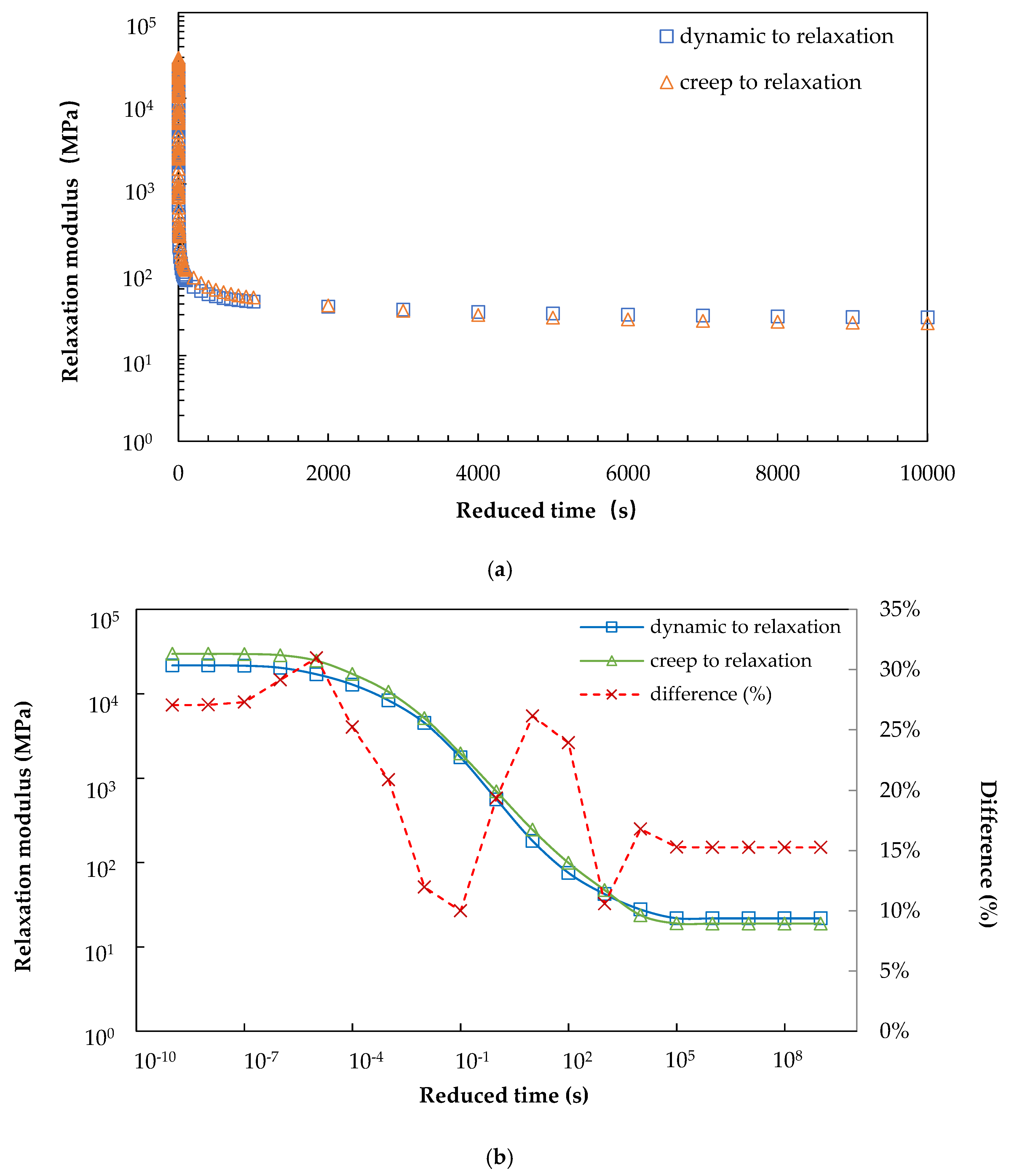
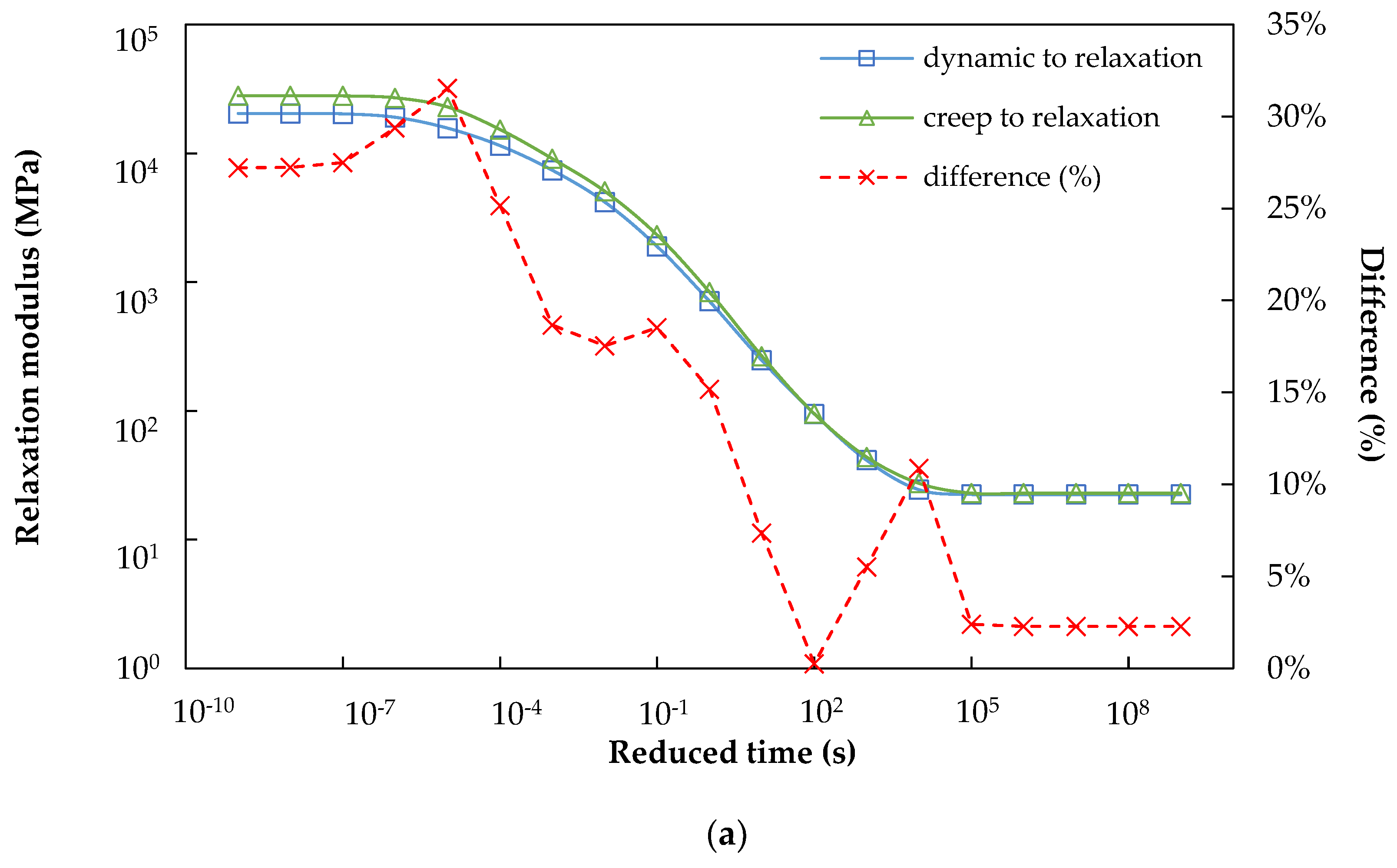
  • The master curves of relaxation modulus converted from dynamic modulus and creep compliance do not present statistical difference at both short- and long-term time domain, and the major difference is observed at the transient time region.
  • Potential reasons for the difference in the transient reduced time region may be attributed to the error in Prony series coefficients. The master curve pattern is sensitive to the Prony series coefficients. However, in the pre-smoothing and fitting process, the approximation is common, leading to loss of information. The most vulnerable time range of relaxation modulus may be the transient reduced time range.

5. Future Studies

The limitation of this paper is that no direct experimental data of relaxation modulus can be acquired to validate the efficiency of these methods. Thus, it cannot be identified which method is more accurate based on the relaxation modulus tests in the premise of same model elements. In future research, the converted relaxation modulus may be integrated into asphalt pavement cracking prediction model to explore its reliability to be the inputs.

Author Contributions

The authors confirm contribution to the paper as follows: study conception and design: W.Z., X.G., B.C.; data collection: W.Z., B.C.; analysis and interpretation of results: B.C., X.G.; draft manuscript preparation: B.C., Q.D. All authors reviewed the results and approved the final version of the manuscript.

Funding

This research was funded by the National Science Foundation of China grant number 51508095, and the Fundamental Research Funds for the Central Universities grant number 2242017K401.

Conflicts of Interest

The authors declare no conflicts of interest.

References

  1. Biot, M.A. Theory of Stress-Strain Relations in Anisotropic Viscoelasticity and Relaxation Phenomena. J. Appl. Phys. 1954, 25, 1385–1391. [Google Scholar] [CrossRef]
  2. Park, S.W.; Kim, Y.R. Interconversion between Relaxation Modulus and Creep Compliance for Viscoelastic Solids. J. Mater. Civ. Eng. 1999, 11, 76–82. [Google Scholar] [CrossRef]
  3. Schapery, R. A Simple Collocation Method for Fitting Viscoelastic Models to Experimental Data; California Institute of Technology: Pasadena, CA, USA, 1962. [Google Scholar]
  4. Mun, S.; Chehab, G.; Kim, Y.R. Determination of Time-domain Viscoelastic Functions using Optimized Interconversion Techniques. Road Mater. Pavement Des. 2007, 8, 351–365. [Google Scholar] [CrossRef]
  5. Kim, Y.R. Modeling of Asphalt Concrete; ASCE Press: Reston, VA, USA, 2009; pp. 751–772. [Google Scholar]
  6. Sun, W.P.; Kim, Y.R.; Schapery, R.A. A viscoelastic continuum damage model and its application to uniaxial behavior of asphalt concrete. Mech. Mater. 1996, 24, 241–255. [Google Scholar]
  7. Williams, M.L. Structural analysis of viscoelastic materials. AIAA J. 2012, 2, 785–808. [Google Scholar] [CrossRef]
  8. Forough, S.A.; Nejad, F.M.; Khodaii, A. Comparing various fitting models to construct the tensile relaxation modulus master curve of asphalt mixes. Int. J. Pavement Eng. 2016, 17, 314–330. [Google Scholar] [CrossRef]
  9. Park, S.W. Analytical modeling of viscoelastic dampers for structural and vibration control. Int. J. Solids Struct. 2001, 38, 8065–8092. [Google Scholar] [CrossRef]
  10. Cost, T.L.; Becker, E.B. A multidata method of approximate Laplace transform inversion. Int. J. Numer. Methods Eng. 1970, 2, 207–219. [Google Scholar] [CrossRef]
  11. Park, S.W.; Kim, Y.R. Fitting Prony-Series Viscoelastic Models with Power-Law Pre-smoothing. J. Mater. Civ. Eng. 2001, 13, 26–32. [Google Scholar] [CrossRef]
  12. Parot, J.M.; Duperray, B. Exact computation of creep compliance and relaxation modulus from complex modulus measurement data. Mech. Mater. 2008, 40, 575–585. [Google Scholar] [CrossRef]
  13. Hu, S.; Zhou, F. Development of a new interconversion tool for hot mix asphalt (HMA) linear viscoelastic functions. Can. J. Civ. Eng. 2010, 37, 1071–1081. [Google Scholar] [CrossRef]
  14. Mun, S.; Zi, G. Modeling the viscoelastic function of asphalt concrete using a spectrum method. Mech. Time-Depend. Mater. 2010, 14, 191–202. [Google Scholar] [CrossRef]
  15. Park, S.W.; Schapery, R.A. Methods of interconversion between linear viscoelastic material functions. Part I—A numerical method based on Prony series. Int. J. Solids Struct. 1999, 36, 1653–1675. [Google Scholar] [CrossRef]
  16. Christensen, R.M.; Freund, L.B. Theory of Viscoelasticity; Academic Press: Cambridge, MA, USA, 1982; p. 720. [Google Scholar]
  17. Denby, E.F. A note on the interconversion of creep, relaxation and recovery. Rheol. Acta 1975, 14, 591–593. [Google Scholar] [CrossRef]
  18. Leaderman, H. Viscoelasticity phenomena in amorphous high polymeric systems. In Rheology; Elsevier Inc.: Amsterdam, The Netherlands, 1958; pp. 1–61. [Google Scholar]
  19. Booij, H.C.; Thoone, G.P.J.M. Generalization of Kramers-Kronig transforms and some approximations of relations between viscoelastic quantities. Rheol. Acta 1982, 21, 15–24. [Google Scholar] [CrossRef]
  20. Schapery, R.A. Approximate Methods of Transform Inversion for Viscoelastic Stress Analysis. Proc. Fourth US Natl. Congr. Appl. Mech. 1962, 2, 1075–1085. [Google Scholar]
  21. Cannone Falchetto, A.; Moon, K.H. Comparisons of analytical and approximate interconversion methods for thermal stress computation. Can. J. Civ. Eng. 2015, 42, 705–719. [Google Scholar] [CrossRef]
  22. Schapery, R.A.; Park, S.W. Methods of interconversion between linear viscoelastic material functions. Part II—An approximate analytical method. Int. J. Solids Struct. 1999, 36, 1677–1699. [Google Scholar] [CrossRef]
  23. Zhao, Y.; Ni, Y.; Zeng, W. A consistent approach for characterising asphalt concrete based on generalised Maxwell or Kelvin model. Road Mater. Pavement Des. 2014, 15, 674–690. [Google Scholar] [CrossRef]
  24. Hopkins, I.L.; Hamming, R.W. On Creep and Relaxation. J. Appl. Phys. 1957, 28, 906–909. [Google Scholar] [CrossRef]
  25. Banks, H.T.; Hu, S.; Kenz, Z.R. A Brief Review of Elasticity and Viscoelasticity for Solids. Adv. Appl. Math. Mech. 2011, 3, 1–51. [Google Scholar] [CrossRef] [Green Version]
  26. Zhang, Y.; Luo, R.; Lytton, R.L. Anisotropic Viscoelastic Properties of Undamaged Asphalt Mixtures. J. Transp. Eng. 2012, 138, 75–89. [Google Scholar] [CrossRef]
  27. Zhao, Y.; Tang, J.; Liu, H. Construction of triaxial dynamic modulus master curve for asphalt mixtures. Constr. Build. Mater. 2012, 37, 21–26. [Google Scholar] [CrossRef]
  28. Forough, S.A.; Nejad, F.M.; Khodaii, A. A comparative study of temperature shifting techniques for construction of relaxation modulus master curve of asphalt mixes. Constr. Build. Mater. 2014, 53, 74–82. [Google Scholar] [CrossRef]
  29. Zhu, H.; Sun, L.; Yang, J.; Chen, Z.; Gu, W. Developing Master Curves and Predicting Dynamic Modulus of Polymer-Modified Asphalt Mixtures. J. Mater. Civ. Eng. 2011, 23, 131–137. [Google Scholar] [CrossRef]
  30. Tarefder, R.A.; Rahman, A.S.M.A. Interconversion of Dynamic Modulus to Creep Compliance and Relaxation Modulus: Numerical Modeling and Laboratory Validation. Presented at the 95th Annual Meeting of the Transport Research Board, Washington, DC, USA, 10–14 January 2016. [Google Scholar]
  31. Tian, X.; Liu, L.; Yu, F.; He, L. Relaxation Modulus Model of Aged Asphalt Mixture. J. Highw. Transp. Res. Dev. 2015, 9, 1–6. [Google Scholar] [CrossRef]
  32. Zhao, Y.; Tang, J.; Long, B. Determination of Relaxation Modulus Using Complex Modulus of Asphalt Mixture. J. Build. Mater. 2012, 15, 498–502. [Google Scholar]
  33. Anderssen, R.S.; Davies, A.R.; de Hoog, F.R. The effect of kernel perturbations when solving the interconversion convolution equation of linear viscoelasticity. Appl. Math. Lett. 2011, 24, 71–75. [Google Scholar] [CrossRef]
  34. Tschoegl, N.W. The Phenomenological Theory of Linear Viscoelastic Behavior; World Publishing Corp.: New York, NY, USA, 1990; pp. 27–29. [Google Scholar]
Figure 1. Mechanical models of viscoelastic materials (a) Generalized Maxwell Model, and (b) Generalized Kelvin Model.
Applsci 08 02447 g001
Figure 2. Master curve fits to experimental data at reference temperature of 21.1 °C for (a) Dynamic modulus; (b) Phase angle.
Applsci 08 02447 g002
Figure 3. Master curve fits to experimental data at reference temperature of 21.1 °C for creep compliance.
Applsci 08 02447 g003
Figure 4. Relaxation modulus master curve converted from creep compliance through collocation method and least squares method in log-log scale.
Applsci 08 02447 g004
Figure 5. Relaxation modulus master curve converted from dynamic modulus and creep compliance (a) in semi-log scale, and (b) in log-log scale.
Applsci 08 02447 g005
Figure 6. Relaxation modulus master curve converted from dynamic modulus and creep compliance in log-log scale for (a) Evotherm; (b) Rubber; (c) Polymer.
Applsci 08 02447 g006aApplsci 08 02447 g006b
Table 1. Aggregate Gradation of Hot Mix Asphalt AC-13.
Sieve Size (mm)1912.59.54.752.361.180.60.30.150.075
Passing Rate (%)10093.074.850.330.324.619.415.010.36.5
Table 2. Summary of fitting parameters for the Hot Mix Asphalt AC-13.
Fitting parameters, dynamic modulus master curve (T0 = 21.1 °C)αβδγ
1.3530 2.8961 0.7631 0.6983
Fitting parameters, phase angle master curve (T0 = 21.1 °C)ξ1ξ2ξ3
−0.6555 −0.0008405−0.59608
Time-temperature shifting factor ( log ( α T ) )4.4 °C21.1 °C37.8 °C54.4 °C
1.8454 0−1.3743 −2.9746
Table 3. Prony Series Coefficients of Relaxation Modulus Obtained from Dynamic Modulus and Creep Compliance.
No. τ j   ( s ) D j   ( 1 / MPa ) ρ i   ( s ) E i   ( MPa )
Dynamic to RelaxationCreep to Relaxation
Collocation MethodLeast Squares
12 × 10−62.14 × 10−62 × 10−62888.601542.072339.76
22 × 10−59.26 × 10−62 × 10−53858.857967.987236.69
32 × 10−42.07 × 10−52 × 10−44791.646962.317381.14
42 × 10−33.91 × 10−52 × 10−34175.536426.106218.63
52 × 10−21.00 × 10−42 × 10−23510.674146.144243.43
62 × 10−12.89 × 10−42 × 10−11669.801712.931750.13
72 × 1008.35 × 10−42 × 100530.77616.41626.74
82 × 1012.63 × 10−32 × 101144.70197.50200.97
92 × 1026.64 × 10−32 × 10242.5664.2767.28
102 × 1031.30 × 10−22 × 10318.2234.1432.71
112 × 1042.92 × 10−22 × 1049.637.638.84
D g   ( 1 / MPa ) 3.33×10⁻⁵ E e   ( MPa ) 21.8318.9418.94
Note: τj and ρi are the relaxation time for creep compliance and dynamic modulus, respectively; Dj is the Prony series for creep compliance.
Table 4. Prony Series Coefficients of Relaxation Modulus Obtained from Dynamic Modulus and Creep Compliance for new data points from previous publications.
No. ρ i   ( s ) E i   ( MPa )
EvothermRubberPolymer
Dynamic to RelaxationCreep to RelaxationDynamic to RelaxationCreep to RelaxationDynamic to RelaxationCreep to Relaxation
12 × 10−62887.791628.272757.412889.772888.432677.87
22 × 10−54120.247975.113796.047164.793842.276895.38
32 × 10−44511.367458.144191.187465.544325.677378.90
42 × 10−33532.574518.683605.385829.683549.115891.67
52 × 10−22838.393347.473139.014460.673207.173560.67
62 × 10−11558.671965.741744.322274.531663.131633.28
72 × 100632.04788.14672.53793.78652.71755.31
82 × 101202.66234.71198.79227.54213.06261.15
92 × 10271.6869.2747.6678.2671.32985.80
102 × 10325.7622.5039.7642.7130.2939.23
112 × 1043.017.098.329.456.9011.19
E e   ( MPa ) 22.3822.9023.1523.6623.1425.46

