Retrieval of Similar Evolution Patterns from Satellite Image Time Series ^†

Abstract

Technological evolution in the remote sensing domain has allowed the acquisition of large archives of satellite image time series (SITS) for Earth Observation. In this context, the need to interpret Earth Observation image time series is continuously increasing and the extraction of information from these archives has become difficult without adequate tools. In this paper, we propose a fast and effective two-step technique for the retrieval of spatio-temporal patterns that are similar to a given query. The method is based on a query-by-example procedure whose inputs are evolution patterns provided by the end-user and outputs are other similar spatio-temporal patterns. The comparison between the temporal sequences and the queries is performed using the Dynamic Time Warping alignment method, whereas the separation between similar and non-similar patterns is determined via Expectation-Maximization. The experiments, which are assessed on both short and long SITS, prove the effectiveness of the proposed SITS retrieval method for different application scenarios. For the short SITS, we considered two application scenarios, namely the construction of two accumulation lakes and flooding caused by heavy rain. For the long SITS, we used a database formed of 88 Landsat images, and we showed that the proposed method is able to retrieve similar patterns of land cover and land use.

1. Introduction

Over the years, the remote sensing domain has been characterized by numerous technological improvements (e.g., increased spatial resolution, shorter revisit time, increased number of spectral bands). These improvements were made possible through several Earth Observation missions, e.g., the Landsat program sustained by NASA and the United Stated Geological Survey (USGS), the Sentinel program financed by European Space Agency, Envisat’s ASAR mission. In addition, many of the recent missions have functioned under an open data access policy for research purposes. This fact has a direct impact on the interest manifested in using this type of data in many realms, such as agriculture, land cover and land use planning, resource management, urbanization, and sustainable development.

One possible method for the analysis of satellite image time series (SITS) is to compare two satellite images captured at two successive moments of time, over the same area of interest [1,2,3,4]. These methods are generally called change detection methods. However, although they can successfully detect abrupt changes (e.g., deforestation, natural disasters, building construction), these methods are not able to identify complex spatio-temporal structures that evolve in a defined time-frame (e.g., measuring the effects of floods, urban expansion, land cover and land use modifications). In the later cases, SITS analysis methods that involve information extraction from multi-temporal data are usually preferred.

The main difficulties when dealing with SITS are the irregular time sampling, the missing samples (e.g., due to cloud cluttering and haze that affect images captured by optical sensors, technical artifacts) and, also, the high spatial and temporal data dimensionality. In general, multi-temporal approaches require the processing of large amounts of data characterized by a high degree of variability in terms of temporal, spatial and multi-spectral information.

The spatio-temporal evolution patterns may span different periods of time and may affect small to large regions. For example, urban transformations affect small regions and have multiple construction phases spanning several years. In contrast, flood events may affect larger areas then in the previous case, but, depending on their intensity, the consequences may be observed over shorter or longer periods of time (e.g., land slides are irreversible). In this context, the characterization of temporal evolutions is strictly related to the fact that the processes that occur in dynamic scenes have different time scales and affect small to large areas.

Therefore, the requirements that SITS analysis methods must fulfill are: (1) the ability to capture complex spatio-temporal changes and (2) the potential to emphasize both short-term and long-term modifications. Developing an algorithm that can deal with the spatial, temporal and spectral diversity of Earth Observation data is a challenging task to accomplish and more so when the amount of knowledge that a human expert transfers to the system is limited.

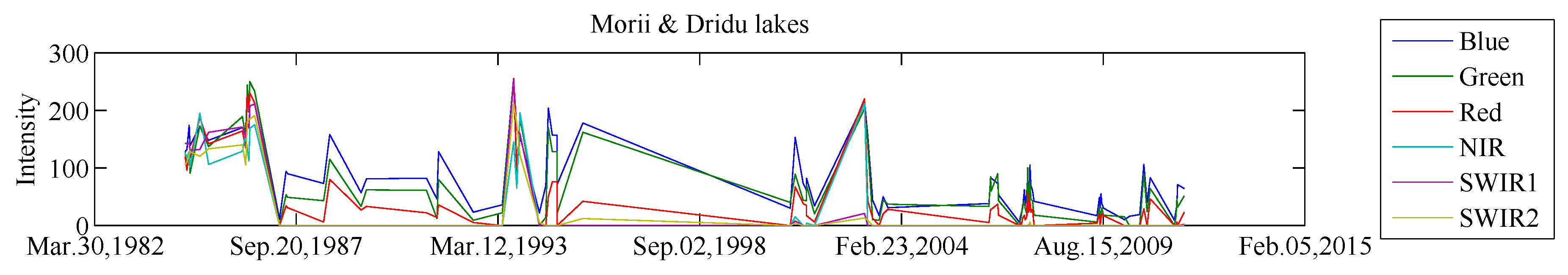
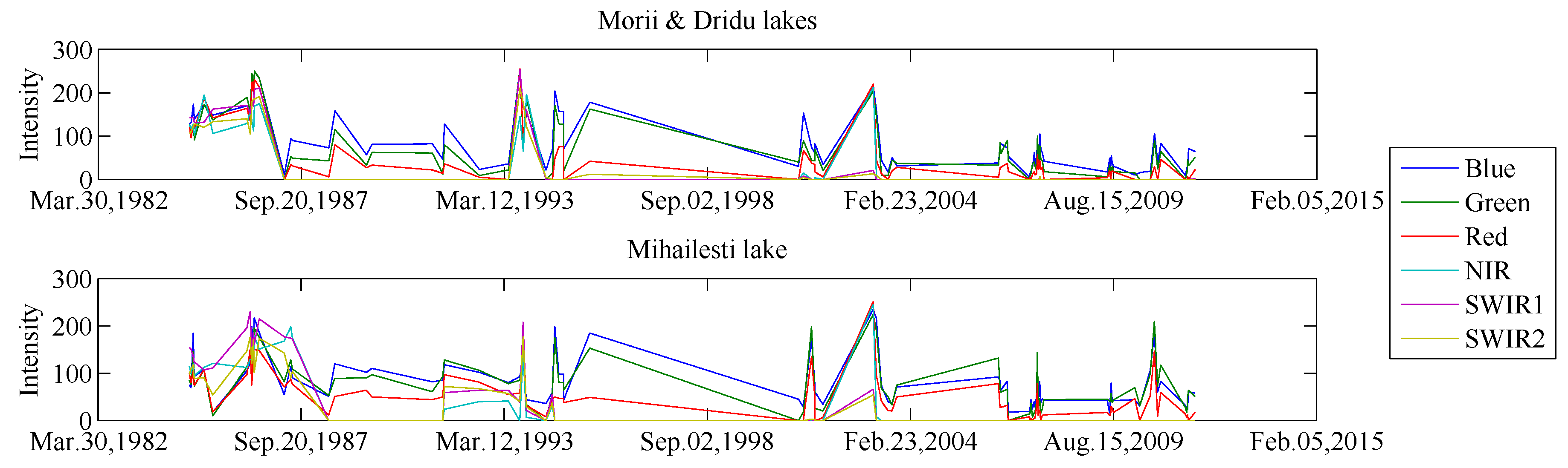
Many multi-temporal analysis techniques use a SITS classification that incorporates various dissimilarity measures to compare two temporal sequences. In SITS, by similar evolution, we understand a group of scene points that share the same behavior for the entire period of time or for most of it. Each point in a SITS is characterized by a spectro-temporal signature. An example of a spectro-temporal signature is provided in Figure 1 for a SITS acquired by the Landsat sensor with six spectral bands.

Some of the methods used to assess the degree of similarity between temporal sequences have emerged directly from text classification, speech recognition, or genomic data classification [5,6]. Dynamic Time Warping (DTW) has proved to be an essential tool not only for spoken-word recognition, but also for understanding similarities between evolution profiles in SITS [7,8]. DTW is able of handling comparisons between sequences characterized by irregular time sampling or missing data issues [7]. In this regard, K-means with DTW as the distance measure the yield land cover and land use maps of SITS [7]. However, performing an unsupervised clustering over an entire multi-spectral SITS data is time-consuming, and the temporal characteristics of the data may be missed. Other versions of DTW include a weighting procedure to mark the seasonality characteristics of temporal evolutions [9,10]. This weighting procedure works well for cropland mapping, but it may not be helpful for other applications that do not account for a periodicity effect (e.g., construction of buildings). In addition, recently, a tree-based structure formed of multiple K-means clustering algorithms that use the DTW distance measure was developed in [11] for the indexing and classification of SITS.

The methodology described in [12] for time series analysis is based on computing change maps between pairs of consecutive images using different similarity measures (e.g., correlation coefficient, first order Kullback–Liebler Divergence, Conditional Information, Normalized Compression Distance). The change maps are transformed into a collection of words through the K-means clustering algorithm. All the words form a dictionary. The transformed change maps are processed afterwards using the Latent Dirichlet Allocation (LDA) model to discover classes (or evolution-topics) based on the latent information from the scene. Thus, the final results of the analysis provide an unsupervised classification of the spatio-temporal evolutions into classes.

A study of several general purpose supervised classifiers, like Random Forest and Support Vector Machine (SVM), was presented in [13] as a solution for land cover mapping. The features extracted from the images were spectral features (e.g., color, normalized difference vegetation, water and build-up indexes, brightness, greenness, wetness, brilliance) and temporal features (e.g., statistical values from normalized difference vegetation index profile, phenological parameters marking important events in a season like sowing, threshing, cropping). However, SVM and Random Forest classifiers are known for having large training times, which may last even several days [13]. In this sense, this type of classification system cannot be used for online retrieval of spatio-temporal evolutions, where a fast response is needed. In addition, supervised classifiers need large amounts of training data. This requirement is not easy to fulfill in SITS classification tasks.

Frequent sequential pattern analysis was introduced in [14,15] for unsupervised SITS mining. This approach performs a quantization of the images in the SITS using a fixed number of gray levels (or, labels) and forms a sequence of T labels for each pixel location, where T is the number of images in the SITS. In this context, an ordered list of labels is called a frequent sequential pattern if the number of its occurrences in the SITS is greater than a fixed threshold. Inferring spatial connectivity constraints when determining the frequent sequential patterns proved to be efficient in monitoring crop or ground deformations [14]. However, the determination of the frequency of sequential patterns in SITS is sensitive to the number of levels used for image quantization. In addition, the method extracts a large number of patterns which may be difficult to interpret in terms of changes that appear in an area. Moreover, missing data may raise difficulties when interpreting the results for SITS analysis.

Apart from the irregular time sampling, missing data, and high data variability in the spatial, temporal, and spectral domains that were mentioned above, another difficult challenge that is met in SITS analysis is the assignment of semantic meaning to patterns of spatio-temporal evolution. This challenge is most frequently met when unsupervised techniques are used for SITS analysis. In these cases, a method to determine the optimal number of evolution classes is usually used [16]. A query-by-example retrieval method would alleviate this issue by associating semantic meaning to each query that a user addresses to the retrieval system. In this regard, we hereby present a query-by-example retrieval method whose goal is to separate spatio-temporal evolutions that are similar to a given query from non-similar ones. After the user performs a specific query, the retrieval method consists of two main steps. Firstly, the system performs the computation of distance measures between the query and the rest of spatio-temporal evolutions. Secondly, an optimal threshold is determined through the Expectation-Maximization technique in order to obtain a binary map displaying similar patterns with respect to the given query. The rest of the paper is structured as follows. The two-step retrieval method is presented in Section 2. Section 3 and Section 4 present the experiments conducted over several SITS datasets, discuss the results obtained for different application scenarios, and compare the proposed method to other SITS analysis methods. Finally, the last section concludes the paper.

2. Materials and Methods

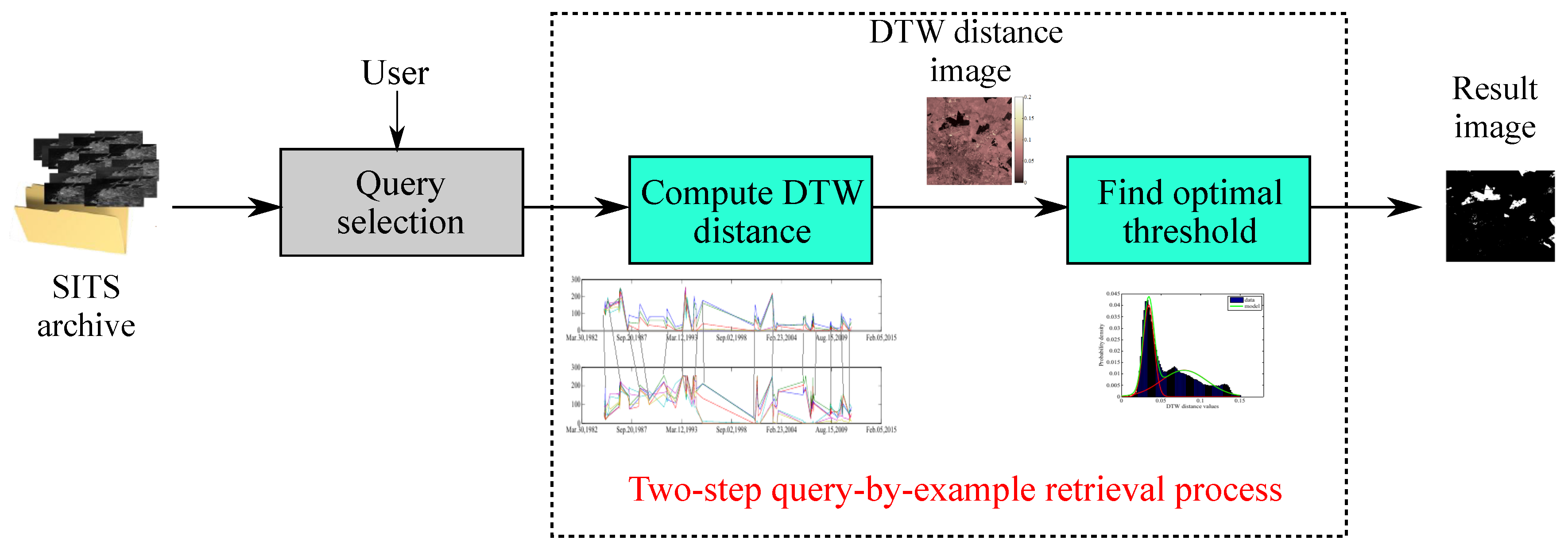
In this paper, the SITS analysis is approached through time series information retrieval, which is the process of searching inside a collection of data. The proposed search process starts with a query provided by the end-user, whose aim is to identify evolutions that are similar (i.e., have similar behavior) to the selected query. Firstly, the proposed method determines the degree of similarity between a specific query and the rest of the spatio-temporal evolutions. This step is performed by computing the DTW measure between the query and the rest of the evolutions. The DTW score is expected to be small for similar evolutions and large for non-similar ones. The retrieval process consists of deciding whether a certain evolution is similar to the given query or not. In this sense, the retrieval process can be seen as a problem of separating the spatio-temporal evolutions into two classes (i.e., similar versus non-similar with respect to a given query). The class identification is performed via Bayesian decision theory and it is based on determining the optimal threshold that separates relevant from irrelevant evolution patterns with respect to a given query.

Specifically, the proposed approach is a two-step process: (1) compute DTW distances and (2) find the optimal threshold. The process is summarized in Figure 2 and starts by computing a DTW distance image containing all the DTW dissimilarity scores with respect to a fixed query. After applying the optimal threshold over the DTW distance image, the final result is a binary map which aids in delimiting similar spatio-temporal evolutions.

2.1. Dynamic Time Warping (DTW)

The first step in retrieving spatio-temporal patterns that are similar to a given query is to measure the degree of similarity between the query sequence and the rest of the sequences. This can be achieved through Dynamic Time Warping, which has been widely used in many applications related to speech recognition [5] and DNA analysis [6]. The method is usually applied to find the optimal alignment path between two sequences, $U_1^T=({\mathbf{u}}_1,\dots ,{\mathbf{u}}_T)$ and $V_1^{T^{\prime }}=({\mathbf{v}}_1,\dots ,{\mathbf{v}}_{T^{\prime }})$, which may have different lengths (i.e., $T\ne T^{\prime }$) [17]. This is a frequently met situation in SITS analysis due to technological artifacts or cloud cluttering problems that may occur in images captured by optical remote sensing sensors. Mathematically, the DTW distance measure between two sequences, $U_1^i=({\mathbf{u}}_1,\dots ,{\mathbf{u}}_i)$ and $V_1^j=({\mathbf{v}}_1,\dots ,{\mathbf{v}}_j)$, can be recurrently defined as

$$D_{i,j}=\delta ({\mathbf{u}}_i,{\mathbf{v}}_j)+min(D_{i-1,j-1},D_{i-1,j},D_{i,j-1})$$

(1)

where $\delta$ is the Euclidean distance between two current elements ${\mathbf{u}}_i$ and ${\mathbf{v}}_j$ of the sequences, $D_{k,l}$ is the partial similarity score between $U_1^k$ and $V_1^l$ for any $k\le T$ and $l\le T^{\prime }$. As can be observed from the above equation, the optimization problem aims at finding the best alignment between subsequences of $U_1^T$ and $V_1^{T^{\prime }}$.

In the above formulation, the following initial conditions are considered:

$$\begin{array}{cc}\hfill D_{1,1}& =\delta ({\mathbf{u}}_1,{\mathbf{v}}_1)\hfill \end{array}$$

(2)

$$\begin{array}{cc}\hfill D_{1,j}& =\sum _{p=1}^j\delta ({\mathbf{u}}_1,{\mathbf{v}}_p)\hfill \end{array}$$

(3)

$$\begin{array}{cc}\hfill D_{i,1}& =\sum _{q=1}^i\delta ({\mathbf{u}}_q,{\mathbf{v}}_1).\hfill \end{array}$$

(4)

The overall DTW similarity between $U_1^T$ and $V_1^{T^{\prime }}$ is given by the score $D_{T,T^{\prime }}$. Computing the overall score is equivalent to determining the elements of a $T\times T^{\prime }$ distance matrix where the element on row i and column j is $D_{i,j}$.

The recurrence relation used in the computation of the DTW similarity score implies the computation of a $T\times T^{\prime }$ matrix, whose elements are the distances $D_{i,j}$ ($1\le i\le T$, $1\le j\le T^{\prime }$). Each distance $D_{i,j}$ uses the smallest value between the closest previous neighbors in the matrix. The DTW matrix is computed from left to right and top to bottom. The last element $D_{T,T^{\prime }}$ represents the overall DTW score of similarity, whilst the path that is followed to compute the score of similarity provides the optimal alignment. An example of DTW-based optimal alignment together with the DTW distance matrix D is shown in

Table 1. Example of computation of the Dynamic Time Warping (DTW) distance matrix for two sequences, ’5463545’ and ’0102130’.

	0	1	0	2	1	3	0
5	5	9	14	17	21	23	28
4	9	8	12	14	17	18	22
6	15	13	14	16	19	20	24
3	18	15	16	15	16	16	19
5	23	19	20	18	20	18	21
4	27	22	23	20	21	19	22
5	32	26	27	23	24	21	24

for two sequences of one-dimensional elements. In this example, we considered that $\delta$ is the difference in absolute values of the elements. The element on the lower-right of the matrix is the total score of the similarity between the two sequences.

If the similarity scores are computed between spatio-temporal sequences in a multispectral SITS, the sequences are formed by the vector elements ${\mathbf{u}}_i$ and ${\mathbf{v}}_j$ whose dimensions are given by the number of frequency bands used by the remote sensing sensors. Let us denote by c the number of spectral bands. Then, $\delta$ is the Euclidean distance between two vector elements in a space with c dimensions:

$$\delta ({\mathbf{u}}_i,{\mathbf{v}}_j)=\sqrt{\sum _{k=1}^c{(u_{i,k}-v_{j,k})}^2}$$

(5)

where ${\mathbf{u}}_i={[u_{i,1},\dots ,u_{i,c}]}^T$ and ${\mathbf{v}}_j={[v_{j,1},\dots ,v_{j,c}]}^T$.

The DTW similarity score is computed between the query provided by the user and each spatio-temporal sequence in the SITS. The result is a DTW distance image $\mathbf{DI}$ that assesses the scores of similarity between the given query and the evolutions for each pixel location.

As already mentioned, the DTW distance is expected to be small for evolutions that are similar to the query and large for non-similar evolutions. This is due to the fact that, if the spatio-temporal evolutions are similar, the DTW algorithm finds an alignment with a smaller cost between the corresponding temporal sequences and the given query than in the case of non-similar evolutions. Therefore, the separation of similar from non-similar evolution patterns is equivalent to finding an optimal threshold that can be applied over DTW distances in order to retrieve the specific pattern queried by the end-user.

2.2. Determining the Optimal Threshold Using Expectation-Maximization

In the previous subsection, we described the process of determining the DTW distance image $\mathbf{DI}$ containing DTW similarity scores with respect to a query selected by an end-user. The following step in the automatic extraction of evolutions that have similar behavior to a given query is the optimal thresholding step. More precisely, we aim to separate the DTW distance scores between two classes, a class of similar evolutions and a class of non-similar spatio-temporal evolutions. Separating these two classes of evolutions translates into finding the optimal threshold to be applied on the DTW similarity scores. In this sense, we formulate the problem of query-by-example SITS retrieval in terms of the Bayesian decision theory.

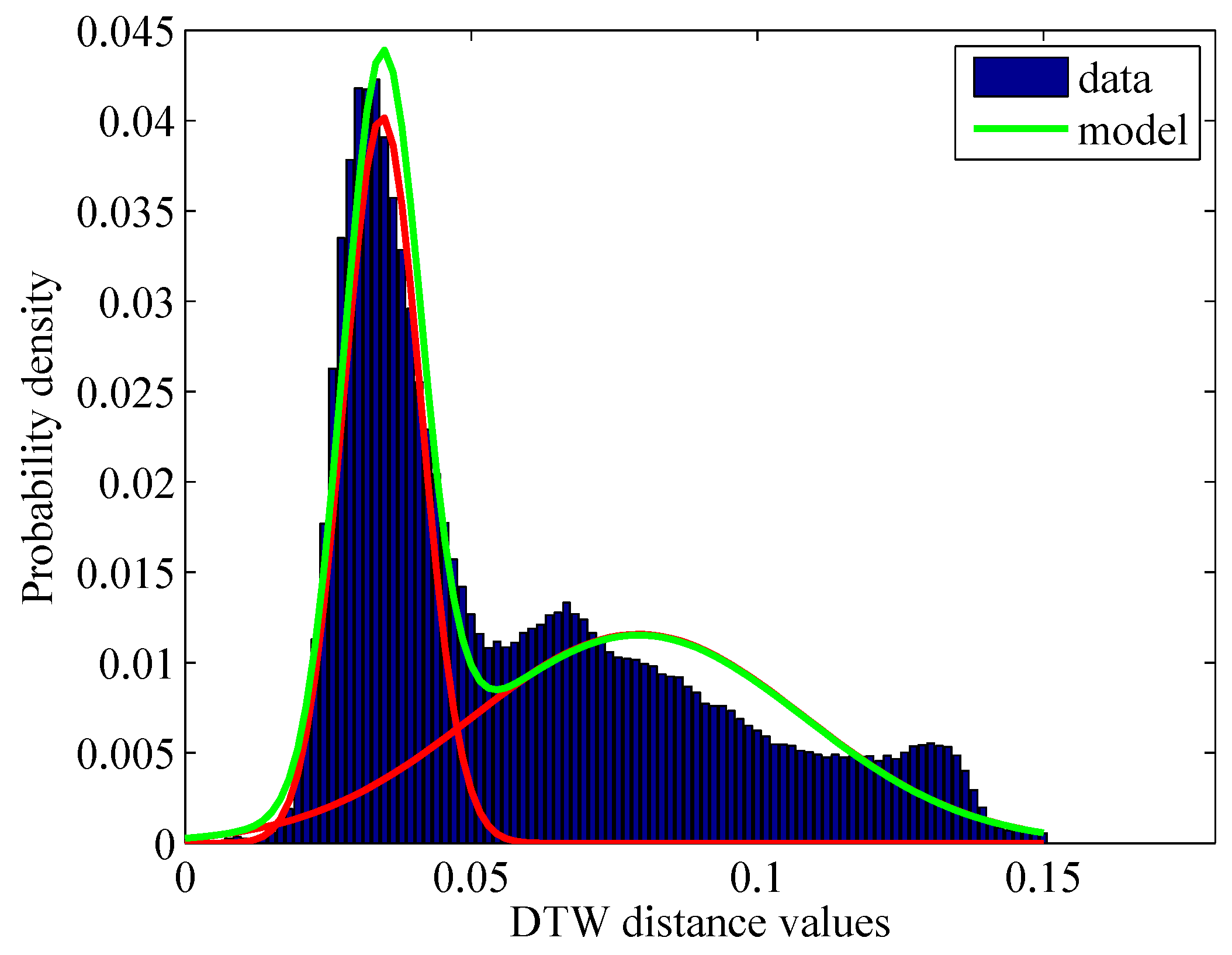
The DTW similarity scores computed for a given query follow a multimodal distribution. This can be observed from Figure 3, where the query selected for retrieval is from an agricultural area in a long SITS (88 temporal samples). As expected, the first lobe corresponds to similar evolutions. This is argued by the fact that DTW similarity scores are smaller for similar evolutions than for non-similar evolutions. Furthermore, the histogram profile shown in Figure 3 confirms the idea of separating similar from non-similar evolutions using the Maximum Likelihood (ML) technique.

In the following text, we denote the random variable associated to the computed DTW similarity scores by X, whilst x represents a particular DTW score. Following the formalism initially presented in [18], let us assume that the scores are drawn from a mixture of two Gaussian distributions, $\mathcal{N}({\mu }_s,{\sigma }_s)$ and $\mathcal{N}({\mu }_n,{\sigma }_n)$. The first Gaussian distribution corresponds to evolutions that are similar to the given query, whereas the second component refers to non-similar evolutions.

The Maximum Likelihood Estimation (MLE) framework determines the parameter values that make the observed data most likely, i.e., that maximize the likelihood function and fit the model to the data. Following the above considerations, the overall posterior probability can be decomposed as

$$p_{\theta }\left(x\right)={\pi }_s\mathcal{N}\left(x\right|{\mu }_s,{\sigma }_s)+{\pi }_n\mathcal{N}\left(x\right|{\mu }_n,{\sigma }_n)$$

(6)

where $\theta =\left\{{\pi }_s,{\mu }_s,{\sigma }_s,{\pi }_n,{\mu }_n,{\sigma }_n\right\}$ is the set of model parameters, whilst ${\pi }_s$ and ${\pi }_n$ are the mixture probabilities [19] such that ${\pi }_s+{\pi }_n=1$. The mixture components are modeled as Gaussian densities:

$$\mathcal{N}\left(x\right|{\mu }_k,{\sigma }_k)=\frac{1}{\sqrt{2\pi {\sigma }_k^2}}exp\left[-\frac{{(x-{\mu }_k)}^2}{2{\sigma }_k^2}\right]$$

(7)

with $k\in \{s,n\}$, whilst $({\mu }_s,{\sigma }_s)$ and $({\mu }_n,{\sigma }_n)$ are the mean and standard deviation pairs corresponding to similar and non-similar evolutions, respectively. The set of parameters $\theta$ is determined iteratively using the Expectation-Maximization (EM) algorithm. Specifically, each iteration j is decomposed in two basic steps:

• Expectation step (E-step). Compute the log-likelihood (i.e., the logarithm of the posterior probability) with respect to the current values of the parameters ${\theta }^{\left(t\right)}$:

  $$L\left({\theta }^{\left(t\right)}\right)=ln{p}_{{\theta }^{\left(t\right)}}\left(x\right)$$

  (8)
• Maximization step (M-step). Update the model parameters such that the log-likelihood approaches its maximum, i.e., the convergence of the EM algorithm guarantees that the log-likelihood value is increased with each iteration [19]. It is usually convenient to introduce a mapping between the new model parameters ${\theta }^{(t+1)}$ and the previous ones ${\theta }^{\left(t\right)}$. According to [18] and following the notations in [19], the means, squared standard deviations, and mixture probabilities for each class $k\in \{s,n\}$ can be re-estimated using the following set of relations:

  $$\begin{array}{ccc}\hfill {\pi }_k^{(t+1)}& =& \frac{{\displaystyle \sum _x}{\zeta }_k^{\left(t\right)}\left(x\right)}{N}\hfill \end{array}$$

  (9)

  $$\begin{array}{ccc}\hfill {\mu }_k^{(t+1)}& =& \frac{{\displaystyle \sum _x}{\zeta }_k^{\left(t\right)}\left(x\right)·x}{{\displaystyle \sum _x}{\zeta }_k^{\left(t\right)}\left(x\right)}\hfill \end{array}$$

  (10)

  $$\begin{array}{ccc}\hfill {\sigma }_k^{(t+1)}& =& {\left(\frac{{\displaystyle \sum _x}{\zeta }_k^{\left(t\right)}\left(x\right)·{\left(x-{\mu }_k^{\left(t\right)}\right)}^2}{{\displaystyle \sum _x}{\zeta }_k^{\left(t\right)}\left(x\right)}\right)}^{\frac{1}{2}}\hfill \end{array}$$

  (11)

  where $N=W\times H$ is the total number of pixels in the distance image (i.e., the number of spatio-temporal evolutions) and ${\zeta }_k^{\left(t\right)}\left(x\right)$ values are derived as

  $${\zeta }_k^{\left(t\right)}\left(x\right)=\frac{{\pi }_k^{\left(t\right)}\mathcal{N}\left(x\right|{\mu }_k^{\left(t\right)},{\sigma }_k^{\left(t\right)})}{{\sum }_{k^{\prime }}{\pi }_{k^{\prime }}^{\left(t\right)}\mathcal{N}\left(x\right|{\mu }_{k^{\prime }}^{\left(t\right)},{\sigma }_{k^{\prime }}^{\left(t\right)})}.$$

  (12)

The initialization of the EM algorithm is done by separating the similarity scores into two subsets, ${\mathcal{S}}_n^{\left(0\right)}$ and ${\mathcal{S}}_c^{\left(0\right)}$. Any unsupervised clustering method can be applied, but we chose the K-means ($K=2$) clustering method due to its fast response time when the number of clusters is small. However, being an unsupervised clustering method, a constraint must still be fulfilled. Namely, the cluster of similar evolutions must be characterized by DTW similarity scores that are smaller than the DTW similarity scores obtained for the temporal sequences pertaining to the cluster of non-similar evolutions with respect to the query. The initial values for the prior probabilities, means, and squared standard deviations can be easily computed as statistics over the two subsets, ${\mathcal{S}}_n^{\left(0\right)}$ and ${\mathcal{S}}_c^{\left(0\right)}$. Compared to the initialization proposed in [1], the K-means initialization speeds up the convergence of the EM algorithm [19], and thus, the speed of the whole algorithm.

After the estimation of the $\theta$ model parameters, the optimal threshold $T_o$ that separates the two classes (i.e., similar and non-similar) is determined from the equality

$${\pi }_s\mathcal{N}\left(T_o\right|{\mu }_s,{\sigma }_s)={\pi }_n\mathcal{N}\left(T_o\right|{\mu }_n,{\sigma }_n)$$

(13)

that naturally follows from the Maximum Likelihood rule

$${\pi }_s\mathcal{N}\left(x\right|{\mu }_s,{\sigma }_s)\underset{n}{\stackrel{s}{\gtrless }}{\pi }_n\mathcal{N}\left(x\right|{\mu }_n,{\sigma }_n).$$

(14)

Taking the logarithm of both sides of Equation (13) yields a quadratic equation in $T_o$

$$({\sigma }_n^2-{\sigma }_s^2)T_o^2+2\left({\mu }_n{\sigma }_s^2-{\mu }_s{\sigma }_n^2\right)T_o+{\mu }_s^2{\sigma }_n^2-{\mu }_n^2{\sigma }_s^2-2{\sigma }_s^2{\sigma }_n^{2}ln\left[\frac{{\sigma }_n{\pi }_s}{{\sigma }_s{\pi }_n}\right]=0$$

(15)

that has two possible solutions. However, only one of these solutions lies between ${\mu }_s$ and ${\mu }_n$ and this solution represents the optimal threshold value.

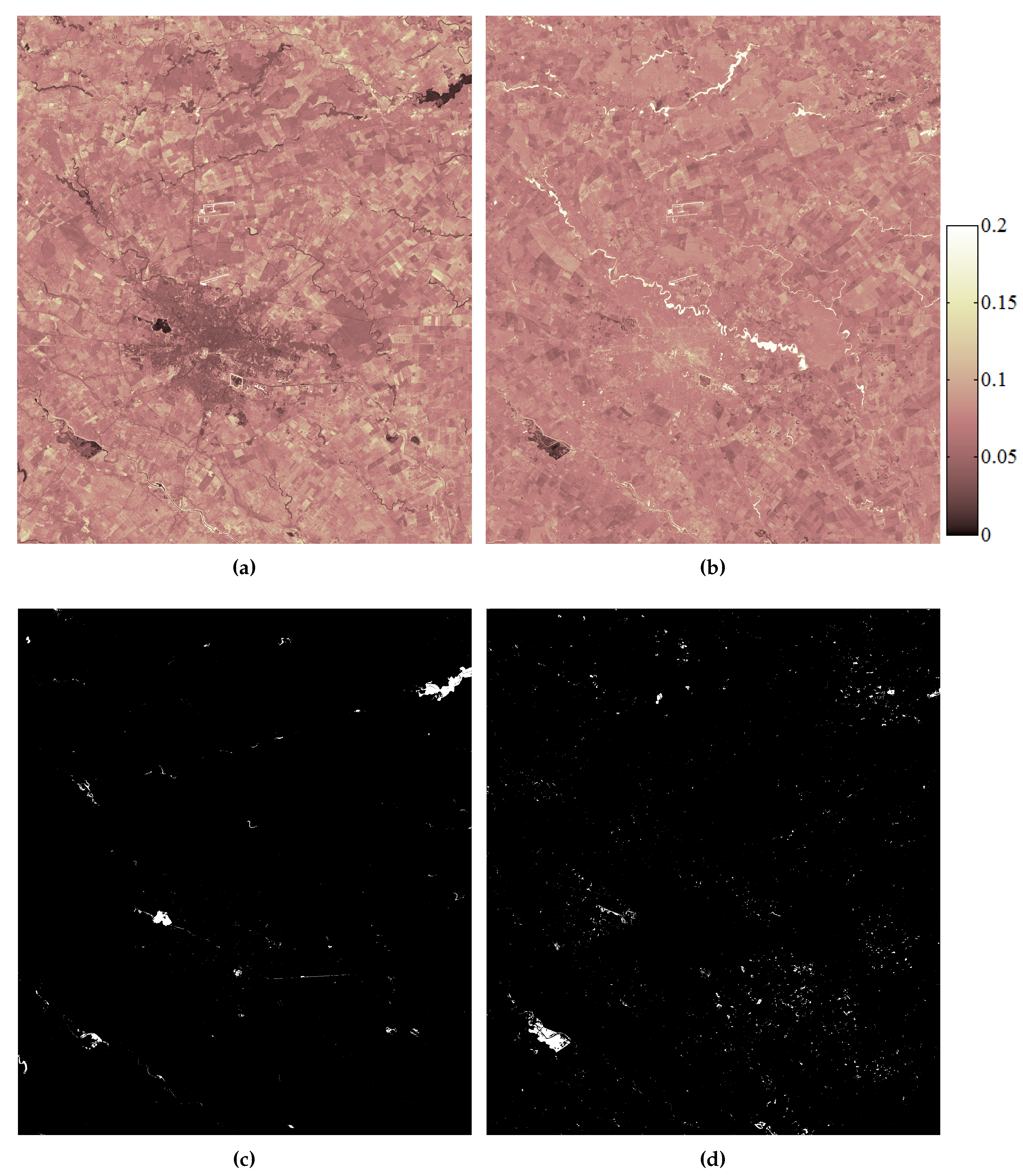
After determining the optimal threshold value $T_o$, the DTW distance image $\mathbf{DI}$ is transformed into a binary image $\mathbf{S}$, delimiting the locations of evolutions that are similar to the given query:

$$\mathbf{S}(w,h)=\left\{\begin{array}{c}1,\mathbf{DI}(w,h)\le T_o\hfill \\ 0,\mathrm{otherwise}\hfill \end{array}\right.$$

(16)

where $1\le w\le W$ and $1\le h\le H$, W and H being the width and height of the images in SITS.

3. Experiments

The proposed method for the retrieval of specific spatio-temporal patterns in SITS was tested on series of Landsat images captured at different periods of time and over different locations. In all application scenarios described hereafter, all of the available spectral bands were taken into consideration, namely green, red, blue, Near Infrared and two Short-Wave Infrared bands. Moreover, the spatial resolution of the Landsat sensor was 30 m.

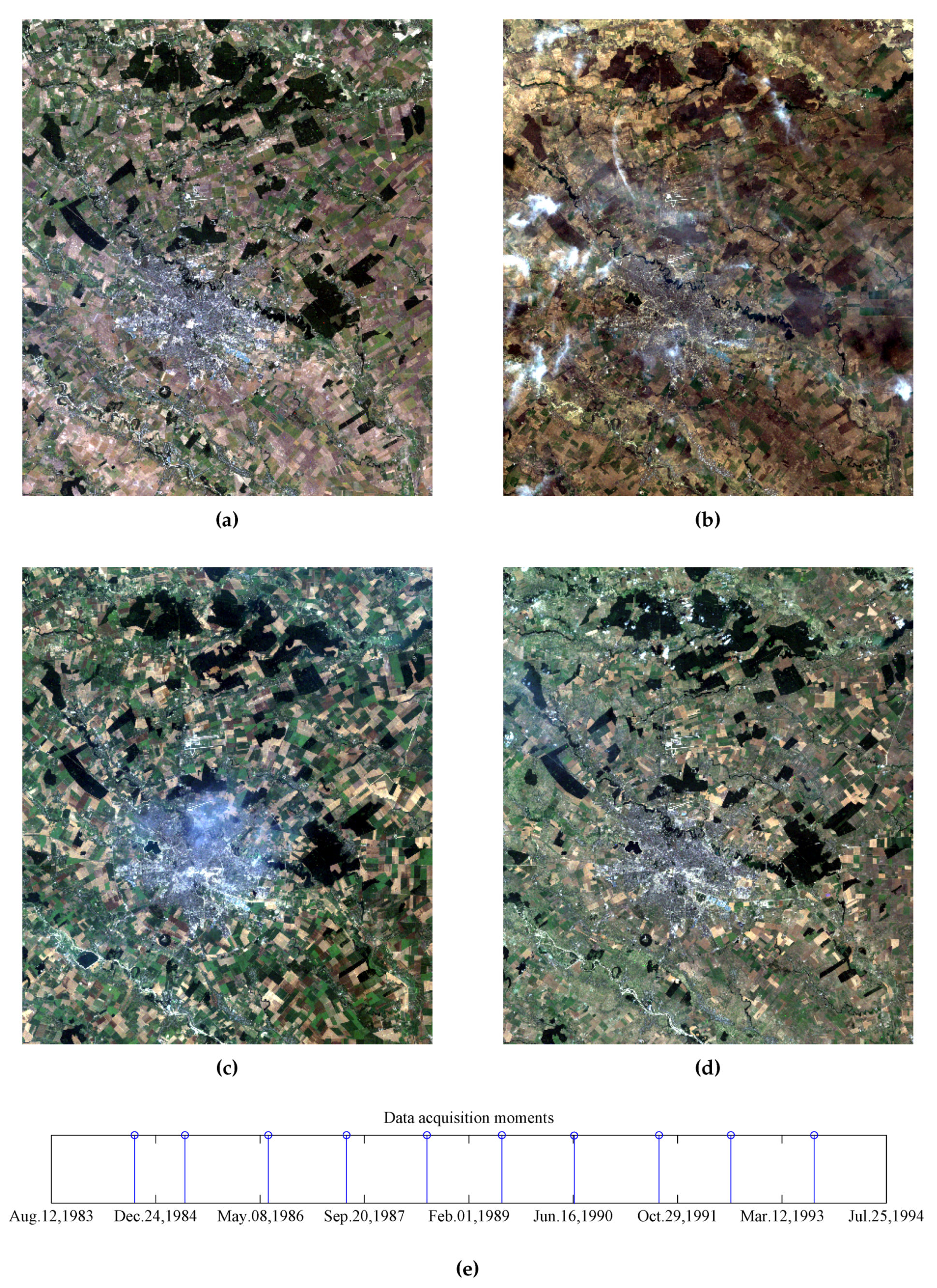
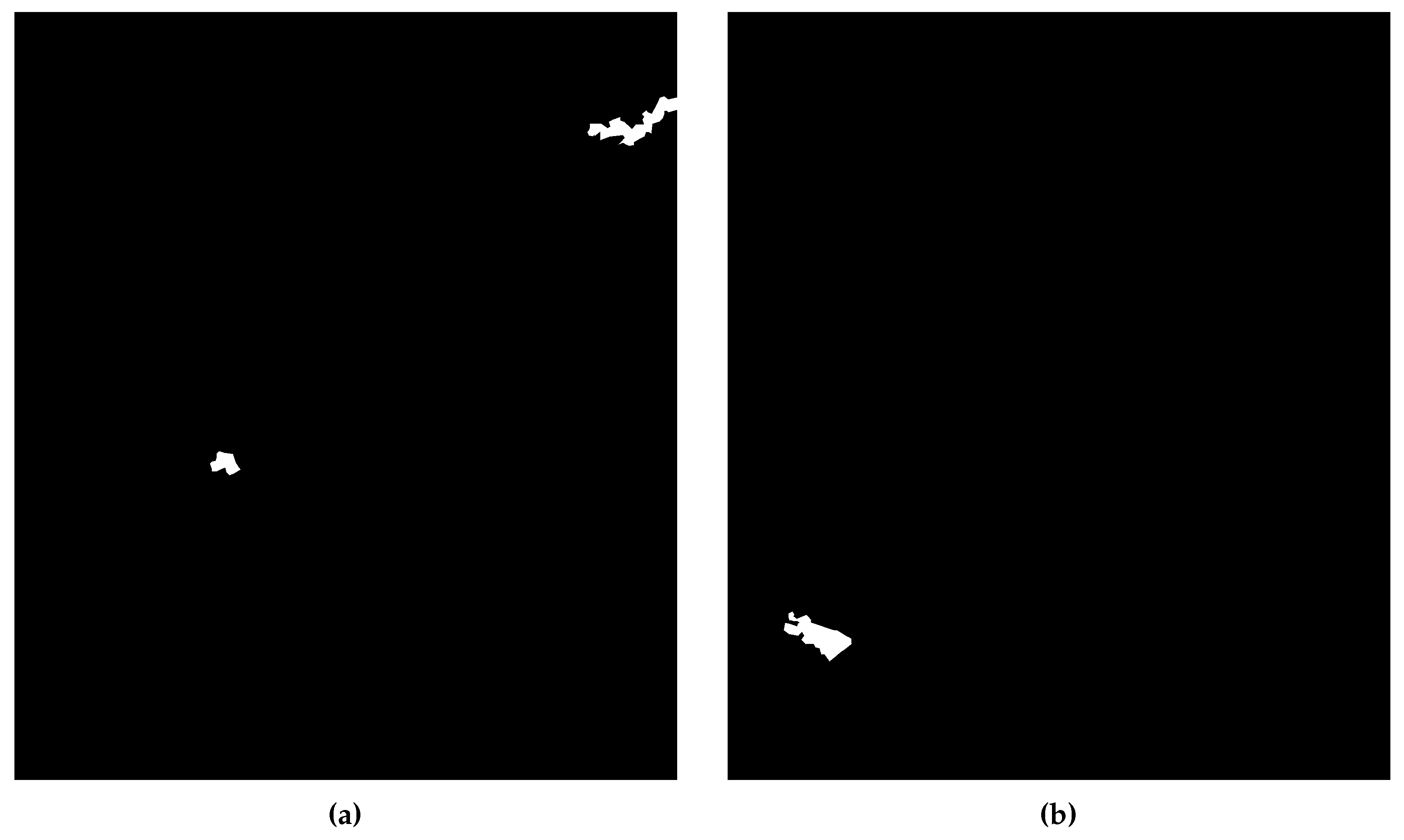
The first series consists of a short time series of 10 images acquired between 1984 and 1993 (i.e., an image is acquired each year), over Bucharest, Romania, and regions surrounding the city. The size of the images is $1702\times 1975$ pixels and the captures were taken in different seasons of the years. Several samples of the time series, along with their acquisition moments, are shown in Figure 4. In this case, the task was to determine similar changes that occurred during the formation of three accumulation lakes near Bucharest, namely Dridu, Mihailesti, and Morii. Two of these lakes evolved similarly, whereas the third one went through several modifications over the time period mentioned above.

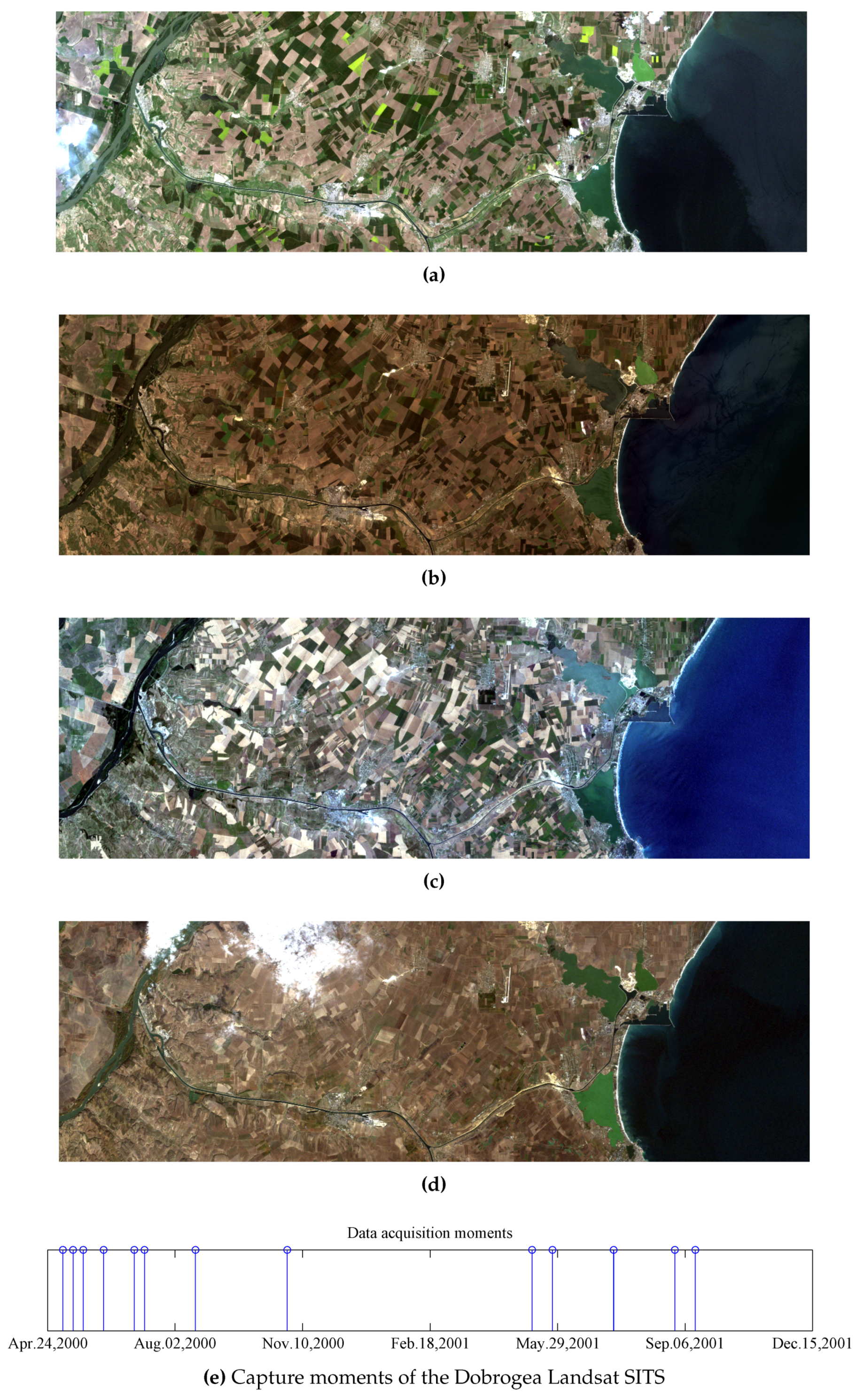
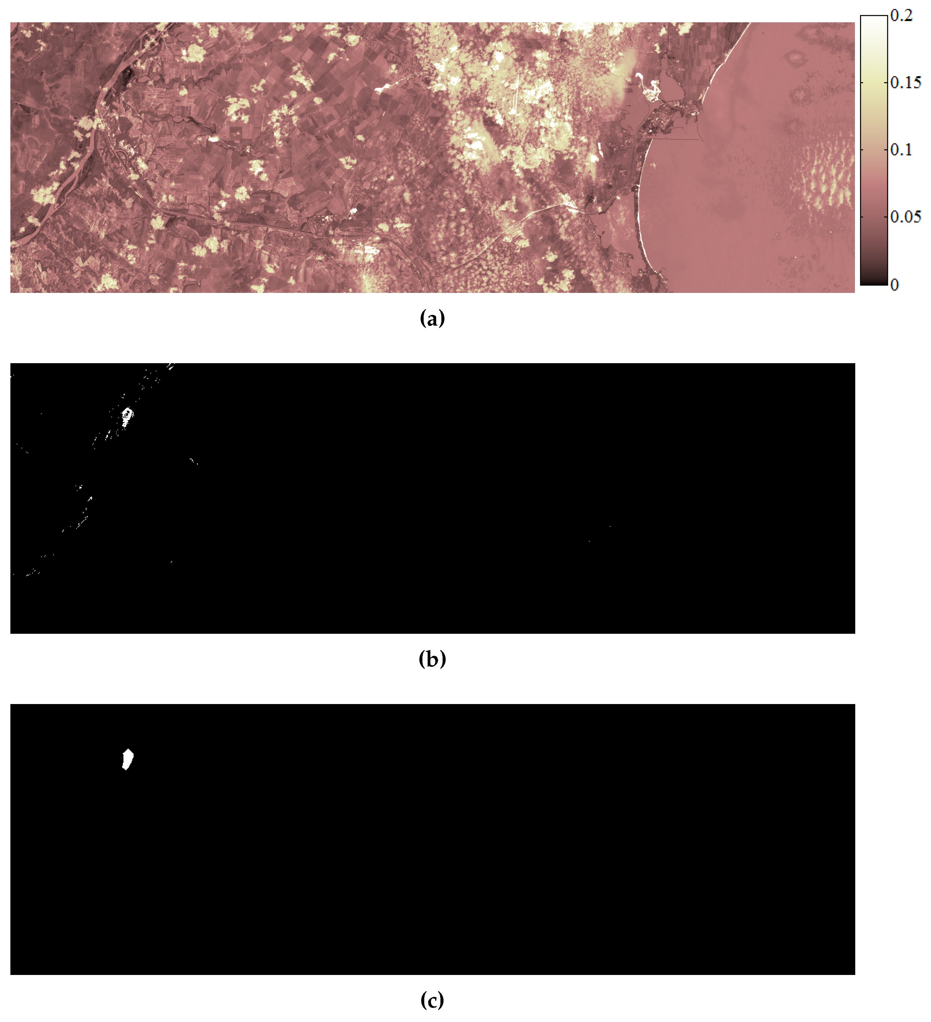
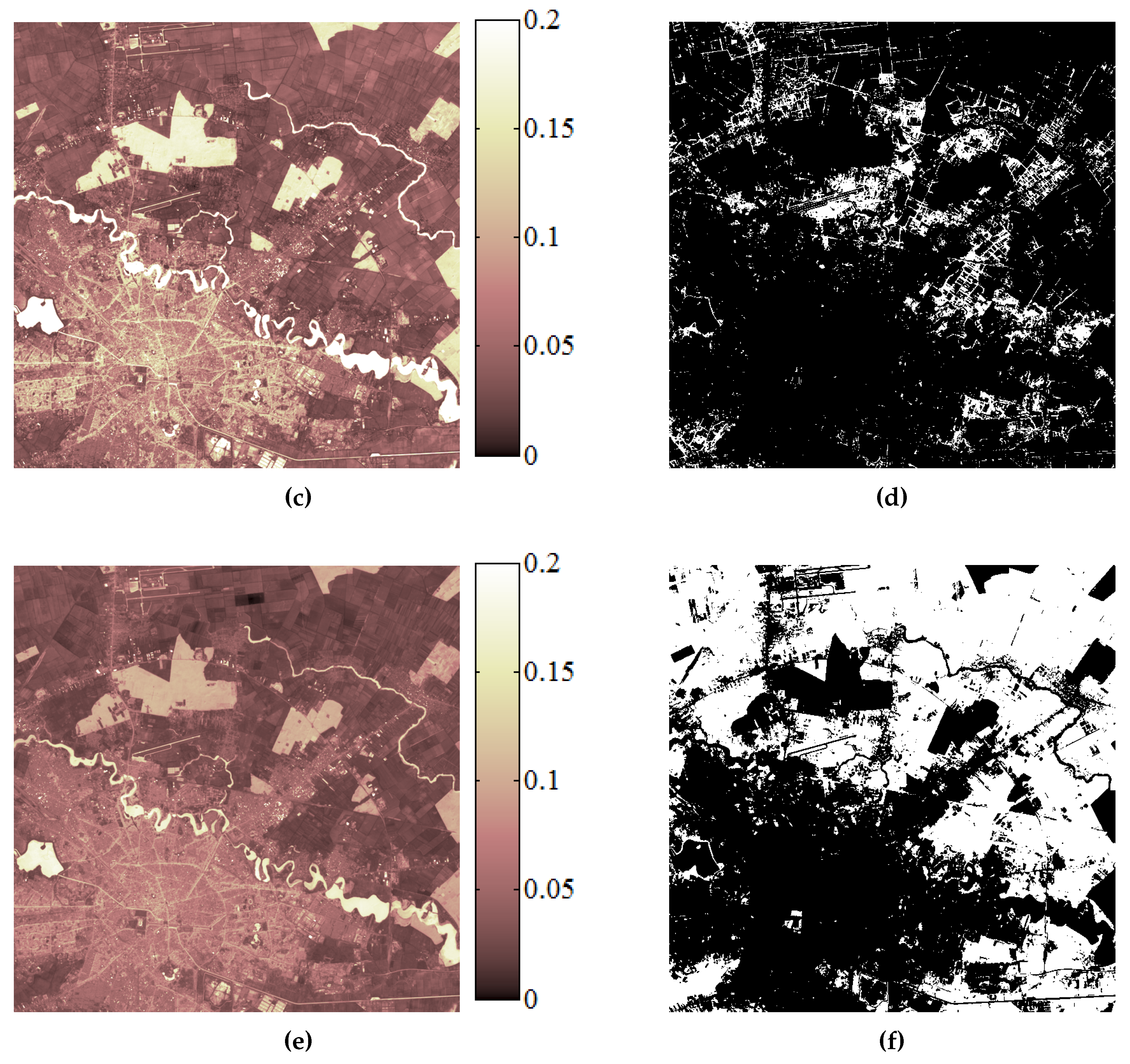
The second dataset is formed of 13 Landsat images of $1250\times 400$ pixels capturing the Dobrogea region, Romania, between 6 May 2000 and 9 September 2001. Some images from the dataset, together with the corresponding timespan, are shown in Figure 5. In May 2000, the heavy rain led to the swelling of Danube river which caused floods in this region (Figure 5a). A rapid assessment of the area affected by floods is necessary in this type of situation. Therefore, the application considered in this case was oriented towards the delimitation of areas affected by floods.

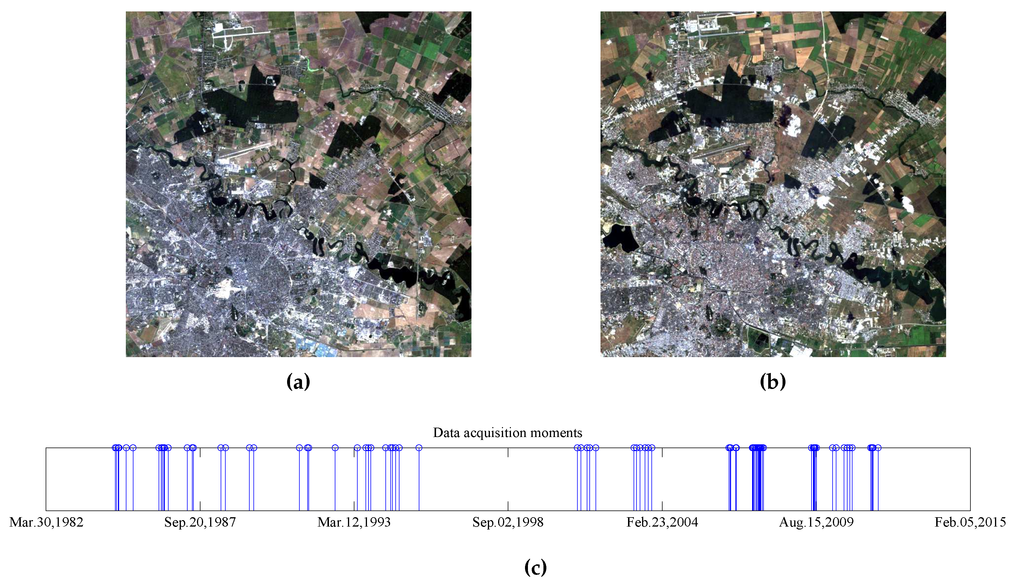
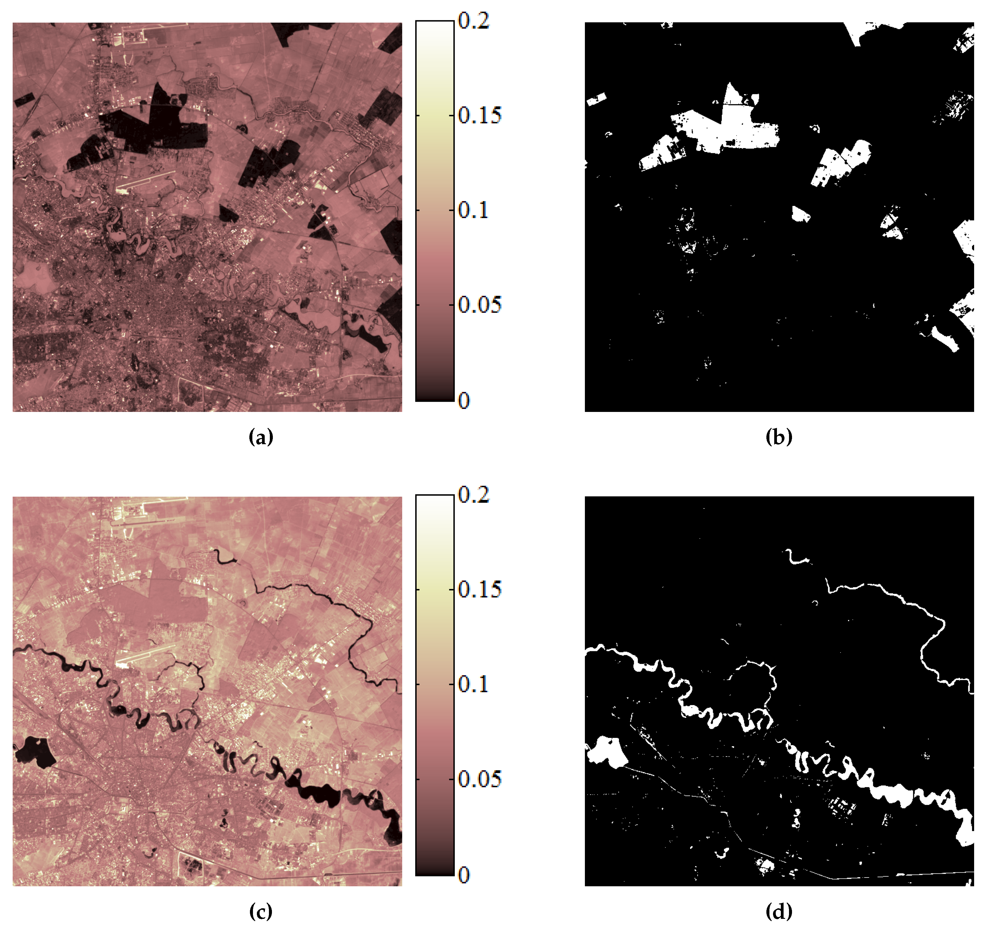
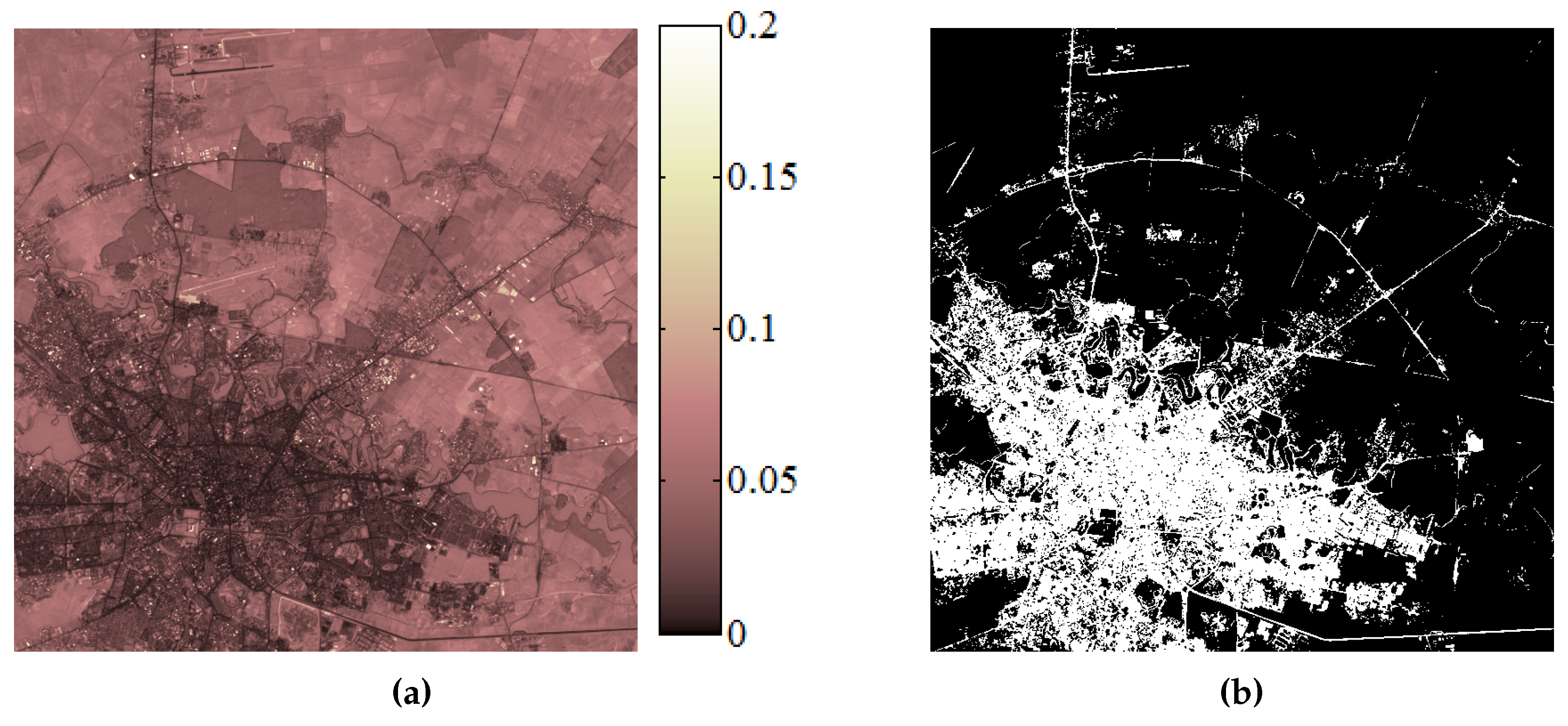
The third time series spans a longer period of time than the previous time series, almost 28 years between 14 September 1984 and 27 October 2011, and contains 88 multispectral images of $700\times 700$ pixels. The location is still Bucharest, Romania and surrounding regions, but the area captured by the SITS is smaller than in the previous case. 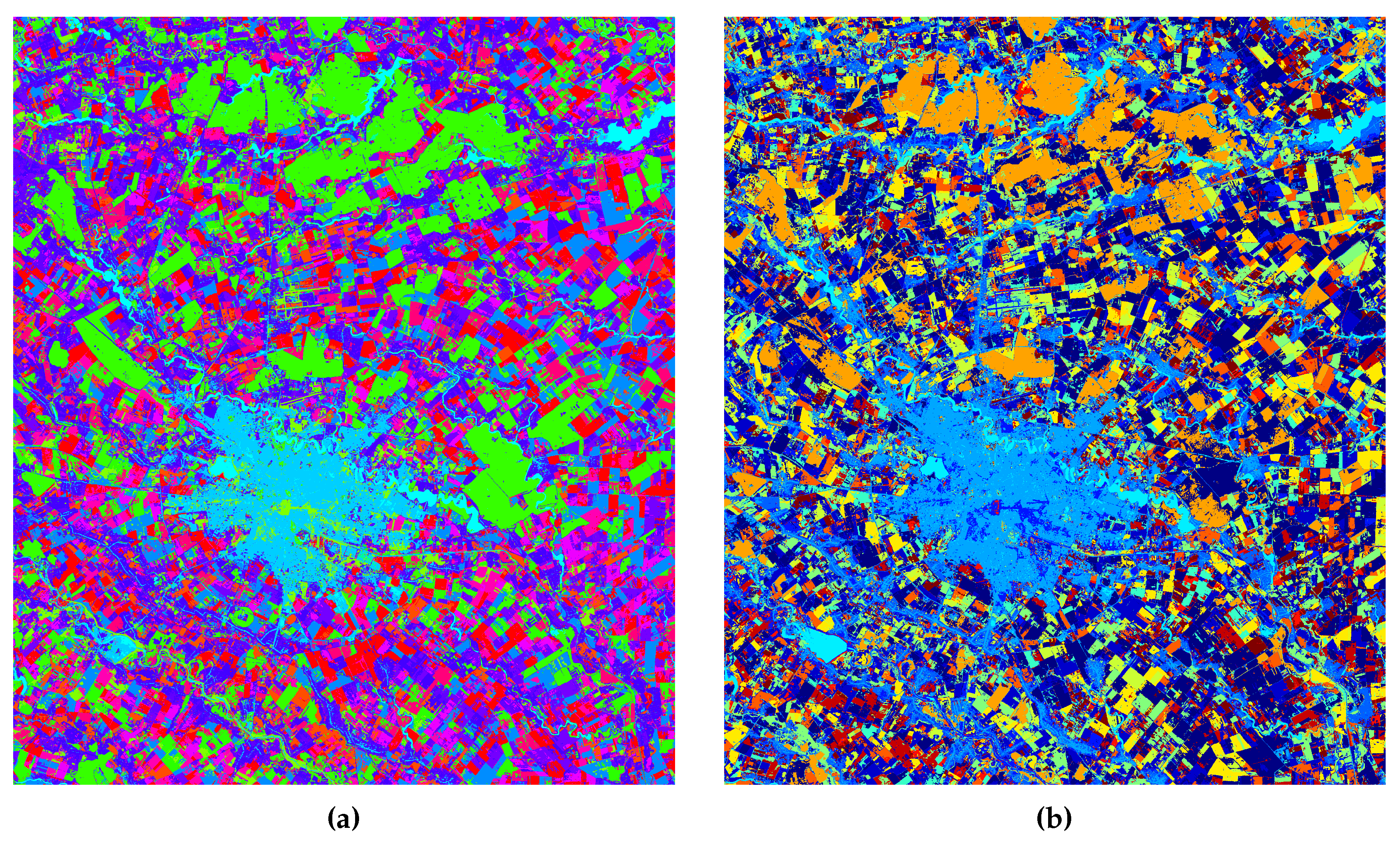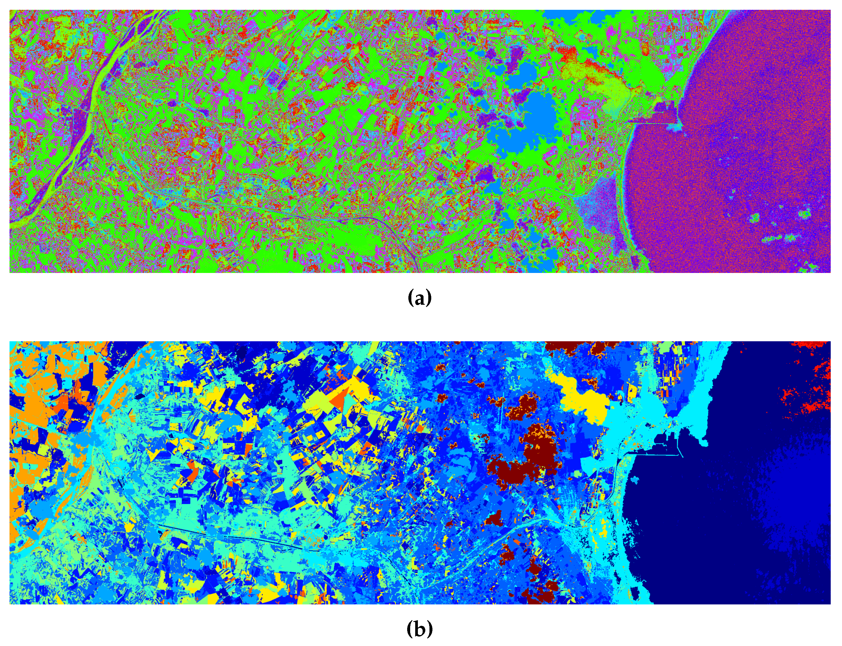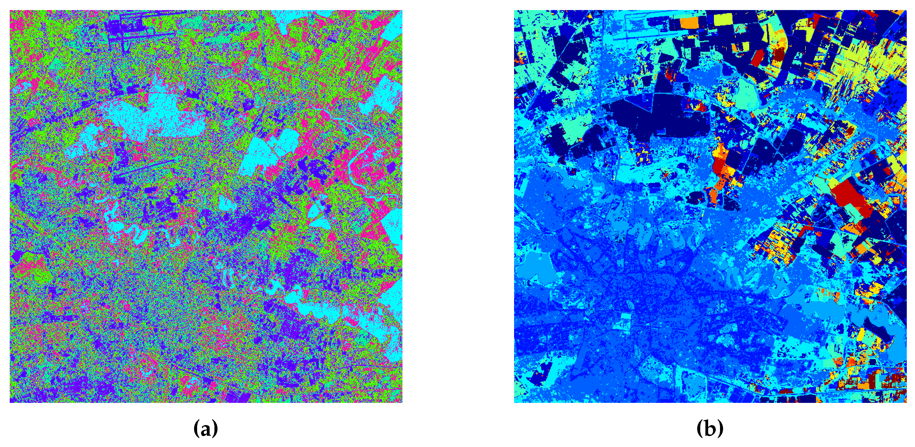The first and last images from the long-term SITS, along with the corresponding temporal distribution of the acquisitions, are shown in Figure 6. In general, long-term SITS acquisition is characterized by irregular temporal sampling with data captured under different meteorological (e.g., precipitation, clouds, season) and illumination conditions. These issues make the query-by-example retrieval in long-term SITS a challenging task to accomplish if other types of distance measure (e.g., Euclidean distance) are used to assess the degree of similarity between the temporal sequences. There are two main applications where the information extracted from long-term SITS shows its potential, namely land cover and land use mapping. These two applications impact the sustainable management of the natural resources, urban planning, and agriculture.

In all cases, the user was asked to select a single evolution in the area of interest and then the proposed algorithm was applied to identify other spatio-temporal evolutions with similar spectro-temporal signatures.

4. Discussion

4.1. Discovery of Similar Patterns in SITS

In the first setup, we aimed to discover two types of spatio-temporal evolution related to the formation of three accumulation lakes in the Bucharest region, namely Morii, Dridu and Mihailesti. If compared to the Morii and Dridu lakes, Lake Mihailesti has a distinct spatio-temporal evolution because this accumulation lake was emptied several times (in 1987 and in 1992) during its construction. The spectro-temporal differences between the two queries can also be observed from the spectro-temporal signatures shown in Figure 7. In this sense, the user performs two independent queries, each selected from the regions of interest. The analyzed period of time was between 1984 and 1993 and the dataset considered for retrieval was the short Landsat SITS composed of 10 images captured in the mentioned period (i.e., one image per year).

The results of the proposed query-by-example retrieval method are shown in Figure 8, whereas the ground truth is presented in Figure 9. The first row of Figure 8 represents all the DTW distances measured between the query and the rest of the spatio-temporal sequences, whereas the second row shows the output of the retrieval system (i.e., after applying the optimal threshold over the DTW distance image). For a numerical evaluation of the performances reached by the system, we measured the overall accuracy (OA), the missed alarm rate (MAR) and the false alarm rate (FAR), which are defined as

$$OA=\frac{TP+TN}{TP+TN+FP+FN}$$

(17)

$$\begin{array}{cc}\hfill MAR& =\frac{FN}{TP+FN}\hfill \end{array}$$

(18)

$$\begin{array}{cc}\hfill FAR& =\frac{FP}{TN+FP}\hfill \end{array}$$

(19)

where TP indicates the number of similar spatio-temporal evolutions that were correctly identified, TN indicates the number of non-similar spatio-temporal evolutions that were correctly identified, FP is the number of non-similar spatio-temporal evolutions that were determined as similar, and FN is the number of similar spatio-temporal evolutions that were determined to be non-similar to the given query.

The results, reported in

Table 2. Performance evaluation on short SITS.

Query	Overall Accuracy	Missed Alarm Rate	False Alarm Rate
Morii and Dridu	99.68%	26.84%	0.23%
Mihailesti	99.36%	30.36%	0.56%

, show that the system is able to accurately determine similar spatio-temporal patterns with respect to the given queries in term of overall accuracy and false alarm rate. The missed alarm rate can still be decreased if spatial constraints are imposed (i.e., similar sequences are more likely to be close to the query location, and, conversely, non-similar spatio-temporal evolutions are likely to be surrounded by other non-similar spatio-temporal evolutions). In this case, Markov Random Fields models can be employed [1], but they are difficult to use in SITS analysis due to their computational complexity. In addition, if the searched spatio-temporal evolutions are not compact (e.g., construction of new buildings), the solution may not achieve satisfactory results.

4.2. Damage Assessment

Undoubtedly, the retrieval of spatio-temporal patterns is extremely important when assessing the spatial and temporal extent of the transformations suffered by an area. In this experiment, we aimed to identify the area affected by the floods that occurred in 2000 in the Dobrogea region, Romania, and to identify their harmful effects over several months. As shown in Figure 5, the first image of the series was captured immediately after the Danube river swelled, whereas the rest of the images were acquired after the river began to retreat. The result of the query-by-example retrieval proposed method is shown Figure 10, along with the corresponding ground truth. The numerical evaluation of the performance achieved by the proposed algorithm is presented in

Table 3. Performance evaluation for delimitation of flooded areas in Dobrogea.

Query	Overall Accuracy	Missed Alarm Rate	False Alarm Rate
Flooded area	99.96%	2.36%	0.13%

and confirms the effectiveness of the method for delimiting specific areas, e.g., flooded areas in this particular case. An interesting aspect is the fact that DTW managed to bypass the problem of distorted data—the region of interest is partially occluded by clouds in the last image from the series, but the proposed algorithm was still able to correctly retrieve the spatio-temporal evolutions in the flooded area.

4.3. Land Cover and Land Use Mapping over Long Time Series

In the third setup, the application scenarios were related to the land cover and land use mapping using archives of SITS. Among the queries that we experimented with, we recalled the identification of extra-urban expansion, the demarcation of the urban area, the delimitation of forest areas, the discovery of agricultural areas, and the search for water bodies that remained unmodified over the years. However, due to the complexity of the SITS (i.e., containing 88 images captured over 27 years) and of the queries, the performance of the retrieval algorithm was assessed by visual inspection. The results shown in Figure 11 and Figure 12 with Figure 6 show that the retrieval system was able to discover the queried spatio-temporal patterns for land cover and land use mapping even when the data was irregularly sampled and images were captured under different meteorological and illumination conditions.

4.4. Comparison with Other State-of-the-Art SITS Analysis Methods

As mentioned in the Introduction, the DTW-based K-means algorithm [7] and the LDA-based method described in [12] are unsupervised clustering methods for SITS analysis. We show a series of results obtained by applying the above mentioned methods over the experimental datasets in Figure 13, Figure 14 and Figure 15. Following the recommendations in [12], the number of clusters considered was 15 and the dictionary was formed of 150 words. In the case of the DTW-based K-means method, we used the same number of clusters as for the LDA-based method.

As it can be observed in Figure 15, both algorithms produce land use and land cover maps, for which the assignation of a temporal meaning (i.e., action name or evolution name) to the clusters is a difficult task to accomplish. Moreover, the extraction of particular temporal evolutions is not easy, since, most often, the spectral and spatial characteristics inhibit the temporal properties of spatio-temporal evolutions. This happens mostly when the number of clusters, K, is small. However, in both cases, using a greater K leads to inconsistent results and to oversegmentation of the images caused by nonhomogeneus spatio-temporal evolutions, cloud cluttering, noise, different illumination conditions, or seasonal changes. Our proposed approach aims to overcome these drawbacks by retrieving specific spatio-temporal evolutions that, at the end of the retrieval process, will receive the semantic label of the query.

The LDA-based method performs an analysis of change map time series that is determined by applying different similarity measures. However, these similarity measures do not take the temporal extent of a transformation into account. This explains the insertion of the two different evolutions related to the building of accumulation lakes Morii & Dridu and Mihailesti into the same cluster as can be observed in Figure 13b. The DTW-based clustering divides the evolution of Mihailesti lake into two classes, one that corresponds to Morii & Dridu evolution and one that captures the evolution of Bucharest city. The SITS analysis method proposed in this paper is able to determine an optimal threshold that separates the two types of evolution related to the construction of the accumulation lakes to separate them from other types of evolutions. In contrast, the proposed query-by-example distinguishes between the two different spatio-temporal patterns, whose dissimilar evolutions can be observed in the corresponding spatio-temporal signatures shown in Figure 7.

In the second use-case scenario, the DTW-based K-means method includes the flooded region in a category containing a portion of the Black Sea captured on the right hand side of Figure 14a, whereas the LDA-based analysis does not distinguish this particular evolution from the rest of evolution patterns. Therefore, this event is not marked as a separate cluster of spatio-temporal evolutions on the resulting maps shown in Figure 14. On the contrary, the proposed query-by-example retrieval method also shows its potential in this use-case scenario by clearly delimiting the affected area and allowing estimation of the damaged surface.

4.5. Final Remarks

Finally, the running time for performing a query-by-example retrieval over the short Landsat SITS is 1 min 18 s/query, whereas over the long Landsat SITS, the running time is 10 min/query. The running times are considerably smaller than those required to perform unsupervised clustering of the spatio-temporal evolutions using the DTW-based K-means algorithm with $K=15$ classes, as presented in [7] (i.e., 38 min 17 s for the short SITS and approximately 16 h for the long SITS). A shorter running time was registered for the LDA-based method—almost 25 min for short SITS and approximately 2 h for the long SITS.

5. Conclusions

In this paper, we described an effective query-by-example retrieval system that can be used for the exploitation of Earth Observation SITS. The strategy is based on a two-step procedure. The first step consists of measuring the degree of similarity between a query provided by the user and other spatio-temporal evolutions in SITS. The second step consists of separating similar and non-similar patterns via an optimal thresholding technique applied over the DTW distance image obtained in the first step.

The experiments showed that, even if the SITS is irregularly sampled, affected by clouds or haze, or if the acquisitions are performed in different seasons and under different illumination conditions, the method is able to recognize specific patterns in SITS. In order to show the effectiveness and applicability of our proposed retrieval method, we considered several application scenarios. First, we considered the problem of retrieving similar spatio-temporal patterns from the SITS by analyzing a specific case, namely the construction of two accumulation lakes with different histories. In the second scenario, we exploited the proposed method to assess the damage that floods produce over a region. This is a typical scenario in emergency situations when a fast and effective evaluation of the affected areas is mandatory. In the last scenario, we considered long SITS and aimed to build land cover and land use maps that provide fundamental information for many applications, including change analysis, crop estimation, sustainable management of natural resources, and urbanization planning.

Being characterized by a low computational complexity, the proposed method for retrieving similar spatio-temporal evolutions based on a specific query represents a good candidate for the online analysis and annotation of SITS. Moreover, the method is designed to use the entire information provided by a multispectral remote sensing sensor, regardless of the number of spectral bands.

References

1. Bruzzone, L.; Prieto, D.F. Automatic analysis of the difference image for unsupervised change detection. IEEE Trans. Geosci. Remote Sens. 2000, 38, 1171–1182. [Google Scholar] [CrossRef]
2. Bovolo, F.; Bruzzone, L. A Theoretical Framework for Unsupervised Change Detection Based on Change Vector Analysis in the Polar Domain. IEEE Trans. Geosci. Remote Sens. 2007, 45, 218–236. [Google Scholar] [CrossRef] [Green Version]
3. Celik, T. Unsupervised Change Detection in Satellite Images Using Principal Component Analysis and k-Means Clustering. IEEE Geosci. Remote Sens. Lett. 2009, 6, 772–776. [Google Scholar] [CrossRef]
4. Radoi, A.; Datcu, M. Automatic Change Analysis in Satellite Images Using Binary Descriptors and Lloyd-Max Quantization. IEEE Geosci. Remote Sens. Lett. 2015, 12, 1223–1227. [Google Scholar] [CrossRef]
5. Rabiner, L.; Juang, B.H. Fundamentals of Speech Recognition; Prentice-Hall, Inc.: Upper Saddle River, NJ, USA, 1993. [Google Scholar]
6. Skutkova, H.; Vitek, M.; Babula, P.; Kizek, R.; Provaznik, I. Classification of genomic signals using dynamic time warping. BMC Bioinform. 2013, 14, S1. [Google Scholar] [CrossRef] [PubMed]
7. Petitjean, F.; Inglada, J.; Gancarski, P. Satellite Image Time Series Analysis Under Time Warping. IEEE Trans. Geosci. Remote Sens. 2012, 50, 3081–3095. [Google Scholar] [CrossRef]
8. Radoi, A.; Burileanu, C. Query-by-Example Retrieval in Satellite Image Time Series. In Proceedings of the 2018 41st International Conference on Telecommunications and Signal Processing (TSP), Athens, Greece, 4–6 July 2018; pp. 1–5. [Google Scholar] [CrossRef]
9. Maus, V.; Camara, G.; Cartaxo, R.; Sanchez, A.; Ramos, F.M.; de Queiroz, G.R. A Time-Weighted Dynamic Time Warping Method for Land-Use and Land-Cover Mapping. IEEE J. Sel. Top. Appl. Earth Obs. Remote Sens. 2016, 9, 3729–3739. [Google Scholar] [CrossRef]
10. Belgiu, M.; Csillik, O. Sentinel-2 cropland mapping using pixel-based and object-based time-weighted dynamic time warping analysis. Remote Sens. Environ. 2018, 204, 509–523. [Google Scholar] [CrossRef]
11. Tan, C.W.; Webb, G.; Petitjean, F. Indexing and classifying gigabytes of time series under time warping. In Proceedings of the 2017 SIAM International Conference on Data Mining, Houston, TX, USA, 27–29 April 2017. [Google Scholar]
12. Vaduva, C.; Costachioiu, T.; Patrascu, C.; Gavat, I.; Lazarescu, V.; Datcu, M. A Latent Analysis of Earth Surface Dynamic Evolution Using Change Map Time Series. IEEE Trans. Geosci. Remote Sens. 2013, 51, 2105–2118. [Google Scholar] [CrossRef] [Green Version]
13. Pelletier, C.; Valero, S.; Inglada, J.; Champion, N.; Dedieu, G. Assessing the robustness of Random Forests to map land cover with high resolution satellite image time series over large areas. Remote Sens. Environ. 2016, 187, 156–168. [Google Scholar] [CrossRef]
14. Julea, A.; Meger, N.; Bolon, P.; Rigotti, C.; Doin, M.P.; Lasserre, C.; Trouve, E.; Lazarescu, V.N. Unsupervised Spatiotemporal Mining of Satellite Image Time Series Using Grouped Frequent Sequential Patterns. IEEE Trans. Geosci. Remote Sens. 2011, 49, 1417–1430. [Google Scholar] [CrossRef]
15. Petitjean, F.; Gançarski, P.; Masseglia, F.; Forestier, G. Analysing Satellite Image Time Series by Means of Pattern Mining. In Intelligent Data Engineering and Automated Learning; Lecture Notes in Computer Science; Springer: Berlin/Heidelberg, Germany, 2010; Volume 6283, pp. 45–52. [Google Scholar]
16. Radoi, A.; Datcu, M. Spatio-temporal characterization in satellite image time series. In Proceedings of the 8th International Workshop on the Analysis of Multitemporal Remote Sensing Images, MultiTemp 2015, Annecy, France, 22–24 July 2015; pp. 1–4. [Google Scholar] [CrossRef]
17. Muller, M. Dynamic Time Warping. In Information Retrieval for Music and Motion; Springer: Berlin/Heidelberg, Germany, 2007; pp. 69–84. [Google Scholar] [CrossRef]
18. Redner, R.A.; Walker, H.F. Mixture Densities, Maximum Likelihood and the EM Algorithm. SIAM Rev. 1984, 26, 195–239. [Google Scholar] [CrossRef]
19. Bishop, C.M. Pattern Recognition and Machine Learning (Information Science and Statistics); Springer-Verlag New York, Inc.: Secaucus, NJ, USA, 2006. [Google Scholar]
Figure 1. Spectro-temporal signature in a Landsat satellite image time series (SITS).
Applsci 08 02435 g001
Figure 2. The flowchart of the proposed retrieval of similar patterns in SITS.
Applsci 08 02435 g002
Figure 3. Histogram over DTW similarity scores and a mixture of two Gaussian distributions fitted to these scores.
Applsci 08 02435 g003
Figure 4. Short Landsat SITS comprised of 10 images captured between 1984–1993. Only four representative images (i.e., containing specific changes) of the series are shown: (a) 1984, (b) 1987, (c) 1988, (d) 1992. The distribution of the acquisition moments is shown in (e).
Applsci 08 02435 g004
Figure 5. Dobrogea Landsat SITS comprised of 13 images captured between 6 May 2000 and 14 September 2001, in the Dobrogea region. Four images of the series are shown, namely: (a) 6 May 2000, (b) 22 May 2000, (c) 9 July 2000, and (d) 29 October 2000. The distribution of the acquisition moments is shown in (e).
Applsci 08 02435 g005
Figure 6. Long Landsat SITS comprised of 88 images captured in 1984–2011. Only the first and the last images of the series are shown, namely (a) 1984 and (b) 2011. The distribution of the acquisition moments is shown in (c).
Applsci 08 02435 g006
Figure 7. Spectro-temporal signatures during the construction of the accumulation lakes. The two spectro-temporal signatures are characterized by different temporal evolutions in the period that corresponds to their construction, namely 1984–1993.
Applsci 08 02435 g007
Figure 8. Pattern discovery in short Landsat SITS. (a) DTW distance image for a query marked inside the Morii & Dridu accumulation lakes. (b) DTW distance image for a query marked inside Mihailesti accumulation lake. (c) Pattern discovery using the proposed method for Morii & Dridu accumulation lakes. (d) Pattern discovery using the proposed method for Mihailesti accumulation lake. In the case of DTW distance images presented in (a,b), dark color represents similar evolutions and bright color represents non-similar evolutions, whereas in (c,d), white pixels correspond to spatio-temporal patterns that are similar to the query, which was selected from the region of interest.
Applsci 08 02435 g008
Figure 9. Ground truth for short Landsat SITS. White pixels delimit (a) Morii & Dridu accumulation lakes and (b) Mihailesti accumulation lake.
Applsci 08 02435 g009
Figure 10. Delimitation of areas affected by floods in Dobrogea. (a) DTW distance image for a query in the flooded area. (b) Delimitation of the affected area using the proposed algorithm. (c) Ground truth marking the flooded areas. In the case of DTW distance image presented in (a), dark color represents similar evolutions and bright color represents non-similar evolutions, whereas in (b) white pixels correspond to spatio-temporal patterns that are similar to the query, which was selected from the region of interest.
Applsci 08 02435 g010
Figure 11. Land cover mapping in long Landsat SITS. (a) DTW distance image for a query made inside the forestry area. (b) Forestry area delimitation using the proposed query-by-example retrieval method. (c) DTW distance image for a query made in an area covered by water. (d) Water delimitation using the proposed query-by-example retrieval method. In the case of DTW distance images presented in (a,c), dark color represents similar evolutions and bright color represents non-similar evolutions, whereas in (b,d), white pixels correspond to spatio-temporal patterns that are similar to the query, which was selected from the region of interest.
Applsci 08 02435 g011
Figure 12. Land use mapping in long Landsat SITS. (a) DTW distance image for a query made in the urban area. (b) Urban area delimitation using the proposed query-by-example retrieval method. (c) DTW distance image for a query made in the extra-urban area. (d) Extra-urban area delimitation using the proposed query-by-example retrieval method. (d) DTW distance image for a query made inside the agricultural area. (e) Agricultural area delimitation using the proposed query-by-example retrieval method. In the case of DTW distance images presented in (a,c,e), dark color represents similar evolutions and bright color represents non-similar evolutions, whereas in (b,d,f), white pixels correspond to spatio-temporal patterns that are similar to the query, which was selected from the region of interest.
Applsci 08 02435 g012aApplsci 08 02435 g012b
Figure 13. Analysis of short Landsat SITS: (a) DTW-based K-means clustering [7], (b) LDA-based clustering [12].
Applsci 08 02435 g013
Figure 14. Analysis of Dobrogea SITS: (a) DTW-based K-means clustering [7], (b) Latent Dirichlet Allocation (LDA)-based clustering [12].
Applsci 08 02435 g014
Figure 15. Analysis of long Landsat SITS: (a) DTW-based K-means clustering [7], (b) LDA-based clustering [12].
Applsci 08 02435 g015