Settlement Prediction and Differential Settlement Criterion for Heightening and Thickening Levee

Abstract

Owing to the pavement cracking of heightening and thickening levees (HTL) caused by differential settlement, it is necessary to study the settlement prediction and differential settlement criterion for HTLs. In this study, an HTL was taken as the study object. First, leveling observation and layered settlement observation were adopted, and a generalized settlement prediction model (GSPM) that can describe both S-shaped and hyperbolic settlement–time curves was proposed. The physical meanings of GSPM parameters were analyzed. Moreover, the effectiveness of the GSPM was verified using field monitoring data. Second, finite element analysis based on a viscoelastic constitutive model was used to reveal the quantitative relationship between the differential settlement and horizontal stress of the pavement. On this basis, the differential settlement criterion was obtained. The results showed that the GSPM can unify the logistic model and hyperbolic model by introducing two morphological change parameters. In addition, the GSPM can be more widely used, more accurate, and more stable than the traditional logistic model and hyperbolic model. When an asphalt concrete pavement (whose ultimate tensile stress is 0.12 MPa) is used, the corresponding differential settlement criterion is approximately 4.3 cm. The research results can provide a reference for reasonable differential settlement control for HTLs in order to prevent pavement cracking.

1. Introduction

Most levees have been constructed from soil, and many years of service may have caused various types of damage to them. Therefore, it is necessary to reinforce the old levees. Heightening and thickening of levees is a common method to reinforce old levees, but differential settlement of the heightening and thickening levee (HTL) may be caused by the uneven foundation and the compressibility difference between the backfill and the old levee. As a result, excessive differential settlement may cause cracks on the levee pavement and weaken its flood control capacity further. The pavement cracking of practical engineering is shown in Figure 1. The cracking shortens the life of the pavement. In addition, rainwater extending along cracks reduces the stability of the HTL further. In particular, the transverse cracks caused by differential settlement may bring about a levee breach. The consequences of a levee breach may be catastrophic. Therefore, it is necessary to study the differential settlement of the HTL.

At present, settlement prediction [1,2] has been studied by many engineers in structures such as tunnels [3,4], high-speed railways [5,6], bridges [7,8], and levees [9,10]. In general, settlement prediction methods can be divided into two categories: Numerical calculations and deducing methods based on field data. Numerical methods [11] include the finite element method [12] and difference method, but these methods are limited by the constitutive model, the determination of material parameters, and the boundary conditions. However, deducing methods based on field monitoring data can overcome these issues. For deducing methods, there are mainly seven types: 1. Hyperbolic model [13,14]; 2. Exponential curve model [15,16,17]; 3. Three point method [18,19,20]; 4. Asaoka method [21,22]; 5. Logistic curve method [23]; 6. Grey theory method [24,25]; and 7. Neural network [26,27,28].

In fact, the settlement–time curve of the HTL shows variation. The settlement–time curve variation of the HTL may be due to factors such as seepage, erosion, groundwater changes, freeze–thaw deformation, and the initial time-point of monitoring. In addition, settlement–time curve variation has also been shown in a previous study [29] involving an expressway. Hence, the traditional logistic model and hyperbolic model are inadequate to describe the settlement–time curve variation, which may result in settlement prediction errors, such as final settlement error and settlement stability time error. Therefore, finding a settlement prediction model with strong adaptability and strong stability is still a challenge.

However, the differential settlement of the HTL is unavoidable in practical engineering. It must be pointed out that differential settlement that does not cause pavement cracking is acceptable. Regrettably, the control criterion of the differential settlement for the HTL is still unclear at present, which leads to uncertainty in settlement control. Therefore, it is necessary to identify the differential settlement control criterion for the HTL from the point of view of the pavement cracking mechanism.

This paper can be divided into two parts. First, a generalized settlement prediction model (GSPM) describing an S-shaped and hyperbolic settlement–time curve is proposed. In the first part, the physical meaning of the model parameters is analyzed, and the effectiveness of the GSPM is validated using field monitoring data. For the second part, the differential settlement control criterion is presented based on the finite element method. The two parts, which are closely related, can provide a reference to achieve reasonable differential settlement control of the HTL in order to prevent pavement cracking.

2. Methodology

There are some differences between a new levee and an HTL. For an HTL, the compressibility of the old levee and old foundation is very low. The deformation mainly arises owing to the backfill and new foundation. Hence, the settlement prediction method and settlement control criterion are different from those of the new levee.

This section focuses on four aspects. They are a generalized model, a generalized settlement prediction model, settlement monitoring, and a finite element method. These four aspects have a certain logical relationship because settlement prediction needs a settlement criterion to clarify the position that needs to be controlled. Hence, settlement prediction and the settlement control criterion are interdependent.

2.1. Generalized Model

Figure 2 shows the generalized model of the HTL. In fact, there are three ways to increase the height and thickness. However, heightening and thickening along the downstream slope is more common. Hence, the heightening and thickening along the downstream slope is taken as the generalized model.

For the HTL, pavement cracks mainly occur on the downstream slope, as shown in Figure 1a. In fact, there are different kinds of pavement failure. Hence, there are different mechanisms accounting for pavement failure, such as leakage, flood scour, and differential settlement (see Figure 1a,b). In essence, all the pavement failure mentioned above can result from large settlements. In this paper, pavement cracking is the main research question. The main characteristic of this kind of crack is located at the junction of the backfill and the old levee. The cracking is due to the differential settlement.

The HTL is mainly composed of the old levee, backfill, and pavement. The differential settlement of the HTL may cause early cracking of the pavement, which shortens the life of the pavement and reduces the stability of the HTL. The main reasons for differential settlement are as follow: 1. The compressibility between the old levee and backfill soil is different; 2. The foundation is uneven.

In general, the compressibility of the backfill is higher than that of the old levee because the compactness of the old levee is high under long-term loading. In turn, the backfill is not compacted and has rheological characteristics. Moreover, the consolidation of the backfill is very small, according to the author’s settlement monitoring. The settlement of the backfill mainly comes from rheology. However, the consolidation of the new foundation still exists and is not universal. Hence, this study focuses on the rheology of the backfill.

In this paper, a generalized settlement prediction method is described so that the pavement laying time can be determined. On this basis, the relationship between the horizontal stress of the pavement and differential settlement will be revealed based on finite element analysis.

2.2. Generalized Settlement Prediction Model (GSPM)

The settlement prediction method based on numerical calculation is limited by the constitutive model of soil, boundary conditions, determination of parameters, and other factors. Therefore, a generalized settlement prediction model based on settlement monitoring was adopted in this study to predict settlement.

A GSPM was proposed because of the variability of the settlement–time curve. The variability reduces the accuracy of settlement prediction. The reasons for the variability of settlement–time curves are as follow: 1. It is related to the starting point of the monitoring time. If the settlement during the construction period is considered, the settlement–time curve tends to an S-type [30]; if only postconstruction settlement is considered, the settlement–time curve tends to a hyperbolic type. 2. In fact, postconstruction settlement can be S-type as well, which may be related to seepage during the flood season. Seepage deformation, such as piping and soil flow, may occur during flood season. Therefore, the postconstruction settlement from flood season to nonflood season may still be S-shaped. 3. Postconstruction settlement is affected by ambient temperature. The freezing and thawing cycle of soil can cause the settlement–time curve to be S-type as well. In short, it is necessary to propose a generalized settlement prediction model to adapt to the variability of the settlement–time curve.

2.2.1. Physical Meaning of Parameters

Accurate geotechnical settlement prediction is very difficult, or even impossible, because there are many influencing factors with a certain degree of randomness and variability. In a sense, the actual settlement–time curve is not always a single form [31], such as hyperbolic or S-type. The traditional settlement prediction model cannot predict both hyperbolic and S-type settlement simultaneously. Hence, a GSPM that follows Equation (1) is suggested. The idea of this model comes from the logistic model and the hyperbolic model. The denominator of this model is the imitation of the logistic model, and the numerator part of GSPM is the imitation of the hyperbolic model. The significance of Equation (1) is that it does not need to change the model when the concrete fitting operation is carried out because this model has already unified the S-type model and the hyperbolic model.

$$y\left(t\right)=\frac{a(1-e^{\frac{-t}{b}})}{d{e}^{\frac{-t}{c}}+1}$$

(1)

Here, a, b, c, and d are parameters; t is time; y(t) is settlement.

The descriptive ability of the model is given in Figure 3. From Figure 3a, parameter a means final settlement. From Figure 3b, parameter b means the settlement stabilization time. The smaller parameter b is, the shorter the settlement stabilization time will be. Parameters a and b have a conventional meaning. However, parameter c and d are different from the traditional logistic model and hyperbolic model based on Figure 3c,d. Hence, parameters c and d can be called morphological change parameters.

When d = 0, the GSPM can be written as $y\left(t\right)=\mathrm{a}(1-e^{\frac{-t}{b}})$. Hence, parameter c has no effect when d = 0. This means that the GSPM can describe a hyperbolic settlement–time curve when d = 0. When d ≠ 0, GSPM can describe an S-shaped settlement–time curve. Hence, physically, parameter d indicates a morphological switch. Moreover, parameter c also describes settlement stabilization time when d ≠ 0.

2.2.2. Further Explanation of Physical Meaning of Parameters

The comparison of different prediction models has been listed in

Table 1. Comparison of different prediction models.

Models	GSPM	Logistic Model [29,32,33]	Hyperbolic Model [13,14,34,35]
Expression	$y\left(t\right)=-\frac{a(1-e^{-\frac{t}{b}})}{d{e}^{-\frac{t}{c}}+1}$	$y\left(t\right)=\frac{k}{a_2{e}^{-b_{1}t}+1}$	$y\left(t\right)=\frac{t}{a_1+\mathrm{t}}{S}_{\infty }$
Descriptive ability	Both S-shaped and hyperbolic curve	Only S-shaped curve	Only hyperbolic curve
Number of parameters	4	3	2

. The GSPM can describe both S-shaped and hyperbolic curves because it has four parameters. In fact, the present settlement data are sufficient to fit four parameters, and the specific fitting method is carried out using Mathematica.

In this section, the physical meaning of parameters is explained via comparisons with different models. The following equation symbols are listed in Table 1. The explanation is as follows:

First, the equivalence between the GSPM and logistic model will be discussed. For Equation (1), when $b\to \infty$ then $a(1-{\mathrm{e}}^{-\frac{t}{b}})\to a$.

When $-a=k\mathrm{and}d=a_2\mathrm{and}\frac{1}{c}=b_1$, the GSPM and logistic model are the same, i.e., the logistic model is a special case of the GSPM. Under these circumstances, the physical meaning of parameters from the GSPM can be explained from the perspective of the logistic model. Parameters a and k have the same physical meaning. Parameters d and $a_2$ have the same physical meaning. Parameters c and $b_1$ have the same physical meaning.

Second, the equivalence between the GSPM and hyperbolic model will be discussed.

The hyperbolic model can be written as follows:

$$y\left(t\right)=\frac{t}{a_1+\mathrm{t}}{S}_{\infty }.$$

(2)

However, when $d=0$, the GSPM can be written as:

$$y\left(t\right)=-a(1-e^{-\frac{t}{b}}).$$

(3)

If the GSPM and the hyperbolic model are the same, then

$$\{\begin{array}{c}-a=S_{\infty }\\ \frac{t}{a_1+t}=1-e^{-\frac{t}{b}}\end{array}.$$

(4)

Mathematica 11.3 will be used to solve Equation (4) and the result is shown as Equation (5):

$$b=-\frac{t}{l{n}^{\frac{a_1}{a_1+t}}}$$

(5)

Equation (5) can demonstrate that the hyperbolic model is a special case of the GSPM. Hence, the physical meaning of parameters from the GSPM can be explained from the perspective of the hyperbolic model. Parameters b and $a_1$ have the same physical meaning in such a situation.

Hence, equivalence between the GSPM and previous models (logistic model and hyperbolic model) has been explained. Moreover, the physical meaning of the GSPM parameters can also be explained based on the hyperbolic model and logistic model.

2.2.3. The Significance of GSPM

The significance of GSPM is to unify the logistic model and hyperbolic model by introducing two morphological change parameters. The reasons are as follows:

• Two morphological change parameters (c and d) were introduced into the GSPM (see Figure 3c,d).
• When d = 0, the GSPM can be written as $y\left(t\right)=a(1-e^{\frac{-t}{b}})$. Moreover, Equation (5) can demonstrate that the hyperbolic model is a special case of the GSPM. This means that the GSPM can describe a hyperbolic settlement–time curve when d = 0.
• When d ≠ 0, $-a=k\mathrm{and}d=a_2\mathrm{and}\frac{1}{c}=b_1$, the GSPM and logistic model are the same, i.e., the logistic model is a special case of the GSPM. Hence, GSPM can describe an S-shaped settlement–time curve.

2.3. Settlement Monitoring

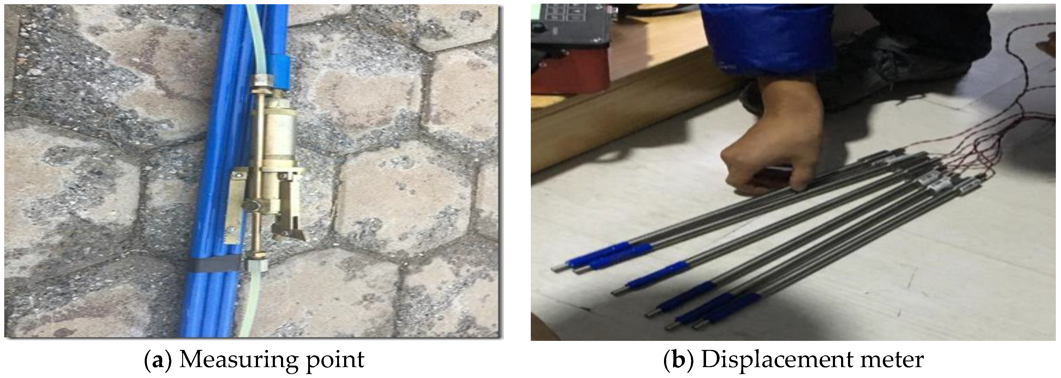
This monitoring mainly involves ground leveling observation and internal settlement observation. The leveling is used for leveling observation, and the multipoint displacement meter is used for internal settlement observation. Figure 4 shows the monitoring instruments. The measuring point layout is shown in Figure 8. The field monitoring is from 20 October 2016 to 1 July 2017. The monitoring cycle is approximately 15 days. The monitoring began when construction was completed. Hence, the settlement from monitoring is the postconstruction settlement.

To obtain the internal settlement law, a multipoint displacement meter was used to monitor the internal settlement. It should be noted that the internal settlement monitoring is not independent of the leveling observation. The leveling observation represents the absolute settlement value, and the multipoint displacement meter is a relative settlement value relative to point A and point B, shown as Figure 8. The relationship between them is as follows (Equations (6) and (7)). The internal absolute settlement of the HTL is equal to the surface level settlement plus the internal relative settlement monitoring value.

$$S_i^B=S_B+S_i \left(i=1,2,3\right)$$

(6)

$$S_i^A=S_A+S_i \left(i=4,5,6\right)$$

(7)

Here, $S_A\mathrm{and}{S}_B$ is the absolute settlement of point A and point B, shown in Figure 8. $S_i\left(i=1,2\dots 6\right)$ is the relative settlement, relative to the point A and point B shown in Figure 8. $S_A\mathrm{and}{S}_B$ are from the leveling observation. $S_i\left(i=1,2\dots 6\right)$ is from the multipoint displacement meter. $S_i^B$ and $S_i^A$ are absolute settlement values.

2.4. Finite Element Analysis

Because of the limitation of the geometric model of the old levee, the traditional stratified summation method is not suitable. In addition, it is also hard to consider the viscoelastic constitutive model of backfill in a traditional stratified summation method. Therefore, the finite element analysis is used in this study to analyze the settlement.

2.4.1. Viscoelastic Constitutive Model

In fact, there is a difference between the HTL and the new levee. On the one hand, owing to long time compaction and consolidation, the compressibility of the old levee and old foundation is very low because the consolidation effect of the old levee and the old levee foundation have basically been completed. For the case study, the deformation of the HTL mainly comes from the rheology of backfill.

Hence, the viscoelastic constitutive model is adopted in this study. The model can describe the viscoelastic behavior of shear and volume change. In addition, the differential settlement increases with time and finally tends to be stable. However, the viscoelastic constitutive model can describe the shear and time effect. Hence, the viscoelastic constitutive model is suitable to describe the settlement rules of the HTL.

However, it is very difficult to determine the parameters of the existing complex viscoelastic model, and the settlement of the HTL gradually decreases with time and finally tends to be stable. Therefore, in this study, it is more appropriate to choose the merchant model to describe settlement.

The one-dimensional merchant model is shown in Figure 5. It is composed of a Hook body and Kelvin body, as shown in Figure 5. Its model parameters include instantaneous elastic modulus $E_H$, viscoelastic modulus $E_K$, and viscous coefficient ${\eta }_K$.

2.4.2. Determination of Calculation Parameters

ABAQUS is one of the most advanced finite element software packages in the world at present, but it does not directly provide the merchant model based on one-dimensional tension–compression viscoelastic parameters. ABAQUS adopts an integral constitutive equation of shear relaxation modulus and bulk relaxation modulus based on Prony series. To utilize the powerful numerical calculation ability of ABAQUS, it is necessary to establish the relationship between the viscoelastic parameters of a one-dimensional merchant model and the integral constitutive model parameters adopted by ABAQUS.

A previous study [36] has provided the determination method for parameters. The method is as follows:

$$G\left(0\right)=G_H$$

(8)

$${\tau }_1^G=\frac{{\eta }_K^G}{G_H+G_K}$$

(9)

$$g_1=\frac{G_H}{G_H+G_K}$$

(10)

$$G_H=\frac{E_H}{2\left(1+{\upsilon }_H\right)}$$

(11)

$$G_K=\frac{E_K}{2\left(1+{\upsilon }_K\right)}$$

(12)

$${\eta }_K^G=\frac{{\eta }_K}{2\left(1+{\upsilon }_K\right)}$$

(13)

Here, $G\left(0\right)$ is the instantaneous shear modulus. $G_H$, $G_K$, and ${\eta }_K^G$ are parameters of the shear viscoelastic parameters of the Merchant model. ${\upsilon }_H$ and ${\upsilon }_K$ are the Poisson’s ratio corresponding to the Hook body and the Kelvin body of the merchant model. Usually, ${\upsilon }_H={\upsilon }_K=\upsilon$.

The material parameters used for calculation are listed in

Table 2. Material parameters for calculation.

Structure Type	Weight (kN/m3)	$\mathbf{Young}’\mathbf{s}\mathbf{Modulus}{\mathit{E}}_{\mathit{H}}\left(\mathbf{MPa}\right)$	$\mathbf{Young}’\mathbf{s}\mathbf{Modulus}{\mathit{E}}_{\mathit{K}}\left(\mathbf{MPa}\right)$	Long-Term Elastic Modulus (MPa)	Poisson Ratio	$\mathbf{Viscosity}\mathbf{Coefficient}{\mathit{\eta }}_{\mathit{K}}(\mathbf{MPa}·\mathbf{d})$
Old levee	14.1			30	0.35
Foundation	14.7			30	0.35
Backfill	14.1	60	60		0.35	9380
Pavement	22			1200	0.25

. The determination of material parameters is mainly based on the following considerations: 1. The long-term deformation modulus of a levee is 30 MPa, based on Table 4; 2. It is assumed that both instantaneous deformation and viscoelastic deformation are 50% of total deformation [36]. Based on this assumption, $E_H$ and $E_K$ can be determined. 3. It is assumed that viscoelastic deformation can reach 90% in 1 year [36]. Based on this assumption, ${\eta }_K$ can be determined.

2.4.3. Mesh of HTL

The 2D mesh is shown in Figure 6. In this study, CPS4R is applied for the calculation. The CPS4R is a 4-node bilinear plane stress quadrilateral, reduced integration, hourglass control. In the calculation, the visco step is adopted.

The pavement width of this model is 10 m. The slope is 1:3. The height of the old levee is 3.5 m. The heightening is 1 m. The thickening is 4 m. The depth of the foundation is 10 m.

The criteria to mesh are as follow:

• The technology of free mesh generation is adopted, which can guarantee the mesh analysis errors and warnings are 0%;
• The advancing front algorithm (use mapped meshing where appropriate) is adopted, which can guarantee the mesh analysis errors and warnings are 0%;
• The element shape is mainly quad-dominated and contains a small number of triangular elements. This can also guarantee the mesh analysis errors and warnings are 0%;
• The approximate global size is 0.25 m; for curvature control, the maximum deviation factor is 0.1; for minimum size control, the fraction of global size is 0.1.

In fact, the accuracy of finite element calculation depends on the quality and quantity of mesh. The four aspects above can guarantee mesh quality. In order to guarantee the accuracy of calculation, it is necessary to perform a mesh sensitivity analysis. The mesh sizes are 0.25 m, 0.2 m, 0.15 m, and 0.1 m respectively in the analysis. The results are shown in Figure 7. The three results are almost the same, which demonstrates that mesh sizes (0.25 m) in this paper are reasonable.

2.4.4. Boundary Conditions

Boundary conditions are influenced by the environment, adding to the complexity. Considering all the boundary effects will reduce calculation efficiency and is also unnecessary. For the monitoring section, there are several facts: 1. Antiseepage treatment has been performed on the upstream slope. Hence, the seepage deformation of the HTL is small. 2. The water level of the river is under the foundation during the nonflood season because the monitoring section belongs to the detention basin. 3. The consolidation of the old levee and old foundation is small. 4. The major deformation comes from the rheology of the backfill. 4. Because the HTL section studied is not located at the meizoseismal area, the dynamic load is not taken into account in the calculation.

The main load is the vehicle load at the top of the HTL. Therefore, the load boundary in this study only considers the vehicle load at the top of the HTL.

Specifically, uniform loads of 10 kPa, 15 kPa, and 20 kPa are applied to simulate the vehicle load on the top of the pavement.

For the displacement boundary condition, the bottom of the HTL is a fixed constraint, and the head and end of the HTL is the normal constraint.

3. Case Study

3.1. Case Introduction

The case study considers a location at the Songhua River in Harbin, China. The HTL is an important protection infrastructure for the city of Harbin. Harbin is located in the north of China, which is characterized by seasonally freezing–thawing areas. Moreover, Section II of the monitoring is located in BaCha of the Heilongjiang Province.

The case that belongs to the detention basin is along Songhua River. The average height of the levee is 3 m–5 m, and the slope is 1:2–1:5. The existing flood control standards are about once in 15 years. The HTL length is not constant along the length. The pavement width of the first-grade HTL is 10 m. The pavement width of the second-grade HTL is 8 m. The pavement width of others is 6 m. For most of the HTLs, the slope is 1:3 and the pavement width is 8m.

In this study, heightening and thickening along the downstream slope is chosen for investigation. In the following text, this case will be taken as a case study. It will proceed from the following 4 aspects.

3.1.1. Selection of Monitoring Section

According to the design data, the main levee in the Heilongjiang mainstream is the Earth levee, which accounted for more than 70%. The sand levee accounted for about 18%. The remaining was a soil–sand mixed levee. The characteristics of each type of levee are outlined in

Table 3. Levee characteristics.

Type of Levee	Characteristics
Earth levee	Good compactness, permeability coefficient 10−5 cm/s, good impermeability.
Sand levee	With sand and gravel, the allowable bearing capacity is greater than 100 kPa, and the permeability stability is good.
Mixed levee	Upper layer is silty soil and clay. The down layer is poorly graded sand, gravel with poor permeability stability.

.

Hence, the earth levee is representative, which is one of reasons for determination of monitoring section. Moreover, the other reasons were as follow:

• The backfill here is large. Thickening is approximately 1 m. Heightening is approximately 0.5 m.
• The monitoring section is near a meandering river and the flow characteristics are more complex during flood season.
• The monitoring site is convenient.
• The monitoring site is an important levee for flood control in Harbin.

3.1.2. Material Parameters

To obtain soil parameters, we performed a site soil test and laboratory test. The soil parameters awee obtained at the Hohai University laboratory. The soil parameters included density, Young’s modulus, and other factors. The main apparatuses were balance, cutting ring, high pressure consolidation apparatus, and triaxial apparatus. The three main test procedures were as follow:

(1)

For the determination of dry weight, the main test apparatuses included cutting rings, balances, and ovens. The specific test steps were as follow:

Step 1: Cutting rings and balances were used to get the density of samples;

Step 2: Ovens were used to get the water content of samples;

Step 3: Calculate the dry density of soil samples using the Equation (14):

$${\gamma }_d=\frac{\rho g}{1+\omega }.$$

(14)

where $\omega$ is water content; $\rho$ is density of samples; $g$ is acceleration of gravity;

(2)

For the determination of the shear strength index, such as the cohesive and internal friction angle, the main test apparatus was a triaxial apparatus. The triaxial test was consolidated and undrained. The reasons for the selection are follow: 1. The soil at the scene belongs to normally consolidated soil; 2. After completion, there are a large number of vehicles loads on the top of the HLT. In the consolidated–undrained test, the specimen has been consolidated to a certain water content under the consolidation pressure and then sheared with constant water content.

(3)

For the determination of Young’s modulus, the main test apparatus was a high pressure consolidation apparatus. The specific steps are as follows:

Step 1: Assembly and commissioning of samples and apparatus;

Step 2: Initial pressure (1 kPa) is applied to ensure good contact and record initial data;

Step 3: Apply pressure (12.5 kPa, 25 kPa, 50 kPa, 100 kPa, 200 kPa, 400 kPa) at all levels and record data;

Step 4: Processing test data. The main formula is in Equations (15)–(19)

$$e_0=\frac{G_s{\rho }_w}{{\rho }_d}-1$$

(15)

$$e_i=e_0-\frac{1+e_0}{h_0}\Delta h_i$$

(16)

$$a_{\mathrm{v}}=\frac{e_i-e_{i+1}}{P_{i+1}-P_i}$$

(17)

$$E_S=\frac{1+e_0}{a_v}$$

(18)

$$E_0=\frac{\left(1+\mu \right)\left(1-2\mu \right)}{1-\mathsf{\mu }}{E}_S,$$

(19)

where $G_s$ is relative density; ${\rho }_w$ is density of water; ${\rho }_d$ is dry density of soil; $e_0$ is initial void ratio; $h_0$ is initial height of soil sample; $e_i$ is void ratio corresponding to load at each level; $P_i$ is load at each level; $a_v$ is compression coefficient of soil; $E_S$ is compression modulus; $E_0$ is Young’s modulus; and $\mu$ is Poisson ratio of soil.

Table 4. Material parameters of levee body and foundation.

Monitoring Section	Section I		Section II
Position	Levee	Foundation	Levee	Foundation
Category	Low liquid-limit clay	Low liquid-limit clay	Bad graded fine sand	Low liquid-limit clay
Dry weight (kN/m3)	14.7	14.1	14.1	14.5
Compaction	0.91	0.92	0.89	0.91
Cohesive (kPa)	12.5	13.2	0	13.2
Internal friction angle (°)	18.1	19.7	24	19.7
Young’s modulus (MPa)	30	30	26	28

lists the material parameter results.

3.1.3. Measuring Point Layout for HTL

The settlement prediction here is affected by the river, soil constitutive model, groundwater fluctuation, loading and temperature, and other factors. Consequently, it is difficult to use a numerical method to simulate the settlement–time rules, and hence the field monitor is adopted.

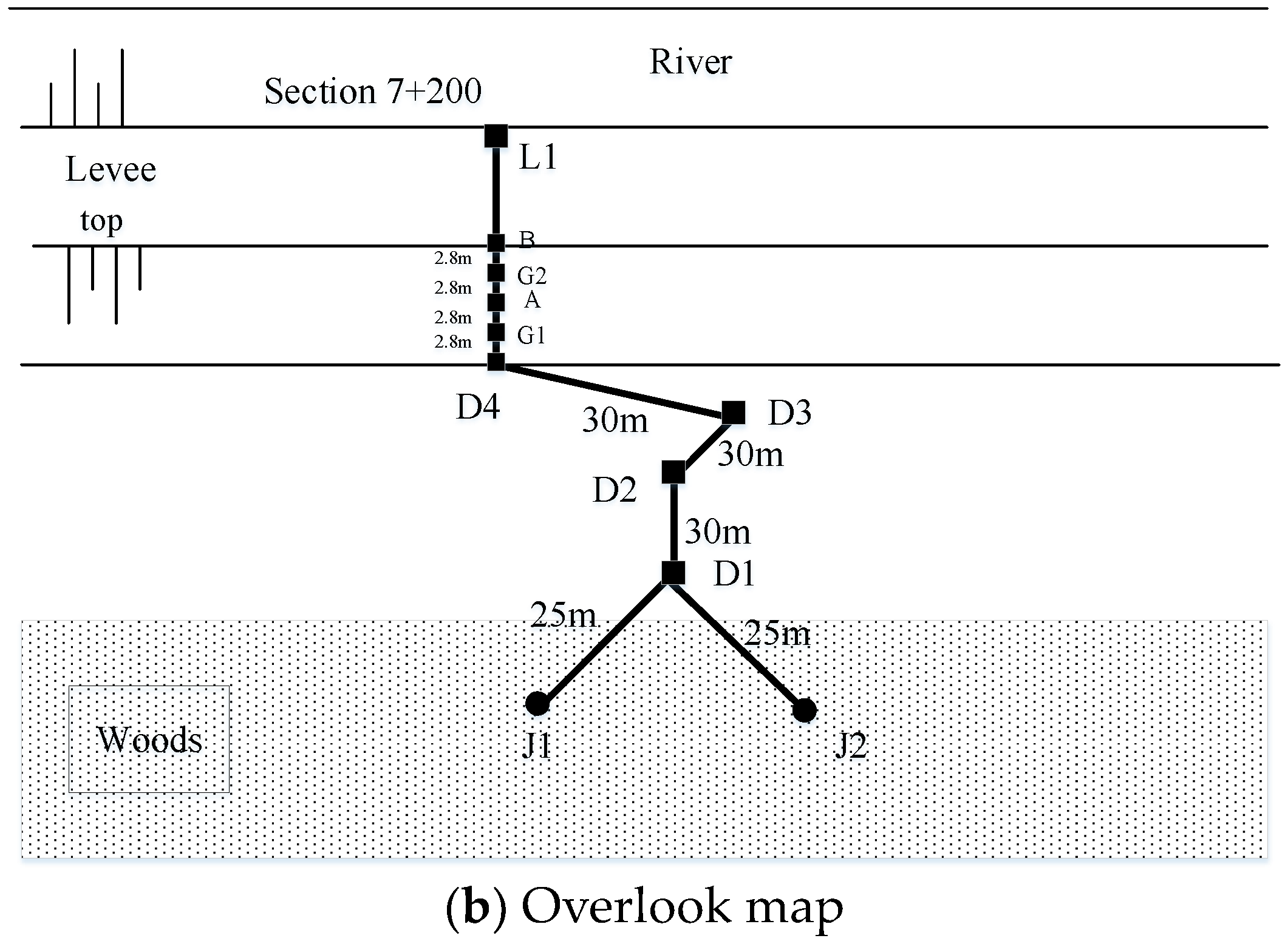
The measuring points layout for the HTL are shown in Figure 8. The points (L1, B, G2, A, G1, D4) were used for ground settlement measurement. The points (1–6) were used for internal settlement measurement.

3.1.4. Installation Process of Internal Settlement Observation

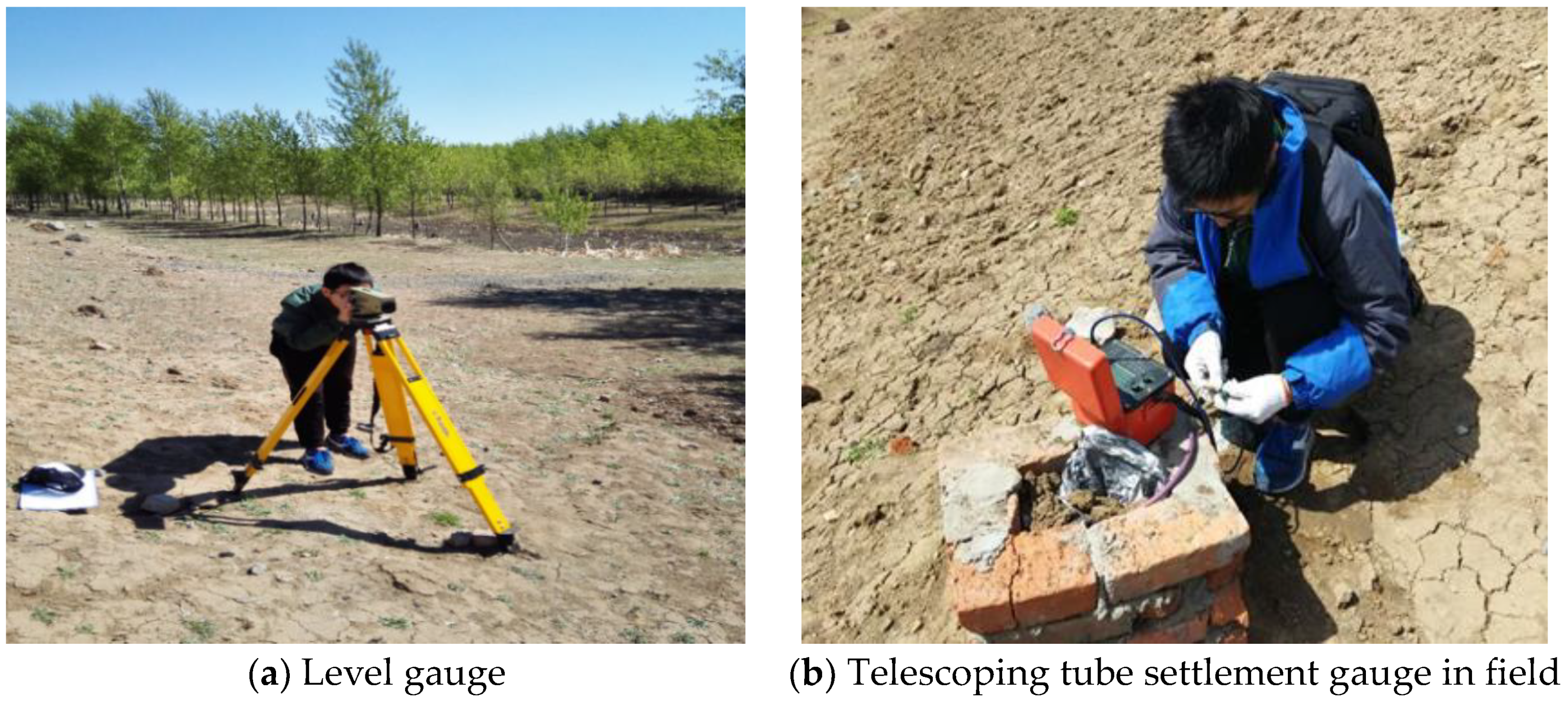
The leveling observation and internal settlement observation methods used in this study are shown in Figure 9. The specific installation process of the internal settlement observation was as follows:

(1)

The single end anchor head was installed at the deepest position;

(2)

The both ends anchor head was installed at the middle position. The differences between single end anchor head and both ends anchor head is the number of pipelines. The single end anchor head has no pipeline outlet, so it was installed at the deepest position;

(3)

The third step was to connect the pedestal and displacement sensor. The most important consideration in this step is the corresponding relationship between the serial number of displacement sensors and the position of the anchor head, as the displacement sensor and the anchor head will be buried in the HTL;

(4)

The fourth step was to assemble the pedestal. In this step, all displacement sensors were installed in the pedestal. The pedestal is the only instrument that will be outside the levee;

(5)

The fifth step was to assemble all anchor heads using a hydraulic pipe and plastic pipe. The aim of the hydraulic pipe was to transport hydraulic oil. The aim of the plastic pipe was to make every anchor head reach the right depth;

(6)

The sixth step was to inflate the oil hydraulic pump (pressure approximately 3–4 MPa) using hydraulic oil. After that, the all instruments can be placed into the hole;

(7)

The paws of all anchor heads were reduced. The aim of inflating the oil hydraulic pump was to shrink the paws of all anchor heads;

(8)

A hole was drilled on the spot;

(9)

All instruments were transported to the spot. Transportation in this step required several people because the instruments are very long;

(10)

All instruments were placed into the hole. The hydraulic pipe was to be cut off so that the paws of all anchor heads would be stuck into the hole wall;

(11)

Installation was completed.

(12)

The data collection is shown in Figure 9b.

The monitoring results are listed in

Table 5. Monitoring results unit: mm.

	Points	G1	A	G2	B	L1
Date
2016/11/3		0.00	1.20	−0.51	0.12	−0.51
2016/11/18		−0.51	−0.31	0.11	−0.15	−0.22
2016/12/3		−0.72	−0.52	−0.25	−0.39	−0.15
2016/12/18		−0.89	−1.21	−1.11	−0.61	−1.12
2017/1/2		−1.39	−1.18	−1.75	−0.78	−1.51
2017/1/17		−1.09	−1.50	−1.70	−0.58	−2.81
2017/2/1		−1.30	−1.49	−2.10	−3.60	−4.21
2017/2/15		−1.55	−1.48	−2.03	−3.63	−3.30
2017/3/1		−1.50	−1.43	−2.21	−4.98	−5.71
2017/3/16		−1.30	−1.61	−2.41	−5.23	−5.31
2017/3/31		−1.58	−1.80	−2.63	−6.10	−5.10
2017/4/15		−1.72	−1.50	−2.45	−5.87	−5.78
2017/5/1		−1.20	−1.68	−2.98	−6.23	−5.06
2017/5/15		−1.50	−1.79	−2.75	−5.12	−4.78
2017/5/31		−1.25	−1.48	−2.65	−5.29	−4.70
2017/6/15		−1.37	−1.51	−2.70	−5.23	−4.51
2017/7/1		−1.40	−1.60	−2.61	−5.33	−4.63

. The monitoring results provide basic data for settlement prediction.

3.2. Settlement Prediction Using GSPM

In this section, the GSPM is applied to describe the settlement rule of the HTL in order to validate its effectiveness. The specific method used is the curve fitting using Mathematica.

3.2.1. Application for Different Sections of HTL

In this section, the comparison with different sections using GSPM is discussed. Figure 10 provides the comparison with different sections of the HTL. The settlement comparison of the levee top demonstrated that the GSPM is suitable for the settlement prediction of the HTL.

The main reasons for the different settlement rules of the HTL are as follow: 1. The soils of different HTL sections are different; 2. The additional stress of different sections is different; 3. The environmental factors of different sections are different (for example, some sections may produce frost heave deformation). In particular, the S-shaped settlement–time curve from Section II is due to seepage deformation.

For Section I, the settlement stabilization time is approximately 100 days. In fact, monitoring data show that the settlement stabilization time is approximately 150 days. Moreover, the settlement stabilization times of the GSPM and hyperbolic models are close to the measured results. In terms of the final settlement prediction, the prediction results of the three models were basically consistent with the measured results. Hence, when the logistic model describes the hyperbolic settlement–time curve, it will result in an error of settlement stabilization time.

For Section II, the hyperbolic model is not convergent, which shows that the hyperbolic model is not suitable for predicting the S-shaped settlement–time curve. However, the predicted results of the GSPM and logistic models were basically consistent, which shows the validity of the GSPM in predicting the S-shaped settlement–time curve.

From the above analysis, the GSPM is effective and stable in predicting the hyperbolic and S-shaped settlement–time curves.

Table 6. Sum of squares of errors for different sections unit:mm².

Monitor Points	Prediction Models	Sum of Squares of Errors
Section I	GSPM	25.1
	Logistic model	35.5
	Hyperbolic model	27.9
Section II	GSPM	53.7
	Logistic model	55.5
	Hyperbolic model	99.1

presents the error analysis for different sections. The bold words in Table 6 represent the sum of squares of errors of GSPM, and it is also the minimum error of the three models, which demonstrate that the GSPM is suitable for the settlement prediction of an HTL.

3.2.2. Application for Specific Section of HTL

Ground Settlement Prediction

The ground settlement rules are given in Figure 11. The following conclusions can be drawn from Figure 11: 1. The settlement rules of different points show different shapes (S-type and hyperbolic); 2. The measured points at the foot of the slope show hyperbolic settlement, while the measured points on the top of the slope show S-type settlement; 3. The settlement stability time at the foot of the slope is shorter than that at the top of the slope; 4. The settlement of the top of the slope is larger than that at the foot of the slope. 5. The GSPM is applicable to settlement prediction, which is more stable than the hyperbolic model and logistic model.

Because of stress diffusion, the additional stress at the foot of the HTL is less than that at the top of the HTL, which explains why the deformation at the corner of the HTL is less than that at the top of the HTL.

Because the HTL is located in a seasonal freezing and thawing area, the temperature in winter can reach −30 °C. Under winter rainfall, soil at the top of the HTL is easily frozen, and the settlement of the HTL decreases with the increase of strength. After the ice and snow melts, the soil particles are rearranged, resulting in thaw settlement [37,38] and accelerated settlement. Therefore, the role of frozen soil in a seasonal freezing and thawing area can explain the S settlement rules at the top of the HTL.

For monitoring points G1 and A, the settlement–time curve is hyperbolic, as seen from Figure 11. From monitoring point A, the logistic model has the same problem for predicting the settlement stabilization time. For the final settlement prediction, the results from the logistic model are less accurate than those from the other two models.

There are three conclusions based on monitoring points G2, B, and L1: 1. The hyperbolic model is not suitable for predicting, which is consistent with Section 3.2.1; 2. Both the logistic model and the GSPM are suitable for predicting an S-shaped settlement–time curve; 3. For small settlements (0–3 mm), the logistic model can reduce the settlement stabilization time.

The GSPM can be more widely used, more accurate, and more stable than the traditional logistic model and hyperbolic model.

Internal Settlement Prediction

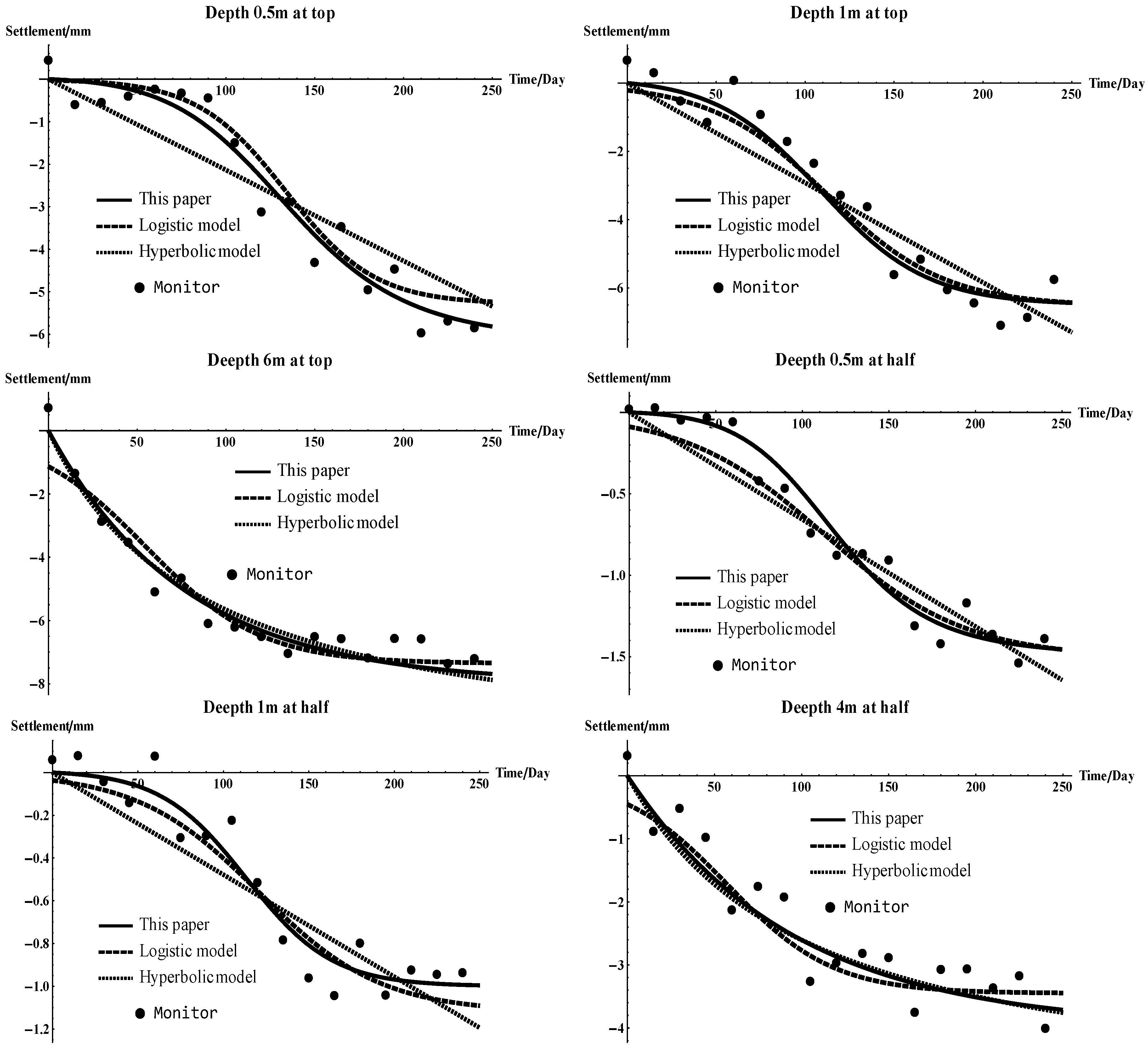
The rules of internal settlement of the HTL are given in Figure 12. The following conclusions can be drawn from Figure 12: 1. Settlements within 1 m of the top of the HTL tend to be S-shaped, while those below 4 m of the depth of the HTL tend to be hyperbolic; 2. The GSPM is also applicable in describing the law of internal settlement of the HTL. Moreover, the GSPM is more stable than the logistic model and hyperbolic model; 3. The internal settlement of the HTL is more than that of the top.

Similarly, owing to the influence of frozen soil at surface, the settlement of the soil near the surface appears S-shaped. Because the residents around the monitoring section have the habit of pumping groundwater, the descent of groundwater will cause internal settlement [6,39,40].

Table 7. Sum of squares of errors for different settlement–time models unit:mm².

Monitoring Points	Prediction Models	Sum of Squares of Errors
G1	GSPM	0.32
	Logistic model	0.34
	Hyperbolic model	0.4
A	GSPM	0.43
	Logistic model	0.65
	Hyperbolic model	0.81
G2	GSPM	0.93
	Logistic model	1.36
	Hyperbolic model	1.53
B	GSPM	3.71
	Logistic model	4.48
	Hyperbolic model	10.20
L	GSPM	4.43
	Logistic model	4.90
	Hyperbolic model	11.91
Depth 0.5 m at top	GSPM	3.93
	Logistic model	5.30
	Hyperbolic model	12.37
Depth 1 m at top	GSPM	5.89
	Logistic model	6.70
	Hyperbolic model	13.15
Depth 6 m at top	GSPM	4.02
	Logistic model	7.36
	Hyperbolic model	4.53
Depth 0.5 m at half	GSPM	0.22
	Logistic model	0.30
	Hyperbolic model	0.42
Depth 1 m at half	GSPM	0.19
	Logistic model	0.29
	Hyperbolic model	0.51
Depth 4 m at half	GSPM	2.68
	Logistic model	3.07
	Hyperbolic model	2.87

lists the sum of squares of errors of different models. The bold words in Table 7 represent the sum of squares of errors of GSPM, and it is also the minimum error among the three models, which shows that GSPM is more stable and adaptable than the logistic model and hyperbolic model. That’s because the GSPM has more parameters. Hence, the new model needs more data to fit.

3.3. Differential Settlement Control Criterion

Although the settlement was predicted in the previous section, the relationship between the predicted settlement and pavement cracking is still unknown. This will lead to uncertainty in the settlement control. Hence, the settlement control criterion will be discussed in the following section.

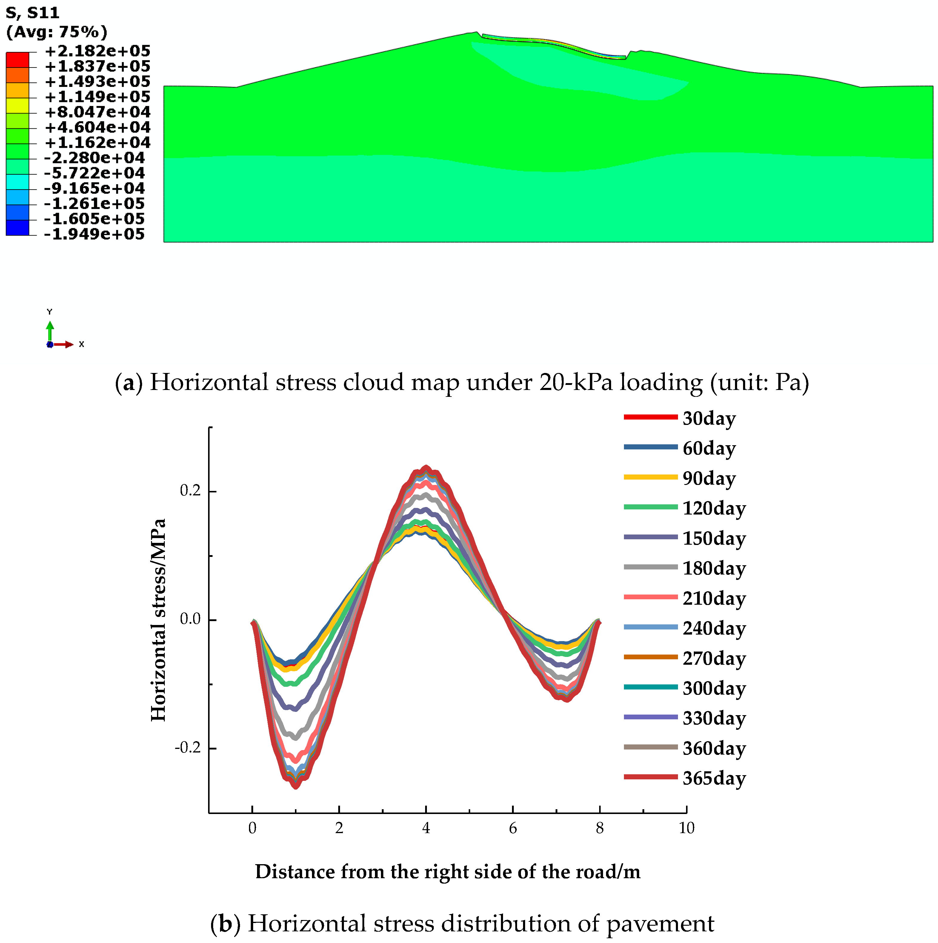
3.3.1. Horizontal Stress of Pavement

Figure 13 shows the horizontal stress distribution of pavement at the top of the HTL. The pavement cracking is caused by the horizontal tensile stress exceeding the ultimate tensile strength. Therefore, the horizontal stress distribution of the pavement is a very important factor to prevent pavement cracking.

From Figure 13a, it can be seen that the maximum horizontal tensile stress appears at the junction of the backfill and the old levee, which is basically consistent with the crack location in the actual project.

The main reason for pavement cracking is the compressibility difference between the backfill and the old levee owing to the insufficient compaction of backfill. This insufficient compaction of backfill may come from rolling during construction.

The time–space relationship of the horizontal stress of the pavement is shown in Figure 13b. It can be seen from Figure 13b that the horizontal stress of the pavement presents an asymmetric W-type in space. The horizontal stress on one side of the old levee is lower than that on the side of backfill, and the maximum tensile stress appears at the joint of the backfill and the old levee.

3.3.2. Relationship between Horizontal Stress of Pavement and Differential Settlement of HTL

Figure 14 gives the relationship between the horizontal stress and differential settlement under different load conditions. As mentioned above, the reason for pavement cracking is that the horizontal tensile stress exceeds the ultimate tensile stress. Hence, the horizontal tensile stress of the pavement is a very important factor to control pavement cracking. Based on Figure 14, when asphalt concrete pavement (the ultimate tensile stress is 0.12 MPa) is used, the corresponding differential settlement criterion is approximately 4.3 cm.

In fact, the differential settlement of the HTL is inevitable. Objectively, differential settlement that does not cause pavement cracking and reduces stability should be acceptable. A differential settlement control criterion can define how much differential settlement needs to be controlled, which is of great significance to guide engineering construction. Specifically, the settlement prediction value should be compared with the settlement control criterion. If the settlement prediction value is higher than the settlement control criterion, this section needs to be controlled.

The control criterion of differential settlement is common in expressway widening projects [41,42]. Yue-Dong et al. [41] proposed that the postconstruction settlement of the embankment of an expressway splicing section should not exceed 10 cm. Here, 10 cm is the control criterion. Yang En Hui [42] proposed a settlement ratio of 2.3‰ as a control criterion for mountainous highways.

The differential settlement control criterion established in this study is not constant, which is the main difference from previous studies [41,42]. The reasons are as follow: 1. The main cause of pavement cracking is differential settlement rather than uniform settlement, so it is not appropriate to use final settlement as the control criterion; 2. Pavement cracking is related to the tensile strength of the pavement structure. The ultimate tensile strength of different pavements is different. Therefore, differential settlement criterion should not be constant. Thus, the differential settlement criterion should be a value relative to the ultimate tensile strength of the pavement.

4. Research Limitations

In this study, the pavement cracking problem of an HTL was explored, but there are still some shortcomings.

• In the finite element calculation, the deformation of the pavement was coordinated with the top of the HTL. However, the actual failure mode may also be the cavity between the road surface and the top of the HTL. The cavity may be caused by biological caves, scouring, and other factors. This kind of pavement stress distribution under cavity is not considered in this study.
• In this study, only the application of the generalized settlement prediction model in the HTL was verified, and the application of other projects needs further verification.

5. Conclusions

Aiming at the pavement cracking problem of an HTL, field monitoring and finite element analysis were employed to attain settlement prediction and a differential settlement control criterion. The main conclusions are as follow:

(1)

The monitoring data showed that an HTL presents S-shaped and hyperbolic settlement rules, and the settlement law within 1 m of the top tends to be S-shaped, while the settlement law inside the HTL tends to hyperbolic. The settlement law of the S-shape is related to frozen soil. The rule of hyperbolic settlement is related to the decline of groundwater level.

(2)

A GSPM based on field monitoring data of an HTL was proposed. The effectiveness of the GSPM is validated from the point of view of engineering applications. The physical meanings of model parameters are analyzed. The GSPM proposed in this paper can be more widely used, more accurate, and more stable than the traditional logistic model and hyperbolic model.

(3)

The quantitative relationship between differential settlement and the horizontal stress of pavement is revealed using the finite element method. The maximum horizontal tensile stress appears at the junction of the backfill and the old levee, which is basically consistent with the crack location in the actual project. On this basis, the differential settlement control criterion for different pavements can be suggested. For example, when asphalt concrete pavement is used (whose ultimate tensile stress is 0.12 MPa), the corresponding differential settlement criterion is approximately 4.3 cm.

In the end, a differential settlement control method for an HTL is also a question worth studying in the future.