An Improved Empirical Wavelet Transform and Its Applications in Rolling Bearing Fault Diagnosis

Abstract

As essential but easily damaged parts of rotating machinery, rolling bearings have been deeply researched and widely used in mechanical processes. The real-time detection of bearing state and simple, rapid, and accurate diagnosis of bearing fault are indispensable to the industrial system. The bearing’s inner ring and outer ring vibration acceleration can be measured by high-precision sensors, and the running state of the bearing can be effectively extracted. The empirical wavelet transform (EWT) can adaptively decompose the vibration acceleration signal into a series of empirical modes. However, this method not only runs slowly, but also causes inexplicable empirical modes due to the unreasonable boundaries of the frequency domain division. In this paper, a new method is proposed to improve the empirical wavelet transform by dividing the boundaries from the spectrum, named the fast empirical wavelet transform (FEWT). The proposed method chooses different points in the Fourier transform of the spectrum (key function) to reconstruct the trend component of the spectrum. The minimum points in the trend component divide the spectrum into a series of bands. A more reasonable set of boundaries can be found by choosing appropriate trend components to obtain effective empirical modes. The simulation results show that the proposed method is effective and that the acquired empirical mode is more reasonable than the EWT method. Combining kurtosis with fault feature extraction of inner and outer rings of bearings, the method is successfully applied to the fault diagnosis of rolling bearings.

1. Introduction

Mechanical automation occupies a dominant position in modern industrial systems. Rotary machinery and bearings are indispensable to high-speed rail, intelligent robots, manipulators, and large-scale equipment production lines. In many cases, bearings may be subjected to high speed and a heavy load and may also face complicated conditions such as high and low-temperature differences. Even if the bearing structure is very delicate, it is difficult to tolerate a too-complex working environment for a long time. Sometimes minor damage can spread undetected, causing damage to the bearing and thus affecting the operation of the equipment. Healthy bearings are the basis for the normal operation of the equipment. Bearings that are prone to damage and breakdown are also one of the greatest hidden dangers that lead to equipment failure [1]. It can be seen that it is necessary to monitor and diagnose bearing faults.

With the popularization of mechanical automation and industrial intelligence, fewer people participate in the operation and management of equipment [2]. Real-time state-monitoring systems can compensate for the safety problems caused by manpower shortages. By monitoring the running state of mechanical equipment and collecting vibration acceleration signals of vulnerable parts, abnormal equipment can be found in time. When rotating machinery fails, the position deformation of the fault will lead to repeated collisions and periodic impact [3]. Extracting the components containing the impact information in the signal can improve the speed and accuracy of the diagnosis. Many scholars have studied methods of diagnosing vibration acceleration signals, such as short-time Fourier transform (STFT), Wigner–Ville distribution, and wavelet transform (WT) [4,5]. The window function of STFT cannot be adaptively adjusted according to the characteristic frequency of the signal itself, Wigner–Ville distribution generates cross-terms when processing signals with multiple frequency components and wavelet analysis (including continuous wavelet transform, discrete wavelet transform, dual-tree complex wavelet transform, etc.) [4] requires manual selection of wavelet basis functions and lacks self-adaptability. Empirical mode decomposition (EMD), proposed by Huang [6], can adaptively decompose a signal into a finite number of intrinsic mode functions (IMFs). These contain local features of different time scales in the original signal. However, the problems of modal aliasing, endpoint effect, and over envelope seriously affect the further development of EMD [7,8]. In order to avoid modal aliasing and weaken the endpoint effect to a certain extent, Gilles [9] proposed extracting modal information from the spectrum via empirical wavelet transform (EWT). The method is adaptive and reliable in the mathematical derivation. First, the Fourier spectrum is divided adaptively. Then the wavelet filter banks are set up to extract multiple single components with tightly supported Fourier spectra. Finally, the Hilbert transform is used to get instantaneous frequency and amplitude for each component. With these advantages, the EWT method was used to extract fault information from rolling bearings [10,11] and wind turbines in [12]. Real-time monitoring of power quality has also been widely promoted [13]. By comparing EMD, Ensemble EMD, EWT, and other methods, Kedadouche [14] and others came to the conclusion that the EWT method can effectively reveal the frequency and associated harmonics of faulty bearings.

Some new problems were discovered in the process of using EWT to extract faults. For example, the setting of parameters is usually difficult and the calculation is time-consuming [15], the unreasonable division of the spectrum will lead to unsatisfactory noise reduction [16] or decomposition of too many invalid components [17], and so on. After consulting the literature, authors have divided the methods of optimizing EWT into three categories. The first category is processing the empirical modes (EMs) obtained. This includes removing noise and combining empirical modes by calculating relevant indicators. Empirical modes reduce their own noise through the selection of mutual information; the reconstructed signals are used to combine the ambiguity function and correlation coefficients for ambiguity correlation classification (ACC). Finally, new signals are input into the ACC for testing and training [16]. Pan [18] and Song [19] calculated the Pearson’s correlation coefficient of the envelope spectrum of each empirical mode. By comparing the coefficients of these modes and combining the empirical modes below the standard, a slightly smaller empirical mode can be obtained. This process combines noise modes and reduces the number of empirical modes. Mingtao [20,21] calculated root mean square, kurtosis, and skewness of each empirical mode and combined them into feature vectors; kernel density estimation (KDE) and mutual information (MI) are combined to estimate classification feature vectors to diagnose faults. Correlation coefficients among empirical modes are calculated to extract more valuable components; the instantaneous amplitude was extracted by HT and STFT and the damage was characterized [22]. In view of the inconvenience of EWT spectrum segmentation caused by noise, Fourier–Bessel series expansion (FBSE) is mentioned to enhance spectrum and reduce noise; the scale–space method is used to split the FBSE spectrum [23]. This method suppresses the noise to some extent, but does not solve the problems of mode aliasing and invalid components caused by the scale–space method in EWT. Similarly, Luo [24] used the autoregressive power spectrum instead of the Fourier spectrum to divide boundaries; then, the boundaries were computed by the Burg algorithm to correct EWT. This approach also enhances the spectrum and reduces noise, but does not explain how to divide the boundaries in signals containing modulation components. This category adds more work on the premise that EWT takes more time. It takes a lot of time not only to set the initial parameters of EWT, but also to set the merge criteria. This will only make the algorithm more complicated. Although the noise is reduced to some extent, or the number of empirical modes is reduced, it does not change the defect of the EWT method itself. Therefore, it is necessary to improve the algorithm. The second category is optimizing the adaptability of EWT. Due to the disturbance of too many initial parameters, Zheng [15] proposed an adaptive parameterless empirical wavelet transform method. This method uses Otsu and K-means to segment the spectrum and establishes a set of adaptive bandpass filters to decompose the signal into mono-components with a compactly supported spectrum. Another adaptive method uses sparsity functions, first prewhitening the signal by using an autoregressive model, then automatically determining Fourier segments to conduct EWT and square envelope analysis [25]. Otsu and K-means methods have poor effects on spectrum segmentation; sparsity guide EWT needs to change parameters according to fault characteristics while optimizing parameters. The third category is optimizing spectrum segmentation. Hu [17,26] proposed a new method of spectrum segmentation, which uses an order statistical filter (OSF) to estimate the upper envelope function of the spectrum; by selecting the useful flat top in the upper envelope, the boundaries are determined to construct the filter and reconstruct the empirical modes. OSF is very effective in estimating envelope function, but the author did not point out how to get the best envelope function. Therefore, the method is not self-adaptive. Juan [27] used multiple signal classification to calculate the spectrum, which zeroes the part considered as noise and enlarges the part deemed useful. On the one hand, using multiple signal classification to calculate the spectrum of signals can reduce noise; on the other hand, it can amplify useful information while weakening the irrelevant information, so as to facilitate the division. In Reference [28], the natural frequencies are used as useful frequencies to calculate the support boundaries and decompose the signal into multiple components; kurtosis is used to automatically filter defect-related components and envelopes to extract characteristic frequency. However, the above three methods have certain limitations: the noise interference is very obvious when calculating the signal spectrum, and how to distinguish the strong noise from the signal needs to be further explored. Calculating the cutoff frequency and initializing the boundary with the type of fault needs to be performed; the final boundaries are determined by an iterative backward forward search algorithm, and MFMindex-aided adaptive Fourier spectrum segmentation is realized [29]. The multilevel EWT method proposed by Ding [30] simplifies the rules for splitting the spectrum. A multilevel boundary array is constructed based on the rotational frequency, outer race fault characteristic frequency, inner race fault characteristic frequency, roller fault characteristic frequency, and cage fault characteristic frequency and used for filtering and reconstruction. This method provides a complete framework for splitting the spectrum without depending on the characteristics of the spectrum. However, because of the difference between roller fault and inner ring fault characteristic frequencies, the decomposition level will be different. Self-adaptability is improved, while computing time is wasted. More invalid modes are extracted from each level. Therefore, optimizing the core of the EWT algorithm—segmentation of the spectrum—has become the focus of this research.

In this paper, a fast empirical wavelet transform is proposed. Based on the waveform characteristics of the spectrum, the problem of spectrum segmentation in EWT is improved. The trend of the spectrum is reconstructed from the Fourier function of the spectrum, and the minimum points of the trend are calculated as the boundaries. Different frequency components in the key function can reconstruct different trend components. By comparing the success rate and error rate of separation, it is proved that the boundaries of the fast empirical wavelet transform (FEWT)method are more reasonable. The experimental results show that the method is effective in the analysis of rolling bearing fault diagnosis. The method of dividing boundaries based on the Fourier transform function of the spectrum is not only fast but also self-adaptive, and can be effectively applied to online fault diagnosis systems. The structure of this paper is as follows: Section 2 briefly introduces EWT and its shortcomings; Section 3 elaborates the proposed FEWT method in detail and introduces the trend estimation method based on key function and threshold denoising; Section 4 uses three kinds of simulation signals to prove that the trend estimation method can obtain more reasonable boundaries and extract useful information effectively; and Section 5 combines kurtosis and fast kurtogram to verify the validity of the method through the fault of outer and inner rings of rolling bearings.

2. Exposition of Traditional EWT Method

2.1. EWT Method

The EWT method can be described by the following three steps: (1) adaptively segment the spectrum; (2) construct a suitable empirical wavelet filter bank according to the boundaries and filter the signal; and (3) reconstruct empirical modes and use Hilbert transform to demodulate and analyze.

Step 1: Divide the boundaries in the frequency domain.

The frequency domain of the signal is normalized to $\left[0,\mathsf{\pi }\right]$ and divided into $\mathrm{N}$ frequency bands with different bandwidths. Let $\mathsf{\omega }$ be the boundary between the bands; the left boundary is ${\mathsf{\omega }}_0=0$, the right boundary is ${\mathsf{\omega }}_{\mathrm{N}}=\mathsf{\pi }$, and the remaining boundaries can be expressed as ${\mathsf{\omega }}_1,{\mathsf{\omega }}_2,\dots ,{\mathsf{\omega }}_{\mathrm{N}}$, then each frequency band can be recorded as ${\mathsf{\Lambda }}_{\mathrm{n}}=\left[{\mathsf{\omega }}_{\mathrm{n}-1},{\mathsf{\omega }}_{\mathrm{n}}\right],\mathrm{n}=1,2,\dots ,\mathrm{N}$. It is obvious that ${{\displaystyle \cup }}_{\mathrm{n}=1}^{\mathrm{N}}{\mathsf{\Lambda }}_{\mathrm{n}}=\left[0,\mathsf{\pi }\right]$. With each boundary as the center, a transition phase with a width of ${\mathrm{T}}_{\mathrm{n}}=2{\mathsf{\tau }}_{\mathrm{n}}$ is defined for building a window base.

In this paper, the spectral trend estimation method based on the key function is used to obtain the boundary of each frequency band; instead of the method used by Gilles, the midpoint of the adjacent maxima is used as the boundary condition, as shown in Section 3.1.

Step 2: Construct an empirical wavelet filter bank.

The Meyer wavelet was selected by Gilles as a basis function to construct an empirical wavelet. A group of mutually orthogonal trigonometric functions is designed in the transition phase where the boundary of the frequency band is located, and a constant is designed in the frequency band. The empirical scaling function ${\varnothing }_{\mathrm{n}}\left(\mathsf{\omega }\right)$ and the empirical wavelets ${\mathsf{\Psi }}_{\mathrm{n}}\left(\mathsf{\omega }\right)$ can be defined as

$${\widehat{\varnothing }}_{\mathrm{n}}\left(\mathsf{\omega }\right)=(\begin{array}{c}1;\left|\mathsf{\omega }\right|\le \left(1-\mathsf{\gamma }\right){\mathsf{\omega }}_{\mathrm{n}}\\ \cos \left[\frac{\mathsf{\pi }}{2}\mathsf{\beta }\left(\frac{1}{2{\mathsf{\gamma }\mathsf{\omega }}_{\mathrm{n}}}\left(\left|\mathsf{\omega }\right|-\left(1-\mathsf{\gamma }\right){\mathsf{\omega }}_{\mathrm{n}}\right)\right)\right]\\ 0; \mathrm{others}\end{array};\left(1-\mathsf{\gamma }\right){\mathsf{\omega }}_{\mathrm{n}}\le \left|\mathsf{\omega }\right|\le \left(1+\mathsf{\gamma }\right){\mathsf{\omega }}_{\mathrm{n}}$$

(1)

$${ \widehat{\mathsf{\Psi }}}_{\mathrm{n}}\left(\mathsf{\omega }\right)=(\begin{array}{c}1;\left(1+\mathsf{\gamma }\right){\mathsf{\omega }}_{\mathrm{n}}\le \left|\mathsf{\omega }\right|\le \left(1-\mathsf{\gamma }\right){\mathsf{\omega }}_{\mathrm{n}+1}\\ \cos \left[\frac{\mathsf{\pi }}{2}\mathsf{\beta }\left(\frac{1}{2{\mathsf{\gamma }\mathsf{\omega }}_{\mathrm{n}+1}}\left(\left|\mathsf{\omega }\right|-\left(1-\mathsf{\gamma }\right){\mathsf{\omega }}_{\mathrm{n}+1}\right)\right)\right];\left(1-\mathsf{\gamma }\right){\mathsf{\omega }}_{\mathrm{n}+1}\le \left|\mathsf{\omega }\right|\le \left(1+\mathsf{\gamma }\right){\mathsf{\omega }}_{\mathrm{n}}\\ \sin \left[\frac{\mathsf{\pi }}{2}\mathsf{\beta }\left(\frac{1}{2{\mathsf{\gamma }\mathsf{\omega }}_{\mathrm{n} }}\left(\left|\mathsf{\omega }\right|-\left(1-\mathsf{\gamma }\right){\mathsf{\omega }}_{\mathrm{n}+1}\right)\right)\right]; \left(1-\mathsf{\gamma }\right){\mathsf{\omega }}_{\mathrm{n}}\le \left|\mathsf{\omega }\right|\le \left(1+\mathsf{\gamma }\right){\mathsf{\omega }}_{\mathrm{n}} \\ 0; \mathrm{others}\end{array}$$

(2)

where the transition function $\mathsf{\beta }\left(\mathrm{x}\right)$, the coefficient $\mathsf{\gamma }$, and the transition phase ${\mathsf{\tau }}_{\mathrm{n}}$ are

$$\mathsf{\beta }\left(\mathrm{x}\right)={\mathrm{x}}^4\left(35-84\mathrm{x}+70{\mathrm{x}}^2-20{\mathrm{x}}^3\right)$$

(3)

$$\mathsf{\gamma }<min\left(\frac{{\mathsf{\omega }}_{\mathrm{n}+1}-{\mathsf{\omega }}_{\mathrm{n}}}{{\mathsf{\omega }}_{\mathrm{n}+1}+{\mathsf{\omega }}_{\mathrm{n}}}\right)$$

(4)

$${\mathsf{\tau }}_{\mathrm{n}}={\mathsf{\gamma }\mathsf{\omega }}_{\mathrm{n}} , 0<\gamma <1$$

(5)

Step 3: Conduct an empirical wavelet transform.

The empirical wavelet transform ${\mathrm{W}}_{\mathrm{f}}^{\mathsf{\epsilon }}$ is defined by a method similar to the traditional wavelet transform, the Fourier transform is $\mathrm{F}(·)$, and the inverse Fourier transform is ${\mathrm{F}}^{-1}(·)$

$${\mathrm{W}}_{\mathrm{f}}^{\mathsf{\epsilon }}\left(\mathrm{n},\mathrm{t}\right)= \langle f\left(\mathrm{t}\right),{\mathsf{\Psi }}_{\mathrm{n}}\left(\mathrm{t}\right)\rangle ={{\displaystyle \int }}^{}\mathrm{f}\left(\mathsf{\tau }\right)\overline{{\mathsf{\Psi }}_{\mathrm{n}}\left(\mathsf{\tau }-\mathrm{t}\right)}\mathrm{d}\mathsf{\tau }={\mathrm{F}}^{-1}\left(\mathrm{f}\left(\mathsf{\omega }\right){ \widehat{\mathsf{\Psi }}}_{\mathrm{n}}\left(\mathsf{\omega }\right)\right)$$

(6)

Generate the approximation coefficients ${\mathrm{W}}_{\mathrm{f}}^{\mathsf{\epsilon }}\left(\mathrm{n},\mathrm{t}\right)$ by the inner product of the signal with the empirical scaling function:

$${\mathrm{W}}_{\mathrm{f}}^{\mathsf{\epsilon }}\left(0,\mathrm{t}\right)= \langle f\left(\mathrm{t}\right),{\varnothing }_1\left(\mathrm{t}\right)\rangle ={{\displaystyle \int }}^{}\mathrm{f}\left(\mathsf{\tau }\right)\overline{{\varnothing }_1\left(\mathsf{\tau }-\mathrm{t}\right)}\mathrm{d}\mathsf{\tau }={\mathrm{F}}^{-1}\left(\mathrm{f}\left(\mathsf{\omega }\right){\widehat{\varnothing }}_1\left(\mathsf{\omega }\right)\right)$$

(7)

where $\widehat{\mathrm{x}}\left(\mathsf{\omega }\right)$, ${\widehat{\varnothing }}_1\left(\mathsf{\omega }\right)$, ${ \widehat{\mathsf{\Psi }}}_{\mathrm{n}}\left(\mathsf{\omega }\right)$ can be expressed as Fourier transforms of $\mathrm{x}$, ${\varnothing }_1\left(\mathsf{\omega }\right)$, and ${\mathsf{\Psi }}_{\mathrm{n}}\left(\mathsf{\omega }\right)$. The signal can be rebuilt as follows:

$$\begin{gathered} \mathrm{f}\left(\mathrm{t}\right)={\mathrm{W}}_{\mathrm{f}}^{\mathsf{\epsilon }}\left(0,\mathrm{t}\right)\ast {\varnothing }_1\left(\mathsf{\omega }\right)+{\displaystyle \sum }_{\mathrm{n}=1}^{\mathrm{N}}{\mathrm{W}}_{\mathrm{f}}^{\mathsf{\epsilon }}\left(\mathrm{n},\mathrm{t}\right){\ast \mathsf{\Psi }}_{\mathrm{n}}\left(\mathrm{t}\right) \\ ={\mathrm{F}}^{-1}\left({ \widehat{\mathrm{W}}}_{\mathrm{f}}^{\mathsf{\epsilon }}\left(0,\mathsf{\omega }\right){\widehat{\varnothing }}_1\left(\mathsf{\omega }\right)+{\displaystyle \sum }_{\mathrm{n}=1}^{\mathrm{N}}{ \widehat{\mathrm{W}}}_{\mathrm{f}}^{\mathsf{\epsilon }}\left(\mathrm{n},\mathsf{\omega }\right){\mathsf{\Psi }}_{\mathrm{n}}\left(\mathsf{\omega }\right)\right) \end{gathered}$$

(8)

where ${\widehat{\mathrm{W}}}_{\mathrm{f}}^{\mathsf{\epsilon }}\left(0,\mathsf{\omega }\right)$ and ${ \widehat{\mathrm{W}}}_{\mathrm{f}}^{\mathsf{\epsilon }}\left(\mathrm{n},\mathsf{\omega }\right)$ can be expressed as Fourier transforms of ${\mathrm{W}}_{\mathrm{f}}^{\mathsf{\epsilon }}\left(0,\mathrm{t}\right)$ and ${\mathrm{W}}_{\mathrm{f}}^{\mathsf{\epsilon }}\left(\mathrm{n},\mathrm{t}\right)$. The empirical mode can be given by

$$\{\begin{array}{c}{\mathrm{f}}_0\left(\mathrm{t}\right)={\mathrm{W}}_{\mathrm{f}}^{\mathsf{\epsilon }}\left(0,\mathrm{t}\right)\ast {\varnothing }_1\left(\mathrm{t}\right)\\ {\mathrm{f}}_{\mathrm{k}}\left(\mathrm{t}\right)={\mathrm{W}}_{\mathrm{f}}^{\mathsf{\epsilon }}\left(\mathrm{n},\mathrm{t}\right)\ast {\mathsf{\Psi }}_{\mathrm{k}}\left(\mathrm{t}\right)\end{array}$$

(9)

After obtaining the empirical mode of the signal, the Hilbert transform can be used to calculate instantaneous frequency and instantaneous amplitude or to diagnose faults.

2.2. Drawbacks of the EWT Method

The key step in the process of an empirical wavelet transform is dividing the appropriate boundaries in the spectrum. When a large number of parameters are set up to achieve adaptive partitioning, it is difficult in most cases to obtain the appropriate boundary: (1) it is difficult to separate them when the spectra of different components are closer, which will lead to modal aliasing; and (2) when the signal-to-noise ratio (SNR) is low, the noise components cannot be eliminated and more invalid components will be obtained.

In Figure 1, the areas labeled A show that the two cosine signals with a relatively close frequency are not separated, and the area labeled B shows that the noise is divided into many ineffective components.

The adaptive method needs to set parameters: InitBounds. The initial boundary is difficult to determine, and the number of edges directly affects the results of segmentation. There are a number of types of split spectrum in scale–space, but they lead to too many invalid components in the frequency domain, as shown in B. Therefore, it is necessary to explore a fast and reasonable method to divide the boundaries from the spectrum to improve the empirical wavelet transform.

3. Proposed Method of Fast Empirical Wavelet Transform

In this paper, the above two defects of EWT are discussed and expounded: spectrum segmentation and boundary optimization. A new improved empirical wavelet transform method is proposed. This method obtains the trend component of the spectrum by obtaining the Fourier transform function (key function) of the spectrum. Minimum points of the trend component are used as boundaries to reconstruct the signal. Selecting different points in key functions will reconstruct different trend components. Suitable trend components can obtain reasonable boundaries for EWT. Figure 2 shows the process of the proposed method. The specific steps are as follows:

Step 1: Collect periodic impact signals $y\left(t\right)$. The fast Fourier transform (FFT) algorithm is used to acquire spectrum $Y\left(f\right)$. The Fourier transform function of $Y\left(f\right)$ is obtained through the FFT algorithm again, namely, the key function $K\left(f\right)$.

Step 2: A certain number of points in the key function are extracted to inverse the Fourier transform and reconstruct the trend component ($T_c\left(f\right)$) of the spectrum. When more points are used to reconstruct the complex trend component, the number of extreme points of the trend component will be larger, so that the spectrum will be divided into many parts. The reconstructed function is close to the trend of spectrum changes, and the spectrum will be partitioned into fewer parts. Section 3.1 describes the details of this method.

Step 3: Calculate the boundaries of the spectrum and optimize.

Taking the trend component as the basis function, the minimum point sequence is used as the boundary array. When the trend component is complex, the boundary array is optimized by the wavelet threshold. The method of optimizing spectrum boundaries based on threshold denoising reduces the invalid components caused by noise to a certain extent. This method will be introduced in Section 3.2.

Step 4: Perform signal processing using empirical wavelet transform.

The frequency domain of the signal is normalized to $\left[0,\mathsf{\pi }\right]$; choose Meyer wavelet as the basis function; define the empirical scaling function ${\mathsf{\varnothing }}_n\left(\mathsf{\omega }\right)$ and the empirical wavelets ${\Psi }_n\left(\mathsf{\omega }\right)$; build adaptive filters; decompose the signal into different components.

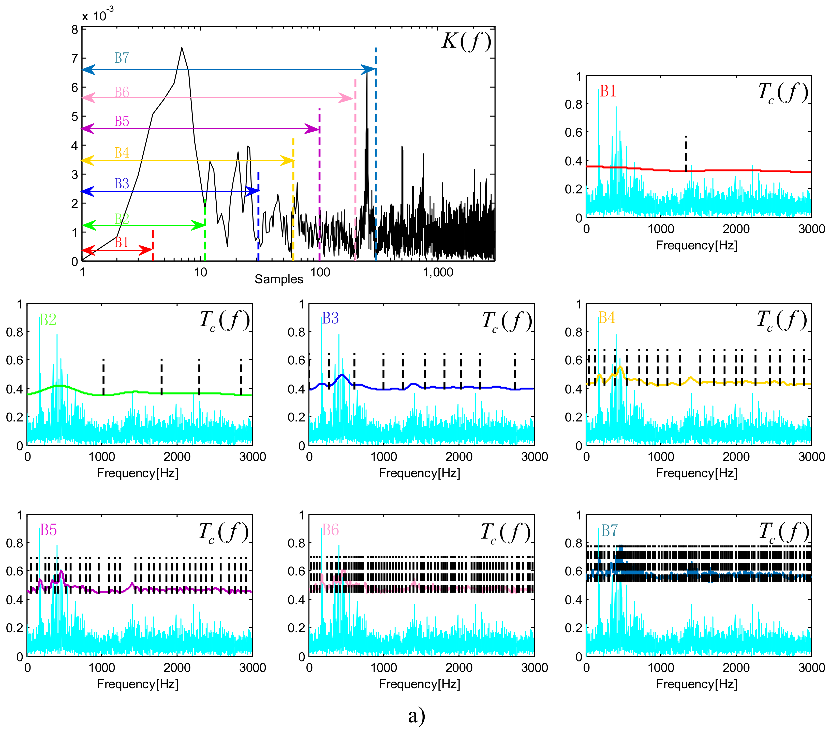
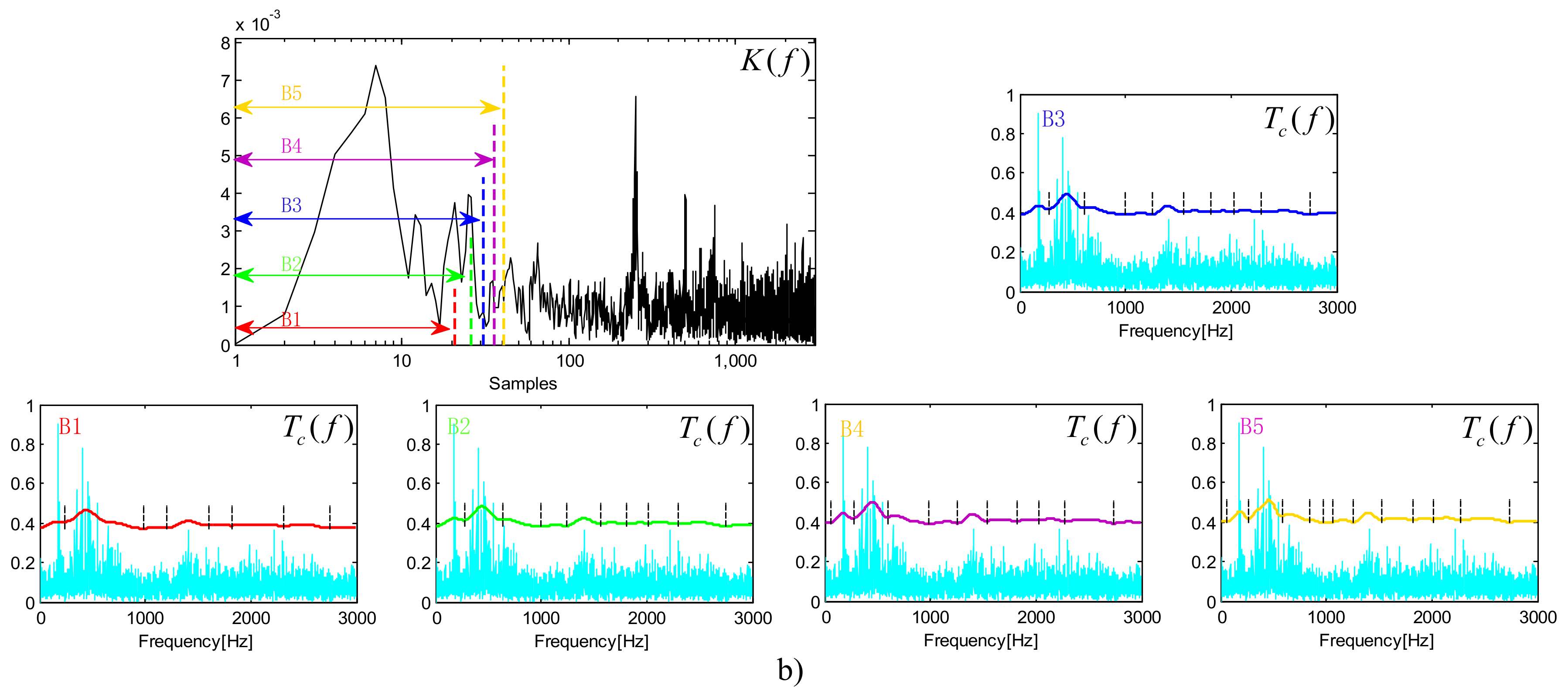
3.1. Trend Estimation Method Based on the Key Function

In the proposed method, the step of trend estimation based on the key function can be used to reconstruct the trend of the spectrum. This method inherits the theoretical basis of the Fourier transform. It is better than an interpolation algorithm in terms of computation time; the algorithm is more effective than the traditional empirical wavelet transform. Figure 3 shows the process of obtaining trend components.

Step 1: Obtain the spectrum of the measured signal using the FFT algorithm, as shown in Figure 3a.

$$Y\left(f\right)=FFT\left(y\left(t\right)\right)$$

(10)

Step 2: Calculate the Fourier transform function of $Y\left(f\right)$. Figure 3b,d show the key function.

$$K\left(f\right)=FFT\left(Y\left(f\right)\right)$$

(11)

Step 3: The components of key functions are closely related to the spectrum. Different functions can be obtained through low-pass filtering of key functions. The blue line in Figure 3c can be obtained by inverse FFT (iFFT) low-pass filtering with $\mathrm{B}1=30$ as the boundary. This blue line approximates the trend of the spectrum, called the trend component:

$$T_c\left(f\right)=iFFT\left(K_B\left(f\right)\right)$$

(12)

where $K_B\left(f\right)$ is the left part of boundary $\mathrm{B}$ in $K\left(f\right)$ and $T_c\left(f\right)$ is a trend component.

The purple line in Figure 3e can be obtained by inverse FFT low-pass filtering with $\mathrm{B}1=300$ as the boundary. Compared with the above results, it is obvious that different trend components can be reconstructed by inverse FFT with different frequency components. Therefore, it is necessary to study how the number of reconstructed points affects trend components.

It can be seen that as the number of reconstructed points increases, the trend components become more and more complex; different trend components will have different division results. When the number of reconstructed points is smaller than the first peak value of the key function, such as B1, the trend component is gentle and fluctuates very little, approximates a straight line, and cannot clearly be seen from the spectrum fluctuation trend. One minimum divides the spectrum into two areas. The first area contains a large amount of information and does not separate the corresponding frequency components in the spectrum. Thirty points are used to reconstruct the trend component (blue line), where the minimum values are regarded as the boundaries (black line). The key clusters in the spectrum are successfully extracted. Compared with the red line, the trend component corresponding to the blue line is divided into more bands, and the spectrum information contained in each band is more representative and readable. If the number of reconstructed points is increased to $\mathrm{B}5,\mathrm{B}6,\mathrm{B}7$, the trend component will become more complex and the number of minimum points will increase rapidly. The boundary divides the spectrum into more ineffective components. Comparing the seven trend components, the trend component can respond to the trend of spectral fluctuation when the number of reconstructed points is $\mathrm{B}3=30$. In order to accurately determine the optimal frequency component in the key function, the intervals of five frequency components are $\mathrm{B}1=20,\mathrm{B}2=25,\mathrm{B}3=30,\mathrm{B}4=35,\mathrm{B}5=40$. To calculate trend components, as in Figure 4b, on the premise of 20 points spanning the front and back, the trend components are almost the same; the boundary sequence of trend minima is also similar. Therefore, it is meaningless to find a more accurate frequency component; it allows the number of reconstructed points to fluctuate in a small range.

For signals with modulated components and bandwidth, it is necessary to estimate the trend to extract signals. The number of reconstructed points should be $\mathrm{B}\in \left[10,60\right]$. In Figure 1, for two signals whose spectra are close to each other, it is necessary to divide them accurately in order to extract the signals. Rolling bearings are one of the most easily damaged parts in rotating machinery. When a rolling bearing fails, the rolling body will impact periodically when it touches the fault position [31,32]. Shock information exists with modulating components but does not exist alone. The impact and modulation components show a cluster of modulation information containing a side band in the spectrum. How to extract the modulation information of each cluster becomes the most critical step in the process of splitting the spectrum. The vibration acceleration sensor is sensitive to impact information. Trend components represent the trend of spectrum change, and can better fit the similar modulation information, which may contain shock information in each cluster of the spectrum. Therefore, the trend estimation method based on the key function has advantages in dealing with rolling bearing fault diagnosis. The method based on FFT and iFFT is fast in calculating trend components. It has obvious advantages over the traditional EWT in dealing with analog signals (see Section 4) and practical signals (see Section 5). Choosing too few points from the key function for the inverse transformation will lead to rough partition that cannot distinguish the information with close frequency, but it can well contain the modulation information with side-band frequency. The proposed method can preserve and exclude the useless components to a certain extent. For simulation signals, when many points are selected for inverse transformation, some details can be extracted, such as the components whose spectra are close to each other, but this will cause the spectrum to be divided into too many areas. This paper proposes a threshold noise-reduction method to optimize the above problems.

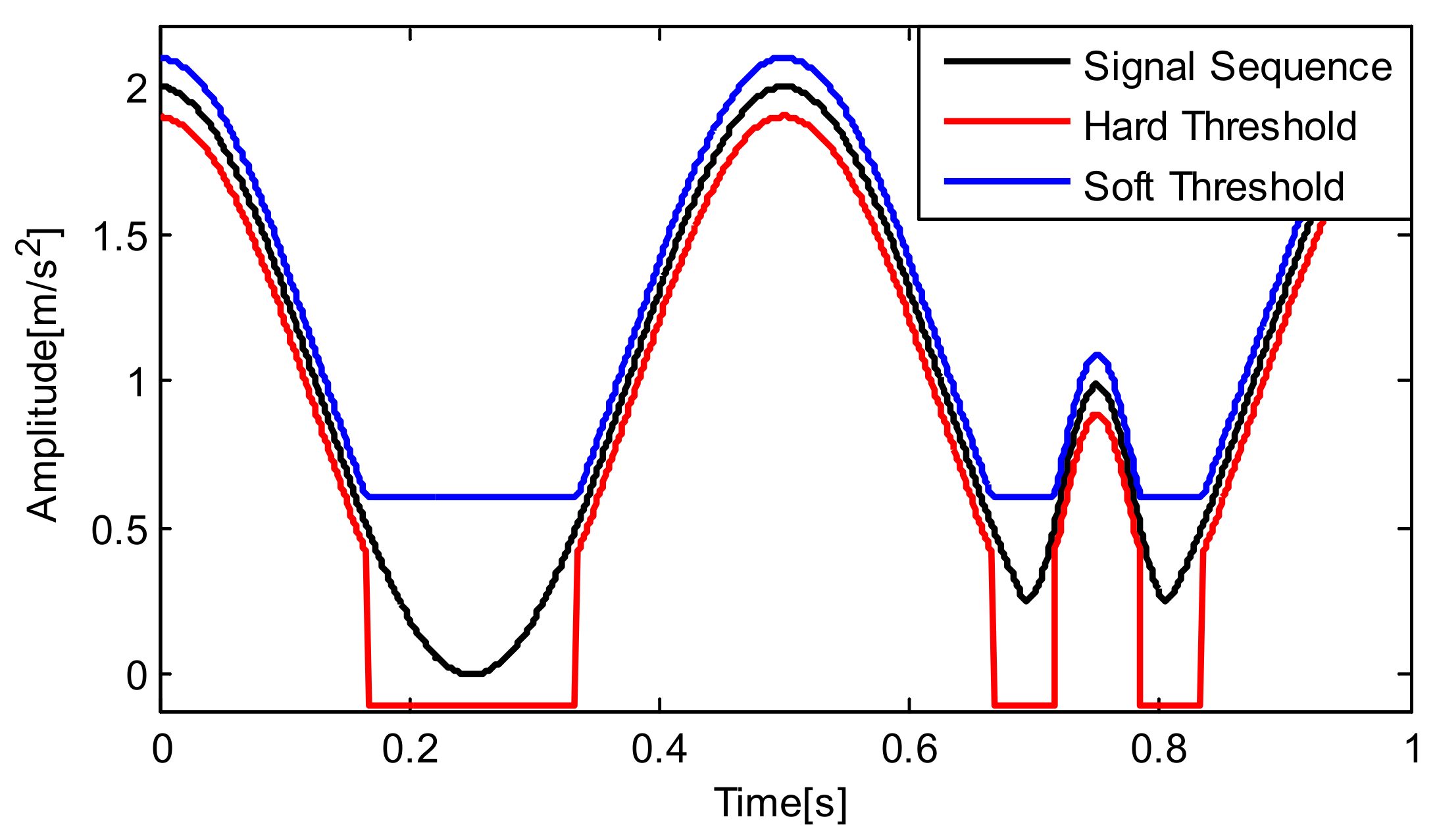
3.2. Threshold Denoising Method

Threshold denoising is mostly used for wavelet threshold denoising. After obtaining the wavelet coefficients through wavelet decomposition, the coefficients are denoised and the signals are reconstructed. In the process of threshold denoising, different threshold functions affect not only the denoising effect, but also the reconstruction results. It is critical to set the threshold when estimating data. Because this method does not need to show the trend completely, the spectrum fluctuation caused by noise needs to be reduced in the process of threshold denoising. Therefore, there is a certain fault tolerance when thresholds are obtained.

Commonly used threshold functions include the hard threshold function:

$$\widehat{\mathrm{s}}=\{\begin{array}{c}s \left|\mathrm{s}\right|\ge \lambda \\ 0 \left|\mathrm{s}\right|<\lambda \end{array}$$

(13)

and the soft threshold function:

$$\widehat{\mathrm{s}}=\{\begin{array}{c}\mathrm{sgn}\left(\mathrm{s}\right)·\left(\left|\mathrm{s}\right|-\lambda \right) \left|\mathrm{s}\right|\ge \lambda \\ 0 \left|\mathrm{s}\right|<\lambda \end{array}$$

(14)

where $\mathrm{s}$ is the signal to be processed and $\widehat{\mathrm{s}}$ is the signal after denoising.

Donoho and Johnstone [33] give the fixed threshold of $\mathsf{\lambda }$:

$$\mathsf{\lambda }=\mathsf{\sigma }\sqrt{2\ln \left(\mathrm{N}\right)}$$

(15)

where $\mathrm{N}$ is the length of the signal to be processed and ${\mathsf{\sigma }}^2$ is the estimated noise variance:

$$\mathsf{\sigma }=\mathrm{Mean}\left(\mathrm{s}\right)/0.6745$$

(16)

The hard threshold can preserve the local information of the signal very well in the processing, but the discontinuity of $\mathrm{s}$ at $\mathsf{\lambda }$ and $-\mathsf{\lambda }$ leads to oscillation of the reconstructed signal at the discontinuity point. The overall continuity of $\widehat{\mathrm{s}}$ is better during soft threshold processing. Although the derivatives are discontinuous and there is always a constant deviation between $\mathrm{s}$ and $\widehat{\mathrm{s}}$, which may affect the accuracy of reconstruction, this method only needs to obtain the spectrum trend and can ignore these defects of the soft threshold. Figure 5 shows the differences in noise reduction between the hard and soft threshold, where the black line is a signal sequence. The signal sequence is processed by using $\mathsf{\lambda }=0.5 \mathrm{m}/{\mathrm{s}}^2$ as the threshold. The red line is the result of a hard threshold; the blue line is the result of a soft threshold. It can clearly be seen from the graph that soft thresholds have a good continuity, while hard thresholds have local steps. In this paper, soft thresholds are used to process trend components.

4. Simulated Signal Verification

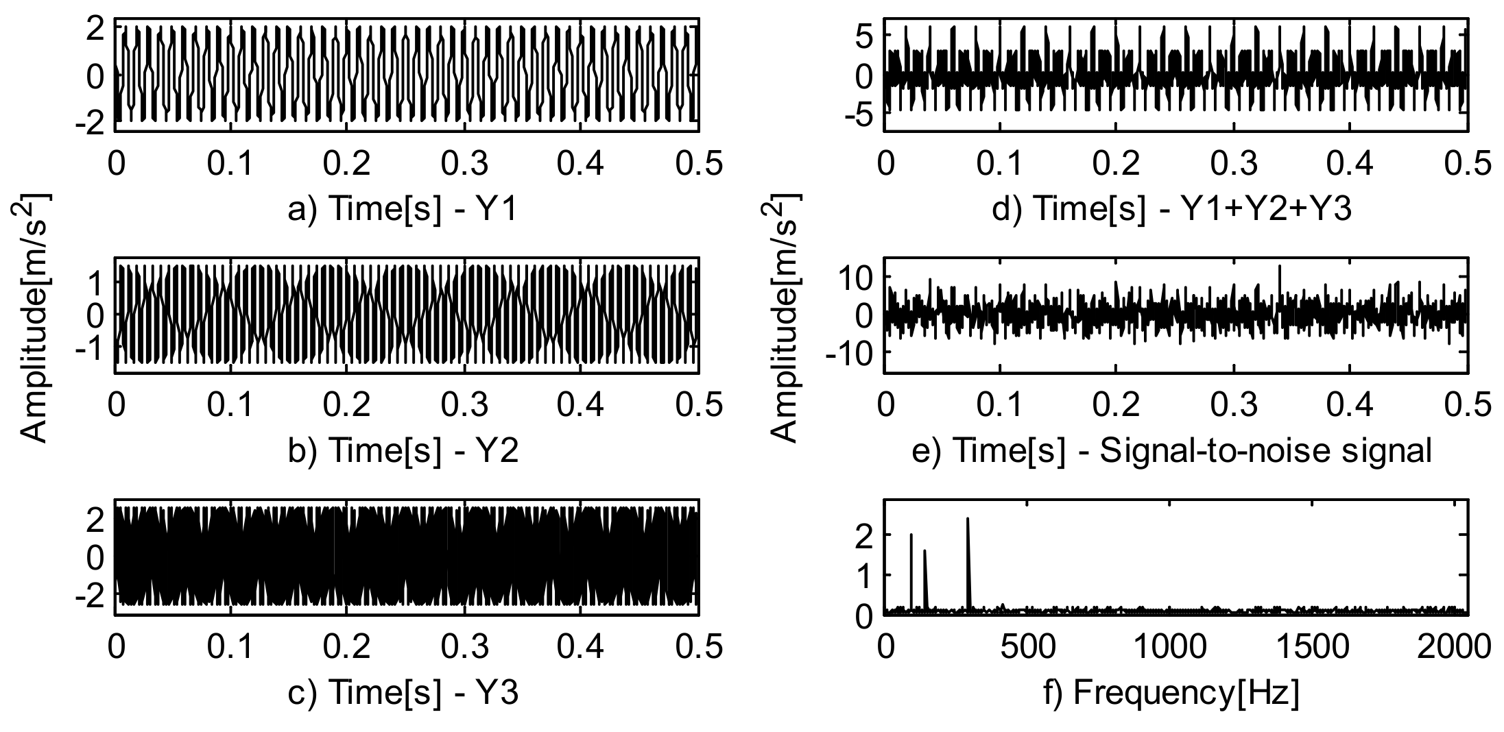
EWT needs to set many parameters when dividing boundaries, and different parameters will get different results. This affects its adaptability to some extent. The time required to repeatedly modify a large number of parameters exceeds the time saved by its self-adaptation. Sometimes it is difficult to distinguish two components whose frequencies are close. In a low signal-to-noise ratio signal, EWT divides more invalid components to bring unnecessary trouble to the analysis. In view of the above problems, three sets of simulation signals are given in this section to prove that FEWT boundary demarcation is more reasonable, faster, and more efficient than EWT.

4.1. Case Study 1

The first simulation signal consists of three cosine signals with different frequencies and amplitudes.

$$\{\begin{array}{c}{\mathrm{s}}_1=2.0\cos \left(2{\mathsf{\pi }\mathrm{f}}_1\mathrm{t}\right)\\ {\mathrm{s}}_2=1.5\cos \left(2{\mathsf{\pi }\mathrm{f}}_2\mathrm{t}\right)\\ {\mathrm{s}}_3=2.5\cos \left(2{\mathsf{\pi }\mathrm{f}}_3\mathrm{t}\right)\\ s={\mathrm{s}}_1+{\mathrm{s}}_2+{\mathrm{s}}_3+\mathsf{\eta }\end{array}$$

(17)

Among them, ${\mathrm{f}}_1=100 \mathrm{Hz}$; ${\mathrm{f}}_2=150 \mathrm{Hz}$; ${\mathrm{f}}_3=300 \mathrm{Hz}$; and $\mathsf{\eta }=\mathrm{SNR}\left(3\right)$.

The composition, noise, and spectrum of the simulation signal are shown in Figure 6. The signal contains three frequency components: $100 \mathrm{Hz}$, $150 \mathrm{Hz}$, and $300 \mathrm{Hz}$. The frequencies of the first two cosine signals are close to each other. How to successfully extract these three components and minimize the noise interference in the extracted components becomes an important problem to be solved.

First, the proposed EWT and FEWT methods are used to process the signals. Figure 7 shows the effect comparison of the two methods in terms of boundary segmentation. The long red dashed lines are the boundaries of FEWT and the short blue dashed lines are the boundaries of EWT. It can be seen from the figure that the blue boundaries divide the spectrum into too many areas. Although the components represented by ${\mathrm{f}}_3$ were successfully extracted, ${\mathrm{f}}_1$ and ${\mathrm{f}}_2$ were not distinguished. This is one of the biggest defects of EWT. Another major defect, dividing too many regions, will lead to the same amount of invalid components in the next reconstruction, which may increase the workload of the subsequent analysis and interfere with diagnosis. In the process of signal processing by the FEWT method, the first 180 points are selected from key functions to reconstruct trend components. After calculation, the soft threshold denoising process is $\mathsf{\lambda }=0.2309$. The minimum point in the trend component after noise reduction can be well separated into three frequencies and contains only a few unavoidable noises. In Figure 7, the regions divided by long red dashed lines are more reasonable than the short blue dotted lines.

Since EWT decomposes too many components, only the first three components of the EWT containing all three simulation signals are extracted for comparison. As shown in Figure 8a, the EWT method does not separate the components of $100 \mathrm{Hz}$, $150 \mathrm{Hz}$, and $300 \mathrm{Hz}$. There is modal aliasing in EM1, and EM2 is the component with a frequency of $300 \mathrm{Hz}$. However, because it contains more noise, it causes a very unstable modulation phenomenon. EM3 and the remaining components are invalid components that only contain noise. In the process of processing the signal by FEWT, under the effect of threshold noise reduction, the spectral boundary shrinks closer to the frequency of the component. The components representing the 2, 4, and 6 frequency domains are shown in Figure 8b. It can be seen from the figure that the three components are perfectly separated. The amplitudes of the three components have only a small fluctuation, which proves that the noise contained in the signal is small. It is proved that the proposed method is suitable for signals with relatively close frequencies. At this point, the FEWT method is superior to the EWT method.

For the simulation signal, this paper verifies the rationality of the FEWT boundary from two aspects: the success rate of separation and the error rate. The formula for the success rate of separation is as follows:

$$\mathrm{rate}\_\mathrm{Success}=\mathrm{effective}\left(\mathrm{EM}\right)/\mathrm{all}\left(\mathrm{EM}\right)$$

(18)

where $\mathrm{rate}\_\mathrm{Success}$ is the success rate of separation, $\mathrm{effective}\left(\mathrm{EM}\right)$ is the number of empirical modes successfully separated, and $\mathrm{all}\left(\mathrm{EM}\right)$ is the total number of empirical modes. After calculating the difference between the separated empirical mode and the corresponding component of the original signal, the mean square error is used to calculate the error rate. The formula is as follows:

$$\mathrm{rate}\_\mathrm{Error}=\sqrt{\frac{{{\displaystyle \sum }}_{\mathrm{i}=1}^{\mathrm{N}}{\left({\mathrm{EM}}_{\mathrm{j}}-{\mathrm{s}}_{\mathrm{k}}\right)}^2}{\mathrm{N}}}$$

(19)

where $\mathrm{rate}\_\mathrm{Error}$ is the error rate, ${\mathrm{EM}}_{\mathrm{j}}$ is the $\mathrm{j}$th empirical model waiting for comparison, and ${\mathrm{s}}_{\mathrm{k}}$ is the corresponding empirical mode.

Figure 9 shows the separation success rate and error rate of EWT and FEWT. The success rate of EWT decomposition is 7.14% and FEWT is 42.86%. The FEWT decomposition efficiency and success rate are higher. Since the EWT method only successfully separates the third component of the original signal, only the error rate of this component can be compared. From Figure 9b, it is known that the components decomposed by FEWT are more consistent with the original components. Therefore, the boundary of the proposed method is more reasonable.

4.2. Case Study 2

The second signal simulates the working environment when the equipment breaks down. First, the periodic shock of equipment failure is simulated: a set of damped impulse signals are established and the inherent frequency of the impulse signals ${\mathrm{f}}_{\mathrm{n}1}=1000 \mathrm{Hz}$, the damping coefficient $\mathrm{g}=0.007$, and the repeated cycle $\mathrm{T}=0.01 \mathrm{s}$. So the characteristic frequency ${\mathrm{f}}_{\mathrm{q}}=100 \mathrm{Hz}$. Second, the nonimpact and nonfault modulation signals ${\mathrm{s}}_2$ in rotating machinery operation are simulated. The inherent frequency of this amplitude-modulated and frequency-modulated (AM-FM) signal is ${\mathrm{f}}_{\mathrm{n}1}=3000 \mathrm{Hz}$, the width of the side band is $100 \mathrm{Hz}$, and the noise is $\mathsf{\eta }=\mathrm{SNR}\left(-0.03 \mathrm{db}\right)$.

$$\{\begin{array}{c}{\mathrm{s}}_1=7{\mathrm{e}}^{-\mathrm{g}\times 2{\mathsf{\pi }\mathrm{f}}_{\mathrm{n}1}\mathrm{t}}\times \sin \left(2{\mathsf{\pi }\mathrm{f}}_{\mathrm{n}1}\mathrm{t}\times \sqrt{1-{\mathrm{g}}^2}\right) \\ {\mathrm{s}}_2=2\sin \left(100\mathsf{\pi }\mathrm{t}\right)\sin \left(2{\mathsf{\pi }\mathrm{f}}_{\mathrm{n}2}\mathrm{t}+\sin \left(200\mathsf{\pi }\mathrm{t}\right)\right)+0.8\cos \left(4\mathsf{\pi }\mathrm{t}\right)\cos \left(100\mathsf{\pi }\mathrm{t}\right)\\ s ={\mathrm{s}}_1+{\mathrm{s}}_2+\mathsf{\eta } \end{array}$$

(20)

Figure 10a,b shows the components of the signal. The signal-to-noise ratio signal is shown in Figure 10c and its spectrum in Figure 10d. The central frequencies of the two components are far apart in the spectrum. Theoretically, EWT can distinguish these two components, but the difficulty in dividing boundaries of this kind of signal is reducing the noise interference and invalid components.

In this paper, two methods are used to process the signal and the following results can be obtained. Figure 11a is the result of EWT. The impulse signal with an inherent frequency of 1000 Hz and the modulation signal with an inherent frequency of 3000 Hz are successfully separated. However, the following problems are also left: part A in Figure 11a has a lot of noise left; part B divides up too many invalid components.

Figure 11b shows the result of the FEWT method. The first 30 points of the key function are selected to reconstruct the trend component. The threshold $\mathsf{\lambda }=0.0833$. After calculation, FEWT divides the frequency domain into seven parts, five fewer than EWT. Part A, which contains more noise in the result of EWT, is divided by the FEWT method. The FEWT method obtains fewer components than EWT. The reduction is shown in part B. Since part B is mostly noise, FEWT is more reasonable than EWT.

Two parts representing pulse information and modulation information are extracted: for the result of EWT, the third and eighth components are extracted; for the result of FEWT, the fourth and sixth components are extracted, as shown in Figure 12. Figure 12a,b show pulse and modulation information obtained by the EWT method, and Figure 12c,d by FEWT. Because the boundaries of the two methods are similar, the reconstructed components are almost the same, but the details are different. The modulation signal decomposed by EWT contains a lot of noise, which is segmented by EWT. Enlarging the data between $0.04 \mathrm{s}$ and $0.06 \mathrm{s}$ at part A in Figure 12b,d, such as Figure 12e,f, abnormal information can be found in the details of the modulated signal decomposed by EWT, as shown in part B. A similar signal is also found at the corresponding position C of the modulated signal decomposed by FEWT, but the amplitude is relatively small. It can be seen that FEWT can not only divide fewer and more reasonable modal components than EWT, but also reduce certain noise effects when processing pulse signals with modulated signals. The simulation results show that the FEWT method is superior to the EWT method.

Figure 13 shows the separation success rate and error rate of EWT and FEWT. The success rate of EWT decomposition is 16.67% and of FEWT is 28.58%. The FEWT decomposition efficiency and success rate are higher. The impact component (EM1) and modulation component (EM2) are compared and the results are shown in Figure 13b. It is known that the components decomposed by FEWT are more consistent with the original components. Therefore, the boundary of the proposed method is more reasonable.

4.3. Case Study 3

The third simulation signal adds a periodic high-frequency impact to a low-frequency cosine signal locally. Periodic high-frequency ${\mathrm{s}}_1$ impact the signals and simulates faults; low-frequency signals ${\mathrm{s}}_2$ simulate the normal operation of equipment:

$$\{\begin{array}{c}{\mathrm{s}}_1=2\sin \left(2\mathsf{\pi }200\mathrm{t}\right)\times (\mathrm{u}\left(\mathrm{t}-0.09\right)-\mathrm{u}\left(\mathrm{t}-0.15\right)+\mathrm{u}\left(\mathrm{t}-0.34\right)-\mathrm{u}\left(\mathrm{t}-0.4\right)+\\ \mathrm{u}\left(\mathrm{t}-0.59\right)-\mathrm{u}\left(\mathrm{t}-0.65\right)+\mathrm{u}\left(\mathrm{t}-0.84\right)-\mathrm{u}\left(\mathrm{t}-0.9\right))\\ {\mathrm{s}}_2=10\cos \left(2\mathsf{\pi }4\mathrm{t}\right) \\ s={\mathrm{s}}_1+{\mathrm{s}}_2+\mathsf{\eta } \end{array}$$

(21)

where $\mathrm{u}\left(\mathrm{t}\right)$ is the step signal, the sampling frequency is $2 \mathrm{kHz}$, collection time $\mathrm{t}=1 \mathrm{s}$, and $\mathsf{\eta }=\mathrm{SNR}\left(3\right)$. The original signal and its constituents are shown in Figure 14. Figure 14a is the original signal that adds noise after superposition; b and c are constituents of the original signal.

EWT and FEWT were used to process the signals. In the FEWT calculation, the first 60 points of the key function are selected to reconstruct trend components. The threshold $\mathsf{\lambda }=0.0614$. Both methods successfully segment the low-frequency components. The difference lies in the location of the first boundary. The first boundary of the EWT method is closer at $100 \mathrm{Hz}$, and the FEWT is closer at $10 \mathrm{Hz}$. A comparison between the two results shows that FEWT is closer to $4 \mathrm{Hz}$, which results in less noise in the first component of the reconstruction. Figure 15a shows that the spectrum is divided into 14 regions by the EWT method, while FEWT divides the spectrum into only 4 regions. The ineffective regions caused by noise at part B are divided into independent components. This is not accurate. The excessive invalid component not only increases the computational cost and operation time, but also brings a difficulty to the diagnosis.

In Figure 16, the red line shows the constituents of the original signal; in Figure 16a, the black line is the first 4 of 14 components decomposed by the EWT; Figure 16b is all results of FEWT decomposition. It can be seen from the figure that both the low-frequency and high-frequency components of EWT decomposition contain certain noise. The low-frequency component of FEWT is very smooth. The high-frequency component of FEWT decomposition has a weak low-frequency modulation component but little noise.

Figure 17 shows the separation success rate and error rate of EWT and FEWT. The success rate of EWT decomposition is 14.29% and FEWT is 50%. FEWT decomposition efficiency and success rate are higher. The cosine component (EM1) and impact component (EM2) are compared, and the results are shown in Figure 17b. It is known that the components decomposed by FEWT are more consistent with the original components. Therefore, the boundary of the proposed method is more reasonable.

5. Applications

Rolling bearings are liable to be damaged during operation. It is necessary to collect bearing vibration data in real time with appropriate sensors to monitor the bearing state so as to avoid equipment failure. Two groups of experimental data are used to verify the method mentioned in this paper. The first group is the fault data of bearing outer ring, which verifies that this method is more accurate, rapid, and convenient than EWT when dealing with the fault. The second group is the failure data of bearing inner ring, which verifies the application of this method in fast kurtogram (FK) and the processing result is better.

5.1. Analysis of Bearing Outer Ring Fault Data

This experiment uses the fault bearing test data collected by the laboratory at Xi’an Jiaotong University. The Spectra Quest, Inc test bench is shown in Figure 18. The actual motor frequency is $33.6 \mathrm{Hz}$, the motor speed is $2000.9 \mathrm{r}/\min$, and the sampling frequency is $\mathrm{Fs}=\mathrm{15,000} \mathrm{Hz}$. The sensor is connected to the outer ring of the motor end bearing. After calculation, the fault characteristic frequency of the inner ring of the bearing can be obtained as ${\mathrm{f}}_{\mathrm{q}}=102.4 \mathrm{Hz}$.

Figure 19a shows the original signal and its spectrum, and Figure 19b is the envelope. There is no obvious periodic shock component in the original signal. In the envelope, there is neither a distinct peak nor a frequency multiplier with the same interval. It is difficult to find useful information to diagnose a fault.

EWT is used to process signals, and the segmentation results are shown in Figure 20. The blue dotted line is the effect of spectrum segmentation based on the EWT method. As can be seen from the graph, this method divides many boundaries and gets a lot of empirical modes (EMs), which brings a lot of work to the fault analysis. The kurtosis of each EM is extracted and a broken line graph is drawn.

The four largest components of kurtosis, A, B, C, and D, are extracted and their waveforms and envelopes are shown in Figure 21. In the envelope of A, B, and C with large kurtosis, the characteristic frequency with a prominent peak value and its frequency doubling cannot be found. Only component D has a characteristic frequency but no frequency doubling information.

FEWT is used to process data, with 45 points of the key function selected to reconstruct the trend component. The threshold $\mathsf{\lambda }=0.0251$. The segmentation results are shown in Figure 22. The red dotted line is the result of spectrum segmentation based on the FEWT method. The number of boundaries is much less than with the EWT method; the calculation efficiency is greatly improved. The blue line is the kurtosis of each EM component. The spectrum of the maximum kurtosis is located at $\left[3869 \mathrm{Hz},5355 \mathrm{Hz}\right]$.

The maximum EM component of kurtosis is taken out, as shown in Figure 23. Large noise can be seen in the waveform of EM8, but the periodic impact is not obvious. The envelope has a characteristic frequency of 102 Hz and 2–7 frequency doubling, and the fault characteristics are obvious. In summary, the bearing outer ring has a fault and the FEWT algorithm can classify fewer EM components than EWT when dealing with the fault of the outer ring of the rolling bearing, thus reducing the diagnosis time. Meanwhile, the maximum kurtosis component of EMs obtained by FEWT contains more characteristic frequencies and their frequency doubling. Therefore, the FEWT method can diagnose outer ring faults of rolling bearings and has obvious advantages over the EWT method.

5.2. Analysis of Bearing Inner Ring Fault Data

In the fast kurtogram proposed by Antoni [34], the spectrum kurtosis is calculated after decomposing the signal using the 1/3-binary tree filter bank. This section draws on the fast kurtogram to obtain a new kurtogram based on FEWT. Section 3.1 introduces the periodic impact when a rolling bearing fails and specifies the number of reconfiguration points as $\mathrm{B}\in \left[10,60\right]$. It is necessary to study how to select the appropriate frequency component in the key function from this interval to reconstruct trend components and extract fault information. The fast kurtogram can accelerate the operation speed and show the position of periodic impulse signals in the frequency domain, and then get an estimation of center frequency and bandwidth. The kurtogram method based on FEWT inherits these advantages. The flowchart is shown in Figure 24.

Step 1: Since the number of reconstructed points affects the shape of the trend components, the number of the first reconstructed point is set in this section, named $\mathrm{ResCot}$, and the initial value is 5.

Step 2: With $\mathrm{ResCot}$ as the boundary, the key function and trend component are obtained by FEWT. Finally, a series of signal components are obtained.

Step 3: Determine whether the number of reconstructed points exceeds the scope. If $\mathrm{ResCot}\in \left[5,60\right]$, then set $\mathrm{ResCot}=\mathrm{ResCot}+5$ and repeat step 2. If $\mathrm{ResCot}>60$, then stop cycling and calculate the kurtosis of all signal components and draw the kurtogram.

Step 4: Extract the components with the maximum kurtosis in the kurtogram; calculate envelope spectrum and extract faults.

In this experiment, the bearing fault test rig shown in Figure 25a is adopted to collect the vibration signal of the bearing inner ring fault data with type 6307. The motor speed is $1496 \mathrm{r}/\min$, and the sampling frequency $\mathrm{Fs}=\mathrm{15,360} \mathrm{Hz}$. By calculation, the rotation frequency of the bearing inner ring is $24.9 \mathrm{Hz}$ and the fault characteristic frequency is $122.5 \mathrm{Hz}$. Figure 25b shows the signal waveform and Figure 25c shows its spectrum.

The experimental signal contains a large amount of noise. It is difficult to find the most suitable frequency band that may contain fault information from the spectrum. The signal processed by the FK method can quickly find the frequency band with the maximum kurtosis and extract the information, as shown in Figure 26a. The eighth bands from the left side at level 4 with the maximum kurtosis are extracted. The noise is suppressed to a certain extent, and the periodicity of the impact is not obvious. Then the envelope is found, such as in Figure 26(a2). The characteristic frequency can be found from the envelope spectrum, but the high-frequency component cannot be found. The effect of extraction is not the most ideal.

Signal processing is done by the method mentioned in this paper. The kurtogram is shown in Figure 26b. When the number of reconstruction points $\mathrm{ResPoint}\in \left[20;36\right]$, although the number of reconstructed components is different, the frequency band of the component with the largest kurtosis is basically fixed. When the number of reconstructed points is $24$, the maximum component of kurtosis appears. Its kurtosis is ${\mathrm{K}}_{\max }=10.5$; the central frequency is ${\mathrm{f}}_{\mathrm{c}}=3628 \mathrm{Hz}$; the boundaries are $\left[3101.125 \mathrm{Hz};4155.125 \mathrm{Hz}\right]$; the bandwidth is $\mathrm{Bw}=1054 \mathrm{Hz}$. After extracting this component, it can be found that the component has an obvious periodic shock. There are obvious characteristic frequencies and frequency doubling in the envelope. By comparing the analysis results of FEWT and FK, the results obtained by FEWT are more reasonable. The extracted components have less noise and a more obvious impact. After obtaining the envelope, more frequency multiplication information can be obtained. The failure information is more intuitive. It can be seen that the fast empirical wavelet transform method is suitable for fault diagnosis of the bearing inner ring.

6. Conclusions

A new method named FEWT is proposed in this paper. The FEWT method can quickly decompose a signal into a series of empirical modes. The method determines the boundary through the minimum value of the trend component of the spectrum. This boundary is used to divide the spectrum and reconstruct the components of the signal. The trend component can be obtained through the low-pass filtering of the Fourier transform function of the spectrum. The high number of reconstructed points reconstructs the complex trend, and the low number of reconstructed points reconstructs the rough trend. The simulation signal proves that the high number of reconstructed points and the threshold can successfully separate the two components, which are close to each other in the spectrum, but EWT cannot. The low number of reconstructed points can extract the components with side bands in the spectrum, which is more suitable for rolling bearing fault diagnosis.

The FEWT method improves two shortcomings of EWT: modal aliasing and invalid components. The success rate of separation proves that FEWT can separate effective components on the premise that it obtains less modality. The error rate shows that the modal separated by FEWT is more consistent with the original components.

Finally, the proposed method is proved to be better than the EWT method and fast kurtogram in extracting signal features by combining kurtosis.

References

1. Cui, L.L.; Li, B.B.; Ma, J.F.; Jin, Z. Quantitative trend fault diagnosis of a rolling bearing based on Sparsogram and Lempel-Ziv. Measurement 2018, 128, 410–418. [Google Scholar] [CrossRef]
2. Song, L.Y.; Wang, H.Q.; Chen, P. Step-by-step Fuzzy Diagnosis Method for Equipment Based on Symptom Extraction and Trivalent Logic Fuzzy Diagnosis Theory. IEEE Trans. Fuzzy Syst. 2018, 26, 3467–3478. [Google Scholar] [CrossRef]
3. Cui, L.L.; Huang, J.F. Quantitative and localization diagnosis of a defective ball bearing based on vertical-horizontal synchronization signal analysis. IEEE Trans. Ind. Electron. 2017, 64, 8695–8705. [Google Scholar] [CrossRef]
4. Chen, J.L.; Li, Z.P.; Pan, J. Wavelet transform based on inner product in fault diagnosis of rotating machinery: A review. Mech. Syst. Signal Process. 2016, 70, 1–35. [Google Scholar] [CrossRef]
5. Song, L.Y.; Wang, H.Q.; Chen, P. Vibration-Based Intelligent Fault Diagnosis for Roller Bearings in Low-Speed Rotating Machinery. IEEE Trans. Instrum. Meas. 2018, 67, 1887–1899. [Google Scholar] [CrossRef]
6. Huang, N.E.; Shen, Z.; Long, S.R. The empirical mode decomposition and the Hilbert spectrum for nonlinear and non-stationary time series analysis. Proc. Math Phys. Eng. Sci. 1998, 454, 903–9955. [Google Scholar] [CrossRef]
7. Li, H.G.; Hu, Y.; Li, F.C. Succinct and fast empirical mode decomposition. Mech. Syst. Signal Process. 2017, 85, 879–895. [Google Scholar] [CrossRef]
8. Wang, R.; Zhou, J.; Chen, J. Fast Empirical Mode Decomposition Based on Gaussian Noises. In Proceedings of the Third International Conference on Mathematics and Computers in Sciences and in Industry, IEEE, Chania, Greece, 27–29 August 2016; pp. 282–288. [Google Scholar]
9. Gilles, J. Empirical Wavelet Transform. IEEE Trans. Signal Process. 2013, 61, 3999–4010. [Google Scholar] [CrossRef]
10. Cao, H.R.; Fan, F.; Zhou, K. Wheel-bearing fault diagnosis of trains using empirical wavelet transform. Measurement 2016, 82, 439–449. [Google Scholar] [CrossRef]
11. Jiang, Y.; Zhu, H.; Li, Z. A new compound faults detection method for rolling bearings based on empirical wavelet transform and chaotic oscillator. Chaos Solitons Fractals 2016, 89, 8–19. [Google Scholar] [CrossRef]
12. Chen, J.L.; Pan, J.; Li, Z.P. Generator bearing fault diagnosis for wind turbine via empirical wavelet transform using measured vibration signals. Renew. Energy 2016, 89, 80–92. [Google Scholar] [CrossRef]
13. Thirumala, K.; Umarikar, A.C.; Jain, T. Estimation of Single-Phase and Three-Phase Power-Quality Indices Using Empirical Wavelet Transform. IEEE Trans. Power Deliv. 2015, 30, 445–454. [Google Scholar] [CrossRef]
14. Kedadouche, M.; Thomas, M.; Tahan, A. A comparative study between Empirical Wavelet Transforms and Empirical Mode Decomposition Methods: Application to bearing defect diagnosis. Mech. Syst. Signal Process. 2016, 81, 88–107. [Google Scholar] [CrossRef]
15. Zheng, J.D.; Pan, H.Y.; Yang, S.B. Adaptive parameterless empirical wavelet transform based time-frequency analysis method and its application to rotor rubbing fault diagnosis. Signal Process. 2017, 130, 305–314. [Google Scholar] [CrossRef]
16. Jiang, X.M.; Wu, L.; Ge, M.T. A Novel Faults Diagnosis Method for Rolling Element Bearings Based on EWT and Ambiguity Correlation Classifiers. Entropy 2017, 19, 231. [Google Scholar] [CrossRef]
17. Hu, Y.; Li, F.C.; Li, H.G. An enhanced empirical wavelet transform for noisy and non-stationary signal processing. Digit. Signal Process. 2017, 60, 220–229. [Google Scholar] [CrossRef]
18. Pan, J.; Chen, J.L.; Zi, Y.Y. Mono-component feature extraction for mechanical fault diagnosis using modified empirical wavelet transform via data-driven adaptive Fourier spectrum segment. Mech. Syst. Signal Process. 2016, 72, 160–183. [Google Scholar] [CrossRef]
19. Song, Y.H.; Zeng, S.K.; Ma, J.M. A fault diagnosis method for roller bearing based on empirical wavelet transform decomposition with adaptive empirical mode segmentation. Measurement 2018, 117, 266–276. [Google Scholar] [CrossRef]
20. Ge, M.T.; Wang, J.; Zhang, F.F.; Bai, K. A Novel Fault Diagnosis Method of Rolling Bearings Based on AFEWT-KDEMI. Entropy 2018, 20, 455. [Google Scholar] [CrossRef]
21. Ge, M.T.; Wang, J.; Ren, X.Y. Fault Diagnosis of Rolling Bearings Based on EWT and KDEC. Entropy 2017, 19, 633. [Google Scholar] [CrossRef]
22. Liu, T.; Li, J.; Cai, X.F. A time-frequency analysis algorithm for ultrasonic waves generating from a debonding defect by using empirical wavelet transform. Appl. Acoust. 2018, 131, 16–27. [Google Scholar] [CrossRef]
23. Bhattacharyya, A.; Singh, L. Automatic detection of a wheelset bearing fault using a multi-level empirical wavelet transform. Digit. Signal Process. 2018, 78, 185–192. [Google Scholar] [CrossRef]
24. Luo, Z.J.; Liu, T.; Yan, S.Z. Revised empirical wavelet transform based on auto-regressive power spectrum and its application to the mode decomposition of deployable structure. J. Sound Vib. 2018, 431, 70–87. [Google Scholar] [CrossRef]
25. Wang, D.; Zhao, Y.; Yi, C. Sparsity guided empirical wavelet transform for fault diagnosis of rolling element bearings. Mech. Syst. Signal Process. 2018, 101, 292–308. [Google Scholar] [CrossRef]
26. Hu, Y.; Tu, X.T.; Li, F.C. An adaptive and tacholess order analysis method based on enhanced empirical wavelet transform for fault detection of bearings with varying speeds. J. Sound Vib. 2017, 409, 241–255. [Google Scholar] [CrossRef]
27. Juan, P.A.; Adeli, H. A new music-empirical wavelet transform methodology for time–frequency analysis of noisy nonlinear and non-stationary signals. Digit. Signal Process. 2015, 45, 55–68. [Google Scholar]
28. Kedadouche, M.; Liu, Z.H.; Vu, V.H. A new approach based on OMA-empirical wavelet transforms for bearing fault diagnosis. Measurement 2016, 90, 292–308. [Google Scholar] [CrossRef]
29. Kong, Y.; Wang, T.Y.; Chu, F.L. Meshing frequency modulation assisted empirical wavelet transform for fault diagnosis of wind turbine planetary ring gear. Renew. Energy 2018, 132, 1373–1388. [Google Scholar] [CrossRef]
30. Ding, J.M.; Ding, C.C. Automatic detection of a wheelset bearing fault using a multi-level empirical wavelet transform. Measurement 2018, 134, 179–192. [Google Scholar] [CrossRef]
31. Cui, L.L.; Yao, T.C.; Zhang, Y.; Gong, X.; Kang, C. Application of pattern recognition in gear faults based on the matching pursuit of a characteristic waveform. Measurement 2017, 104, 212–222. [Google Scholar] [CrossRef]
32. Cui, L.L.; Huang, J.F.; Zhang, F.B.; Chu, F.L. HVSRMS localization formula and localization law: Localization diagnosis of a ball bearing outer ring fault. Mech. Syst. Signal Process 2019, 120, 608–629. [Google Scholar] [CrossRef]
33. Donoho, D.L.; Johnstone, J.M. Ideal spatial adaptation by wavelet shrinkage. Biometrika 1994, 81, 425–455. [Google Scholar] [CrossRef] [Green Version]
34. Antoni, J. Fast computation of the kurtogram for the detection of transient faults. Mech. Syst. Signal Process. 2007, 21, 108–124. [Google Scholar] [CrossRef]
Figure 1. The spectrum segmentation of the empirical wavelet transform (EWT) method: (a) adaptive; (b) scale–space empirical law type.
Applsci 08 02352 g001
Figure 2. A flowchart of the fast empirical wavelet transform (FEWT) method.
Applsci 08 02352 g002
Figure 3. A flowchart for calculating trend components: (a) spectrum of the signal; (b) key function of the spectrum with B 1 = 30 ; (c) trend component of the key function with B 1 = 30 ; (d) key function of the spectrum with B 2 = 300 ; (e) trend component of the key function with B 2 = 300 .
Applsci 08 02352 g003
Figure 4. (a) The trend components and boundaries of different reconstruction points after inverse fast Fourier transform (iFFT): B 1 = 4 ,   B 2 = 10 , B 3 = 30 , B 4 = 60 , B 5 = 100 , B 6 = 200 , B 7 = 300 ; (b) trend components and boundaries of different reconstruction points after iFFT: B 1 = 20 , B 2 = 25 , B 3 = 30 , B 4 = 35 , B 5 = 40 .
Applsci 08 02352 g004aApplsci 08 02352 g004b
Figure 5. The traditional threshold functions.
Applsci 08 02352 g005
Figure 6. (ac) The constituent components of (d); (e) signal-to-noise signal; (f) spectrum of (e).
Applsci 08 02352 g006
Figure 7. The spectrum of the signal (black line); boundaries detected by the EWT method (blue lines); boundaries detected by FEWT method (red lines).
Applsci 08 02352 g007
Figure 8. The empirical modes (EMs) of (a) EWT method and (b) FEWT method.
Applsci 08 02352 g008
Figure 9. (a) The success rate of separation; (b) error rate.
Applsci 08 02352 g009
Figure 10. (a) The pure signal; (b) the amplitude-modulated and frequency-modulated (AM-FM) signal; (c) the signal-to-noise ratio (SNR) signal; (d) the spectrum.
Applsci 08 02352 g010
Figure 11. The boundaries divided by (a) the EWT method and (b) the FEWT method (green line: trend component).
Applsci 08 02352 g011
Figure 12. The modal components and details obtained by two methods. Pulse component decomposed by (a) the EWT method and (c) the FEWT method. Modulating component decomposed by (b) the EWT method and (d) the FEWT method. (e) Details of (b); (f) details of (d).
Applsci 08 02352 g012
Figure 13. (a) The success rate of separation; (b) error rate.
Applsci 08 02352 g013
Figure 14. (a) The original signal; (b) the cosine component; (c) the impact component.
Applsci 08 02352 g014
Figure 15. The spectrum decomposition modes of (a) the EWT method and (b) the FEWT method.
Applsci 08 02352 g015
Figure 16. (a) The first 4 of 14 components of EWT decomposition modes; (b) all components of FEWT decomposition modes.
Applsci 08 02352 g016
Figure 17. (a) The success rate of separation; (b) the error rate.
Applsci 08 02352 g017
Figure 18. The Spectra Quest, Inc. test bench.
Applsci 08 02352 g018
Figure 19. (a) The original signal and its spectrum; (b) the envelope of the signal.
Applsci 08 02352 g019
Figure 20. The effect of spectrum segmentation based on the EWT method (blue lines); kurtosis of each EM (red line).
Applsci 08 02352 g020
Figure 21. The EM7, EM11, EM12, and EM23 and their envelopes.
Applsci 08 02352 g021
Figure 22. The effect of spectrum segmentation based on the FEWT method (red lines).
Applsci 08 02352 g022
Figure 23. The EM8 and its envelope.
Applsci 08 02352 g023
Figure 24. A flowchart of the FEWT method.
Applsci 08 02352 g024
Figure 25. (a) The bearing fault test rig; (b) original signal; (c) spectrum of the signal.
Applsci 08 02352 g025
Figure 26. The inner ring: (a1) fast kurtogram based on the FIR filter; (a2) component in level 4 and its envelope; (b1) kurtogram based on FEWT; (b2) component with ResPoint = 24 and its envelope.
Applsci 08 02352 g026