A Joint Dual-Frequency GNSS/SINS Deep-Coupled Navigation System for Polar Navigation

Abstract

The strategic position of the polar area and its rich natural resources are becoming increasingly important, while the northeast and northwest passages through the Arctic are receiving much attention as glaciers continue to melt. The global navigation satellite system (GNSS) can provide real-time observation data for the polar areas, but may suffer low elevation problems of satellites, signals with poor carrier-power-to-noise-density ratio (C/N₀), ionospheric scintillations, and dynamic requirements. In order to improve the navigation performance in polar areas, a deep-coupled navigation system with dual-frequency GNSS and a grid strapdown inertial navigation system (SINS) is proposed in the paper. The coverage and visibility of the GNSS constellation in polar areas are briefly reviewed firstly. Then, the joint dual-frequency vector tracking architecture of GNSS is designed with the aid of grid SINS information, which can optimize the tracking band, sharing tracking information to aid weak signal channels with strong signal channels and meet the dynamic requirement to improve the accuracy and robustness of the system. Besides this, the ionosphere-free combination of global positioning system (GPS) L1 C/A and L2 signals is used in the proposed system to further reduce ionospheric influence. Finally, the performance of the system is tested using a hardware simulator and semiphysical experiments. Experimental results indicate that the proposed system can obtain a better navigation accuracy and robust performance in polar areas.

1. Introduction

The polar area has attracted much attention from the world for its abundant natural resources and important strategic position. The combination of undiscovered natural resources and normal shipping is driving a dramatic increase in the demand for navigation in polar areas [1,2].

The polar areas refer to the northern resting on the Arctic Ocean and the southern on the continent of Antarctica, which are located in high latitudes (generally higher than 84° N or 84° S). The geomagnetic navigation system (GNS) cannot work well in polar areas due to the unreliable magnetic field. Besides this, the landmark navigation system (LNS) and celestial navigation system (CNS) also have their limits for polar navigation because of meteorological factors such as severe weather, visibility, and so on [3]. The strapdown inertial navigation system (SINS) is highly autonomous and self-contained, and does not need to depend on external environments, which has potential advantages in polar areas. However, the directional reference will be a problem when the SINS works in high-latitude areas, especially for the traditional SINS based on a north-oriented geographic frame due to the meridian convergence [4,5]. The wander frame is a traditional solution in high-latitude areas; however, it cannot provide position and orientation information near the pole. A grid frame was introduced and the grid SINS algorithm was designed in [6,7] to solve the problem of meridian convergence by setting an available reference line. However, the single SINS navigation output still contains periodic oscillation errors and accumulated errors.

The global navigation satellite system (GNSS) can provide real-time observation data globally and in all weather [8,9]. Besides this, more and more GNSS frequency bands are available for users, which will benefit from the development of dual-frequency or multifrequency receivers [10,11,12]. However, in polar areas, GNSS signals often suffer low elevation problems of satellites, signals with poor carrier-power-to-noise-density ratio (C/N₀), ionospheric scintillations, and even dynamic requirements, which may cause the navigation performance to decline and even fail [13,14].

The above discussion indicates that it is hard for a single navigation system to provide precise and reliable navigation information in polar areas. On the contrary, the integrated navigation system is a popular solution for many applications which need a precise and reliable navigation output. Some grid-SINS-based integrated systems with the star tracker [6] and Doppler velocity logger (DVL) [7,15] have been designed, but they have limits of application such as weather conditions or underwater/shipping applications only. Although a loose-coupled GNSS/grid SINS is proposed in [16], neither the coverage and usability of satellites, the quality of GNSS signals, nor the dynamic requirements have been considered, which may greatly affect the navigation performance in polar areas.

It is noted that the deep-coupled GNSS/SINS structure has the deepest information complementation and will provide preferable solutions under challenging environments [17,18,19], which will be a good solution for polar navigation. Therefore, with the improvement of the coverage and usability of the GNSS constellations in polar areas and the development of grid SINS, this paper proposes a deep-coupled navigation system composed of dual-frequency GNSS and grid SINS for polar navigation. The coverage and visibility of the GNSS constellation in polar areas are briefly reviewed firstly. Then, the dual-frequency vector-tracking-based architecture of GNSS is designed with the aid of grid SINS information, which can adaptively optimize the tracking band, sharing tracking information to aid weak signal channels with strong signal channels and meet the dynamic requirements to improve the accuracy and robustness of the system. Besides this, the ionosphere-free combination of global positioning system (GPS) L1 C/A and L2 signals is used in the proposed system to further reduce the ionospheric influence. Finally, a hardware simulator is used and semiphysical experiments are conducted to assess the proposed system’s performance.

2. Availability Analysis of GNSS in Polar Areas and Grid SINS Mechanization

2.1. Coverage and Visibility of the GNSS Constellation in Polar Areas

In this subsection, the coverage and visibility of the GPS constellation in polar areas are briefly reviewed; this subject was discussed in [20]. The elevation angle, visibility, and dilution of precision (DOP) values for GPS satellites at the position of $\left(90°\mathrm{N},0°\mathrm{E},0\mathrm{m}\right)$ during one day are discussed as follows.

Table 1. GPS satellite visibility for different mask angles.

Mask Angles	Minimum	Maximum	Mean
10°	7	14	11
20°	6	11	8
30°	4	9	6
40°	2	6	3

shows the visibility of all GPS satellites in polar areas during one day with mask angle change from 10°, to 20°, to 30°, to 40°. The results indicate that in polar areas, the visibility of GPS satellites is acceptable (11 satellites on average with mask angle 10°) but most of the satellites have lower elevation angles (only 3 satellites more than 40° on average).

Table 2. Dilution of precision (DOP) values of different schemes (mask angle 10°).

Scheme	Minimum	Maximum	Mean
GDOP	1.60	5.55	2.56
PDOP	1.45	4.77	2.27
HDOP	0.66	1.17	0.79
VDOP	1.29	4.63	2.13
TDOP	0.69	2.85	1.17

show the DOP values of different schemes in polar areas with a mask angle of 10°, where GDOP is the geometric dilution of precision, PDOP is the position dilution of precision, HDOP is the horizontal dilution of precision, VDOP is the vertical dilution of precision, and TDOP is the time dilution of precision. The results indicate that in polar areas, the GPS can provide a receivable coverage and geometric distribution.

2.2. Grid Frame

In order to avoid SINS navigation errors caused by the meridian convergence in polar areas, the grid frame (denoted $G$) is used and is introduced firstly in this subsection. In Figure 1, point $P$ represents the position of the user’s mass center. The grid planes are the planes that are parallel with the Greenwich plane. The grid plane of point $P$ is the grid plane that passes through point $P$.

The grid plane and the tangent plane of the earth passing point $P$ intersect into a line, and the grid north axis ($o{y}_G$) lies along the line. Besides this, the grid up axis ($o{z}_G$) is perpendicular to the local horizontal plane and lies along the geographic frame z axis. The grid east axis ($o{x}_G$), $o{y}_G$, and $o{z}_G$ constitute the right-handed coordinate system that is the grid frame.

The angle between the geographic north and grid north axis is $\sigma$. As the grid up axis coincides with the geographic up axis, the grid frame can be obtained from the geographic frame by rotating $\sigma$ around the up axis. Therefore, the transformation matrix between the Earth-centered-Earth-fixed frame (denoted $e$), geographic frame (denoted $g$), and $G$ frames can be described as

$${\mathit{C}}_g^G=\left[\begin{array}{ccc}\cos \sigma & -\sin \sigma & 0\\ \sin \sigma & \cos \sigma & 0\\ 0& 0& 1\end{array}\right]$$

(1)

where $\sigma$ can be obtained by

$$\sin \sigma =\sin \lambda \sin \phi /\sqrt{1-{\cos }^2\phi {\sin }^2\lambda }$$

(2)

$$\cos \sigma =\cos \lambda /\sqrt{1-{\cos }^2\phi {\sin }^2\lambda }.$$

(3)

Besides this, ${\mathit{C}}_e^g$ can be calculated by

$${\mathit{C}}_e^g=\left[\begin{array}{ccc}-\sin \lambda & \cos \lambda & 0\\ -\sin \phi \cos \lambda & -\sin \phi \sin \lambda & \cos \phi \\ \cos \phi \cos \lambda & \cos \phi \sin \lambda & \sin \phi \end{array}\right]$$

(4)

where the latitude and longitude of point $P$ are defined as $\phi$ and $\lambda$, respectively, and ${\mathit{C}}_e^G={\mathit{C}}_e^g{\mathit{C}}_g^G$.

2.3. Grid SINS Mechanization and Error Model

Based on the grid frame described in the previous subsection, the differential equations of SINS attitude, velocity, and position in $G$ frame are described as follows:

$${\dot{\mathit{C}}}_b^G={\mathit{C}}_b^G({\mathbf{\omega }}_{Gb}^b\times )$$

(5)

$${\dot{\mathit{V}}}^G={\mathit{C}}_b^G{\mathit{f}}^b-\left(2{\mathbf{\omega }}_{ie}^G+{\mathbf{\omega }}_{eG}^G\right)\times {\mathit{V}}^G+{\mathit{g}}^G$$

(6)

$${\dot{\mathit{R}}}^e={\mathit{C}}_G^e{\mathit{V}}^G={({\mathit{C}}_e^g)}^{\mathrm{T}}{({\mathit{C}}_g^G)}^{\mathrm{T}}{\mathit{V}}^G$$

(7)

where ${\mathit{C}}_b^G$ represents the calculated attitude matrix of SINS from $b$ to $G$ frame; ${\mathbf{\omega }}_{Gb}^b$ is the angular velocity of $G$ frame relative to $b$ frame and is expressed in $b$ frame; $\mathit{V}\mathit{e}\mathit{c}\mathit{t}\mathit{o}\mathit{r}\times$ is the antisymmetric matrix of $\mathit{V}\mathit{e}\mathit{c}\mathit{t}\mathit{o}\mathit{r}$; ${\mathit{V}}^G$ is the velocity of vehicles expressed in $G$ frame; ${\mathit{f}}^b$ is the specific force measured by SINS accelerometers expressed in $b$ frame; ${\mathbf{\omega }}_{ie}^G$ is the angular velocity of Earth’s rotation expressed in $G$ frame; ${\mathbf{\omega }}_{eG}^G$ is the angular velocity of $e$ frame relative to $G$ frame and is expressed in $G$ frame; ${\mathit{g}}^G$ is the projection of local gravity acceleration expressed in $G$ frame; ${\mathit{R}}^e$ is the position coordinates expressed in $e$ frame; and ${\mathit{C}}_G^e$ is the transformation matrix from $G$ to $e$ frame.

Then, the error models of grid SINS attitude, velocity, and position can be described as follows:

$$\dot{\varphi }=-\left({\mathbf{\omega }}_{iG}^G\times \right){\varphi }^G+{\mathit{C}}_{\mathbf{\omega }Gv}\delta {\mathit{V}}^G+\left({\mathit{C}}_{\omega eR}+{\mathit{C}}_{\omega GR}\right)\delta {\mathit{R}}^e-{\mathit{C}}_b^G{\epsilon }^b$$

(8)

$$\begin{array}{ll}\delta {\dot{\mathit{V}}}^G& ={\mathit{f}}^G\times {\varphi }^G+\left[{\mathit{V}}^G\times {\mathit{C}}_{\omega Gv}-\left(2{\omega }_{ie}^G+{\mathbf{\omega }}_{eG}^G\right)\times \right]\delta {\mathit{V}}^G\\ & +{\mathit{V}}^G\times \left({\mathit{C}}_{\omega GR}+2{\mathit{C}}_{\omega eR}\right)\delta {\mathit{R}}^e+{\mathit{C}}_b^G{\nabla }^b\end{array}$$

(9)

$$\delta {\dot{\mathit{R}}}^e={\mathit{C}}_G^e\delta {\mathit{V}}^G-{\mathit{C}}_G^e\left({\mathit{V}}^G\times \right){\mathit{C}}_R^{}\delta {\mathit{R}}^e$$

(10)

where ${\mathbf{\omega }}_{iG}^G$ is the angular velocity of $G$ frame relative to $G$ frame and is expressed in the inertial frame (denoted $i$); ${\varphi }^G$ is the attitude error expressed in $G$ frame; $\delta {\mathit{V}}^G$ is the velocity error of vehicles expressed in $G$ frame; $\delta {\mathit{R}}^e$ is the position error expressed in $e$ frame; ${\epsilon }^b$ is gyro noise expressed in $b$ frame; ${\mathit{f}}^G$ is the specific force expressed in $G$ frame; and ${\nabla }^b$ is accelerometer noise expressed in $b$ frame. The matrices ${\mathit{C}}_{\omega Gv}$, ${\mathit{C}}_{\omega eR}$, ${\mathit{C}}_{\omega GR}$, and ${\mathit{C}}_R^{}$ are the interim variables for which the reader can refer to [6].

The grid SINS mechanization will help the SINS to solve the problem of meridian convergence in polar areas.

3. Deep-Coupled Navigation System Design

This section will discuss the joint L1 C/A and L2 vector-tracking-based GNSS/grid SINS deep-coupled navigation system. The GPS L1 C/A and L2 civil moderate (L2 CM) signal model will be reviewed firstly. Then, the joint vector-tracking-based system structure will be proposed using the L1 C/A and L2 CM dual-frequency signals. Finally, the joint prefilter, the integrated navigation filter, and numerically controlled oscillator (NCO) feedback control will be designed in the remaining subsections.

3.1. GPS L1 C/A and L2 CM Signal Model

The mathematical expression of the GPS L1 C/A and L2 CM intermediate frequency (IF) signal can be described as follows [8]:

$$\{\begin{array}{c}{S}_{{}^{\mathrm{L}1\mathrm{C}/\mathrm{A}}}^i\left(t\right)=\sqrt{P_{\mathrm{L}1\mathrm{C}/\mathrm{A}}}\cdot D_{\mathrm{L}1\mathrm{CA}}^i\left(t\right)\cdot C_{\mathrm{L}1\mathrm{C}/\mathrm{A}}^i\left(t\right)\cdot \cos (2\pi f_{0,\mathrm{L}1\mathrm{C}/\mathrm{A}}t+{\varphi }_{\mathrm{L}1\mathrm{C}/\mathrm{A}}^i)\\ S_{{}^{\mathrm{L}2\mathrm{CM}}}^i\left(t\right)=\sqrt{P_{\mathrm{L}2\mathrm{CM}}}\cdot D_{\mathrm{L}2\mathrm{CM}}^i\left(t\right)\cdot C_{\mathrm{L}2\mathrm{CM}}^i\left(t\right)\cdot \cos (2\pi f_{0,\mathrm{L}2\mathrm{CM}}t+{\varphi }_{\mathrm{L}2\mathrm{CM}}^i)\end{array}$$

(11)

where $i$ denotes the satellite number; $P_{\mathrm{L}1\mathrm{C}/\mathrm{A}}$ and $P_{\mathrm{L}2\mathrm{CM}}$ are the power of the L1 C/A and L2 CM signals, respectively; $D{\left(t\right)}_{\mathrm{L}1\mathrm{CA}}$ and $D{\left(t\right)}_{\mathrm{L}2\mathrm{CM}}$ are the navigation data modulated with the C/A code and CM code, respectively; $C_{\mathrm{L}1\mathrm{C}/\mathrm{A}}\left(t\right)$ and $C_{\mathrm{L}2\mathrm{CM}}\left(t\right)$ represent the 1.023 Mbps L1 C/A code and 1.023 Mbps L2 CM return-zero (RZ) code, respectively. $f_{0,\mathrm{L}1\mathrm{C}/\mathrm{A}}$ and $f_{0,\mathrm{L}2\mathrm{CM}}$ are the carrier frequencies of the L1 C/A and L2 CM signals, respectively; and ${\varphi }_{\mathrm{L}1\mathrm{C}/\mathrm{A}}$ and ${\varphi }_{\mathrm{L}2\mathrm{CM}}$ are the initial carrier phases of the L1 C/A and L2 CM signals, respectively.

In the GNSS signal tracking loop, the incoming signal is multiplied by the local carrier signal generated by the carrier numerically controlled oscillator (NCO), removing the carrier frequency. Then, the result is multiplied by the local code signal generated by the code NCO. The outputs pass through the integrator and dump blocks to generate the in-phase/quadrature-phase (I/Q) correlator outputs as

$$\{\begin{array}{c}I=A\cdot \frac{\sin (\pi \cdot \delta f\cdot T)}{\pi \cdot \delta f\cdot T}\cdot D\cdot R(\delta \tau +{\Delta }_{\mathrm{k}})\cdot \cos (\delta \overline{\mathsf{\Phi }})+n_{\mathrm{I}}\\ Q=A\cdot \frac{\sin (\pi \cdot \delta f\cdot T)}{\pi \cdot \delta f\cdot T}\cdot D\cdot R(\delta \tau +{\Delta }_{\mathrm{k}})\cdot \sin (\delta \overline{\mathsf{\Phi }})+n_{\mathrm{Q}}\end{array}$$

(12)

where $A$ represents the accumulated amplitude, $T$ is the integration period, $D$ is the navigation data bits of GNSS, $R(·)$ is the autocorrelation function of the ranging code, $\delta \tau$ is the code phase bias between the local replica code and the incoming signals, and $\delta f$ is the frequency error between the local replica frequency and the incoming signals. ${\Delta }_{\mathrm{k}}$ is the correlator spacing for early, prompt, and delay code, where $k=-1,0,1$. $n_{\mathrm{I}}$ and $n_{\mathrm{Q}}$ are the noise of I and Q. $\delta \overline{\mathsf{\Phi }}$ is the average phase error over the integration interval, which can be written as

$$\delta \overline{\mathsf{\Phi }}=\delta {\varphi }_0+\frac{1}{2}\delta f_{0}T+\frac{1}{6}\delta a_0{T}^2$$

(13)

where $\delta {\varphi }_0$ and $\delta f_0$ indicate the initial phase error and the initial carrier frequency error at the start of the integration interval, respectively, and $\delta a_0$ is the carrier phase acceleration error. GPS L1 C/A and L2 CM signals have correlator outputs similar to Equation (12) in the tracking loop.

3.2. Joint Vector-Tracking-Based System Structure

The GNSS/SINS deep-coupled system has several kinds of deep-coupled structures which have been discussed in [19,21,22]. In this paper, a federated filtering architecture with a coherent prefilter algorithm will be designed in the following subsections.

Figure 2 shows a block diagram of the combined L1 C/A and L2 CM vector-tracking-based GNSS/grid SINS deep-coupled navigation system structure, including two main function designs for vector-tracking prefilters and the integrated navigation filter. The system works as follows:

Firstly, the sampled IF GNSS signals are passed through a bank of correlators to produce early, prompt, and late I and Q outputs for each frequency band of satellites. Then, the joint coherent prefilters directly use these I and Q correlator outputs as the measurements to estimate the phase and frequency error states of the tracking at a relatively high rate. The outputs from these prefilters are next converted to pseudorange and pseudorange rate residuals and used in the integrated navigation filter to implement the deep-coupling at a relatively low data rate. The integrated navigation filter enables the interaction between channels and also uses the grid SINS information to update the navigation states. Finally, the system utilizes the predicted position, velocity, and frequency changes to generate NCO feedback commands to the local signal generator for both L1 C/A and L2 CM signal generation. Meanwhile, the SINS correction information is also fed back to correct the errors of the grid SINS.

3.3. Filtering Model Design of the Joint Coherent Prefilter

3.3.1. State Model

The state vector of the joint coherent prefilter is defined as

$$\begin{array}{lll}{\mathit{X}}_{\mathrm{pre}}& =& {\left[{\mathit{X}}_{\mathrm{L}1\mathrm{CA}}, {\mathit{X}}_{\mathrm{L}2\mathrm{CM}}\right]}^T\\ & =& [A_{\mathrm{L}1\mathrm{CA}}, \delta {\tau }_{\mathrm{L}1\mathrm{CA}}, \delta {\varphi }_0{}_{,\mathrm{L}1\mathrm{CA}}, \delta f_{0,\mathrm{L}1\mathrm{CA}}, \delta a_0{}_{,\mathrm{L}1\mathrm{CA}},\\ & & A_{\mathrm{L}2\mathrm{CM}}, \delta {\tau }_{\mathrm{L}2\mathrm{CM}}, \delta {\varphi }_{0,}{}_{\mathrm{L}2\mathrm{CM}}, \delta f_{0,\mathrm{L}2\mathrm{CM}}, \delta a_0{}_{,\mathrm{L}2\mathrm{CM}}{]}^T\end{array}$$

(14)

where $A_{\mathrm{L}1\mathrm{CA}}$ and $A_{\mathrm{L}2\mathrm{CM}}$ represent the accumulated amplitudes of L1 C/A and L2 CM signals, respectively; $\delta {\tau }_{\mathrm{L}1\mathrm{CA}}$ and $\delta {\tau }_{\mathrm{L}2\mathrm{CM}}$ are the code phase biases between the local replica code and the incoming signals; and the other states are similar to the variables in Equation (13) but for L1 C/A and L2 CM signals.

Then, the system model of the joint coherent prefilter can be described as

$${\mathit{X}}_{\mathrm{pre},\mathrm{k}}={\mathit{\Phi }}_{\mathrm{pre}|\mathrm{k},\mathrm{k}-1}\cdot {\mathit{X}}_{\mathrm{pre},\mathrm{k}-1}+{\mathit{w}}_{\mathrm{k}-1}$$

(15)

where $\mathit{w}$ is the process noise vector and ${\mathit{\Phi }}_{\mathrm{pre}|\mathrm{k},\mathrm{k}-1}$ is the state transition matrix from time $k-1$ to $k$. ${\mathit{\Phi }}_{\mathrm{pre}|\mathrm{k},\mathrm{k}-1}$ can be expressed as

$${\Phi }_{\mathrm{pre}|\mathrm{k},\mathrm{k}-1}=\left[\begin{array}{cc}{\Phi }_{\mathrm{L}1\mathrm{CA}|\mathrm{k},\mathrm{k}-1}& 0_{5\mathrm{x}5}\\ 0_{5\mathrm{x}5}& {\Phi }_{\mathrm{L}2\mathrm{CM}|\mathrm{k},\mathrm{k}-1}\end{array}\right]=\left[\begin{array}{cccccccccc}1& 0& 0& 0& 0& 0& 0& 0& 0& 0\\ 0& 1& 0& {\beta }_{1}T& \frac{{\beta }_1{T}^2}{2}& 0& 0& 0& 0& 0\\ 0& 0& 1& T& \frac{T^2}{2}& 0& 0& 0& 0& 0\\ 0& 0& 0& 1& T& 0& 0& 0& 0& 0\\ 0& 0& 0& 0& 1& 0& 0& 0& 0& 0\\ 0& 0& 0& 0& 0& 1& 0& 0& 0& 0\\ 0& 0& 0& 0& 0& 0& 1& 0& {\beta }_{2}T& \frac{{\beta }_2{T}^2}{2}\\ 0& 0& 0& 0& 0& 0& 0& 1& T& \frac{T^2}{2}\\ 0& 0& 0& 0& 0& 0& 0& 0& 1& T\\ 0& 0& 0& 0& 0& 0& 0& 0& 0& 1\end{array}\right]$$

(16)

where ${\beta }_1$ and ${\beta }_2$ are used to convert from units of chips to units of cycles (${\beta }_1=1/1540$ for L1 C/A and ${\beta }_2=1/1200$ for L2 CM).

In general, the process noise covariance is given by $Q=E[\mathbf{w}{\mathbf{w}}^{\mathrm{T}}]$, whose diagonal elements are given by the spectral densities of the process noises $\left[S_{\Delta {\phi }_0},S_{\Delta {\mathrm{f}}_0},S_{\Delta a_0}\right]$ by taking in account the clock noise and the dynamics. However, due to ionospheric scintillation noise contributions, the spectral densities of the a priori fixed process noise related to the phase and the frequency errors are modified by [23]

$$\{\begin{array}{c}{S}_{\Delta {\phi }_0}=S_{\Delta \phi ,clk}+S_{\Delta \phi ,scint}\\ S_{\Delta {\mathrm{f}}_0}=S_{\Delta \mathrm{f},clk}+S_{\Delta \mathrm{f},\mathrm{scint}}\end{array}$$

(17)

where $S_{\Delta \phi ,clk}$ and $S_{\Delta \mathrm{f},clk}$ depend on the type of the oscillator and can be modelled as in [12]. $S_{\Delta \phi ,scint}$ and $S_{\Delta \mathrm{f},\mathrm{scint}}$ are determined by the scintillation phase noise power spectral density and can be modelled as in [23].

3.3.2. Measurement Model

In coherent prefilter algorithm, each accumulated correlator in the tracking channel outputs Is and Qs are directly used as measurements of the Kalman filter. The 12-measurement model with in-phase and quadrature-phase prompt, early, and late (I_P, Q_P, I_E, Q_E, I_L, and Q_L for L1 C/A and L2 CM) measurements is used in each prefilter. The measurement vector of the prefilter can be written as

$$\begin{array}{lll}{\mathit{Z}}_{\mathrm{pre}}& =& {\left[Z_{\mathrm{L}1\mathrm{CA}},Z_{\mathrm{L}2\mathrm{CM}}\right]}^T\\ & =& [I_{\mathrm{E},\mathrm{L}1\mathrm{CA}},Q_{\mathrm{E},\mathrm{L}1\mathrm{CA}},I_{\mathrm{P},\mathrm{L}1\mathrm{CA}},Q_{\mathrm{P}}{}_{,\mathrm{L}1\mathrm{CA}},I_{\mathrm{L}}{}_{,\mathrm{L}1\mathrm{CA}},Q_{\mathrm{L}}{}_{,\mathrm{L}1\mathrm{CA}},\\ & & I_{\mathrm{E},\mathrm{L}2\mathrm{CM}},Q_{\mathrm{E},\mathrm{L}2\mathrm{CM}},I_{\mathrm{P},\mathrm{L}2\mathrm{CM}},Q_{\mathrm{P}}{}_{,\mathrm{L}2\mathrm{CM}},I_{\mathrm{L}}{}_{,\mathrm{L}2\mathrm{CM}},Q_{\mathrm{L}}{}_{,\mathrm{L}2\mathrm{CM}}{]}^T\end{array}$$

(18)

According to the expressions of I/Q introduced in Equation (12), the measurement model of the joint prefilter for GPS L1 C/A and L2 CM can be described as

$${\mathit{Z}}_{\mathrm{pre},\mathrm{k}}=D\cdot h_{\mathrm{k}}\left({\mathit{X}}_{\mathrm{pre},\mathrm{k}}\right)+n_{{}_{\mathrm{k}}}=\left[\begin{array}{c}{D}_{\mathrm{L}1\mathrm{CA}}\cdot h_{\mathrm{L}1\mathrm{CA},\mathrm{k}}\left({\mathit{X}}_{\mathrm{L}1\mathrm{CA},\mathrm{k}}\right)+n_{\mathrm{L}1\mathrm{CA},\mathrm{k}}\\ D_{\mathrm{L}2\mathrm{CM}}\cdot h_{\mathrm{L}2\mathrm{CM},\mathrm{k}}\left({\mathit{X}}_{\mathrm{L}2\mathrm{CM},\mathrm{k}}\right)+n_{\mathrm{L}2\mathrm{CM},\mathrm{k}}\end{array}\right]$$

(19)

where $D$ is the navigation data bits, $n_{{}_{\mathrm{k}}}$ is the measurement noise vector at time $k$, and $h_{\mathrm{k}}(\cdot )$ is the nonlinear measurement matrix and can be expressed as

$$h_{\mathrm{k}}(\cdot )={\left[h_{\mathrm{L}1\mathrm{CA},\mathrm{k}}(\cdot ),h_{\mathrm{L}2\mathrm{CM},\mathrm{k}}(\cdot )\right]}^T=\left[\begin{array}{c}{A}_{\mathrm{L}1\mathrm{CA}}\cdot \mathrm{sinc}\left(\delta f_{\mathrm{L}1\mathrm{CA}}\cdot T\right)\cdot R(\delta {\tau }_{\mathrm{L}1\mathrm{CA}}+{\Delta }_{-1})\cdot \cos (\delta {\overline{\mathsf{\Phi }}}_{\mathrm{L}1\mathrm{CA}})\\ A_{\mathrm{L}1\mathrm{CA}}\cdot \mathrm{sinc}\left(\delta f_{\mathrm{L}1\mathrm{CA}}\cdot T\right)\cdot R(\delta {\tau }_{\mathrm{L}1\mathrm{CA}}+{\Delta }_{-1})\cdot \sin (\delta {\overline{\mathsf{\Phi }}}_{\mathrm{L}1\mathrm{CA}})\\ A_{\mathrm{L}1\mathrm{CA}}\cdot \mathrm{sinc}\left(\delta f_{\mathrm{L}1\mathrm{CA}}\cdot T\right)\cdot R(\delta {\tau }_{\mathrm{L}1\mathrm{CA}}+{\Delta }_0)\cdot \cos (\delta {\overline{\mathsf{\Phi }}}_{\mathrm{L}1\mathrm{CA}})\\ A_{\mathrm{L}1\mathrm{CA}}\cdot \mathrm{sinc}\left(\delta f_{\mathrm{L}1\mathrm{CA}}\cdot T\right)\cdot R(\delta {\tau }_{\mathrm{L}1\mathrm{CA}}+{\Delta }_0)\cdot \sin (\delta {\overline{\mathsf{\Phi }}}_{\mathrm{L}1\mathrm{CA}})\\ A_{\mathrm{L}1\mathrm{CA}}\cdot \mathrm{sinc}\left(\delta f_{\mathrm{L}1\mathrm{CA}}\cdot T\right)\cdot R(\delta {\tau }_{\mathrm{L}1\mathrm{CA}}+{\Delta }_{+1})\cdot \cos (\delta {\overline{\mathsf{\Phi }}}_{\mathrm{L}1\mathrm{CA}})\\ A_{\mathrm{L}1\mathrm{CA}}\cdot \mathrm{sinc}\left(\delta f_{\mathrm{L}1\mathrm{CA}}\cdot T\right)\cdot R(\delta {\tau }_{\mathrm{L}1\mathrm{CA}}+{\Delta }_{+1})\cdot \sin (\delta {\overline{\mathsf{\Phi }}}_{\mathrm{L}1\mathrm{CA}})\\ A_{\mathrm{L}2\mathrm{CM}}\cdot \mathrm{sinc}\left(\delta f_{\mathrm{L}2\mathrm{CM}}\cdot T\right)\cdot R(\delta {\tau }_{\mathrm{L}2\mathrm{CM}}+{\Delta }_{-1})\cdot \cos (\delta {\overline{\mathsf{\Phi }}}_{\mathrm{L}2\mathrm{CM}})\\ A_{\mathrm{L}2\mathrm{CM}}\cdot \mathrm{sinc}\left(\delta f_{\mathrm{L}2\mathrm{CM}}\cdot T\right)\cdot R(\delta {\tau }_{\mathrm{L}2\mathrm{CM}}+{\Delta }_{-1})\cdot \sin (\delta {\overline{\mathsf{\Phi }}}_{\mathrm{L}2\mathrm{CM}})\\ A_{\mathrm{L}2\mathrm{CM}}\cdot \mathrm{sinc}\left(\delta f_{\mathrm{L}2\mathrm{CM}}\cdot T\right)\cdot R(\delta {\tau }_{\mathrm{L}2\mathrm{CM}}+{\Delta }_0)\cdot \cos (\delta {\overline{\mathsf{\Phi }}}_{\mathrm{L}2\mathrm{CM}})\\ A_{\mathrm{L}2\mathrm{CM}}\cdot \mathrm{sinc}\left(\delta f_{\mathrm{L}2\mathrm{CM}}\cdot T\right)\cdot R(\delta {\tau }_{\mathrm{L}2\mathrm{CM}}+{\Delta }_0)\cdot \sin (\delta {\overline{\mathsf{\Phi }}}_{\mathrm{L}2\mathrm{CM}})\\ A_{\mathrm{L}2\mathrm{CM}}\cdot \mathrm{sinc}\left(\delta f_{\mathrm{L}2\mathrm{CM}}\cdot T\right)\cdot R(\delta {\tau }_{\mathrm{L}2\mathrm{CM}}+{\Delta }_{+1})\cdot \cos (\delta {\overline{\mathsf{\Phi }}}_{\mathrm{L}2\mathrm{CM}})\\ A_{\mathrm{L}2\mathrm{CM}}\cdot \mathrm{sinc}\left(\delta f_{\mathrm{L}2\mathrm{CM}}\cdot T\right)\cdot R(\delta {\tau }_{\mathrm{L}2\mathrm{CM}}+{\Delta }_{+1})\cdot \sin (\delta {\overline{\mathsf{\Phi }}}_{\mathrm{L}2\mathrm{CM}})\end{array}\right]$$

(20)

Finally, the fifth-degree Cubature Kalman filter (5th-CKF) for the prefilter, which was proposed and described in [19] in detail, is used in this paper to solve the nonlinear problem of the prefilter and get a higher filter accuracy. Besides this, the noise variance in observations can be computed as a function of C/N₀ as reported in [22,24].

3.4. Design of the Integrated Navigation Filter

3.4.1. State Model

The deep fusion of the combined GNSS and SINS is accomplished by an integrated navigation filter. The state vector matrix ${\mathit{X}}_{\mathrm{nav}}$ of the navigation filter is

$${\mathit{X}}_{\mathrm{nav}}={[{\varphi }_E^G,{\varphi }_N^G,{\varphi }_U^G,\delta V_E^G,\delta V_N^G,\delta V_U^G,\delta x,\delta y,\delta z,{\epsilon }_{bx}^b,{\epsilon }_{by}^b,{\epsilon }_{bz}^b,{\nabla }_{bx}^b,{\nabla }_{by}^b,{\nabla }_{bz}^b,\delta t_u,\delta t_f]}^T$$

(21)

where $\left({\varphi }_E^G,{\varphi }_N^G,{\varphi }_U^G\right)$ are the grid attitude error angles; $\left(\delta V_E^G,\delta V_N^G,\delta V_U^G\right)$ are the grid velocity errors; $\left(\delta x,\delta y,\delta z\right)$ are the position errors along the $x,y,z$ axes in $e$ frame; $\left({\epsilon }_{bx}^b,{\epsilon }_{by}^b,{\epsilon }_{bz}^b\right)$ are the gyro constant drifts along the $x,y,z$ axes in $b$ frame; $\left({\nabla }_{bx}^b,{\nabla }_{by}^b,{\nabla }_{bz}^b\right)$ are the accelerometer constant biases along the $x,y,z$ axes in $b$ frame; and $\delta t_u$ and $\delta t_f$ are the clock bias and clock drift of the GPS receiver, respectively.

3.4.2. Measurement Model

Before we derive the relations between the outputs of the joint prefilters and the residual errors of the integrated navigation system, the inherent relationships between replica code phase and carrier frequency biases and the SINS navigation solution have been provided here [11]:

$$\begin{array}{ll}\delta {\tau }_{}^j\cdot \frac{c}{f_{\mathrm{code}0}}& ={\rho }_{\mathrm{I}}^j-{\rho }_G^j\approx r^j+e_{\mathrm{x}}^j\delta x+e_{\mathrm{y}}^j\delta y+e_{\mathrm{z}}^j\delta z-\left(r^j+\delta t_{\mathrm{u}}-\delta t_{\mathrm{sv}}^j-I^j-T^j\right)-{\epsilon }_{{\rho }^j}\\ & =e_{\mathrm{x}}^j\delta x+e_{\mathrm{y}}^j\delta y+e_{\mathrm{z}}^j\delta z-\delta t_{\mathrm{u}}+\delta t_{\mathrm{sv}}^j+I^j+T^j-{\epsilon }_{{\rho }^j}\end{array}$$

(22)

$$\begin{array}{ll}\delta f_{}^j\cdot \frac{c}{f_{\mathrm{carrier}0}}& ={\dot{\rho }}_{\mathrm{I}}^j-{\dot{\rho }}_G^j\approx {\dot{r}}^j+e_{\mathrm{x}}^j\delta \dot{x}+e_{\mathrm{y}}^j\delta \dot{y}+e_{\mathrm{z}}^j\delta \dot{z}-\left({\dot{r}}^j+\delta f_{\mathrm{u}}-\delta f_{\mathrm{sv}}^j\right)-{\epsilon }_{{\dot{\rho }}^j}\\ & =e_{\mathrm{x}}^j\delta \dot{x}+e_{\mathrm{y}}^j\delta \dot{y}+e_{\mathrm{z}}^j\delta \dot{z}-\delta f_{\mathrm{u}}+\delta f_{\mathrm{sv}}^j-{\epsilon }_{{\dot{\rho }}^j}\end{array}$$

(23)

where $\delta \tau$ and $\delta f$ are the code phase error and carrier frequency error coming from the prefilter, respectively; $f_{\mathrm{carrier}0}$ and $f_{\mathrm{code}0}$ denote the normalized carrier frequency and the ranging code chipping rate of GNSS signals; $c$ is the speed of light; ${\rho }_{\mathrm{I}}^j,{\rho }_G^j$ and ${\dot{\rho }}_{\mathrm{I}}^j,{\dot{\rho }}_G^j$ denote the pseudorange and pseudorange rate calculated by the SINS and GNSS receiver, respectively; $r^j$ and ${\dot{r}}^j$ denote the actual range and range rate between the jth satellite and the receiver, respectively; $\left(e_x^j,e_y^j,e_z^j\right)$ are the components of the unit vector in the line-of-sight direction from the user navigation solution to the jth GNSS satellite; $I^j$ and $T^j$ denote ionospheric and tropospheric propagation delay, respectively; and ${\epsilon }_{{\rho }^j}$ and ${\epsilon }_{{\dot{\rho }}^j}$ denote the noise terms.

The outputs of the joint prefilters are taken as measurements of the integrated filter based on the fact that the errors of replica code and carrier signals have relationships with the residual errors of the SINS, as shown in Equations (22) and (23).

In order to further reduce the ionospheric influence in polar areas, the ionosphere-free combination of GPS L1 C/A and L2 CM signals is used in the proposed system. Firstly, the ionosphere-free pseudorange ${\rho }^j$ between the jth satellite and the receiver is calculated by [25]

$${\rho }^j={\rho }_{\mathrm{L}1\mathrm{CA}}^j-I_{\mathrm{L}1\mathrm{CA}}^j={\rho }_{\mathrm{L}2\mathrm{CM}}^j-I_{\mathrm{L}2\mathrm{CM}}^j=\frac{f_{\mathrm{L}1\mathrm{CA}0}^2\cdot {\rho }_{\mathrm{L}1\mathrm{CA}}^j}{f_{\mathrm{L}1\mathrm{CA}0}^2-f_{\mathrm{L}2\mathrm{CM}0}^2}-\frac{f_{\mathrm{L}2\mathrm{CM}0}^2\cdot {\rho }_{\mathrm{L}2\mathrm{CM}}^j}{f_{\mathrm{L}1\mathrm{CA}0}^2-f_{\mathrm{L}2\mathrm{CM}0}^2}$$

(24)

where ${\rho }_{\mathrm{L}1\mathrm{CA}}^j$ and ${\rho }_{\mathrm{L}2\mathrm{CM}}^j$ are the pseudoranges calculated by L1 C/A and L2 CM signals, respectively; $I_{\mathrm{L}1\mathrm{CA}}^j$ and $I_{\mathrm{L}2\mathrm{CM}}^j$ are the ionospheric delays for L1 C/A and L2 CM signals; and $f_{\mathrm{L}1\mathrm{CA}0}$ and $f_{\mathrm{L}2\mathrm{CM}0}$ are the normalized carrier frequencies of L1 C/A and L2 CM signals.

Then, according to Equations (22) and (23), the jth pseudorange error $\delta {\rho }^j$ can be calculated by

$$\delta {\rho }^j={\rho }_{\mathrm{I}}^j-{\rho }_G^j={\rho }_{\mathrm{I}}^j-[{\rho }_{}^j-\delta t_{\mathrm{u}}+\delta t_{\mathrm{sv}}^j-T^j+{\varsigma }_{{\rho }^j}]$$

(25)

where ${\varsigma }_{{\rho }^j}$ is the noise term of the ionosphere-free combination.

Besides this, a linear combination of carrier frequency errors $\delta f_{\mathrm{L}1\mathrm{CA}}$ and $\delta f_{\mathrm{L}2\mathrm{CM}}$ coming from the prefilter is used to calculate the jth pseudorange rate error $\delta {\dot{\rho }}^j$:

$$\delta {\dot{\rho }}^j={\alpha }_1\cdot \delta {\dot{\rho }}_{\mathrm{L}1\mathrm{CA}}^j+{\alpha }_2\cdot \delta {\dot{\rho }}_{\mathrm{L}2\mathrm{CM}}^j$$

(26)

where

$$\{\begin{array}{l}{\alpha }_1=\frac{{\left(\delta {\dot{\rho }}_{\mathrm{L}2\mathrm{CM}}^j\right)}^2}{{\left(\delta {\dot{\rho }}_{\mathrm{L}1\mathrm{CA}}^j\right)}^2+{\left(\delta {\dot{\rho }}_{\mathrm{L}2\mathrm{CM}}^j\right)}^2},{\alpha }_2=\frac{{\left(\delta {\dot{\rho }}_{\mathrm{L}1\mathrm{CA}}^j\right)}^2}{{\left(\delta {\dot{\rho }}_{\mathrm{L}1\mathrm{CA}}^j\right)}^2+{\left(\delta {\dot{\rho }}_{\mathrm{L}2\mathrm{CM}}^j\right)}^2}\\ \delta {\dot{\rho }}_{\mathrm{L}1\mathrm{CA}}^j=-\delta f_{\mathrm{L}1\mathrm{CA}}^j\cdot c/f_{\mathrm{L}1\mathrm{CA}0,}\delta {\dot{\rho }}_{\mathrm{L}2\mathrm{CM}}^j=-\delta f_{\mathrm{L}2\mathrm{CM}}^j\cdot c/f_{\mathrm{L}2\mathrm{CM}0}\end{array}$$

Therefore, the measurement of the integrated filter can be written as

$$Z_{\mathrm{nav}}={\left[\delta {\rho }_1,\delta {\rho }_2,\cdots ,\delta {\rho }_{\mathrm{n}},\delta {\dot{\rho }}_1,\delta {\dot{\rho }}_2,\cdots ,\delta {\dot{\rho }}_{\mathrm{n}}\right]}^T.$$

(27)

The observation matrix given below in Equation (28) is linearized at each measurement epoch to accommodate the error measurements from each channel:

$${\mathit{H}}_{\mathrm{nav}}=\left[\begin{array}{ccccccc}{0}_{1\times 6}& e_x^1& e_y^1& e_z^1& 0_{1\times 6}& 1& 0\\ ⋮& ⋮& ⋮& ⋮& ⋮& ⋮& ⋮\\ 0_{1\times 6}& e_x^n& e_y^n& e_z^n& 0_{1\times 6}& 1& 0\\ 0_{1\times 3}& s_x^1& s_y^1& s_z^1& 0_{1\times 9}& 0& 1\\ ⋮& ⋮& ⋮& ⋮& ⋮& ⋮& ⋮\\ 0_{1\times 3}& s_x^n& s_y^n& s_z^n& 0_{1\times 9}& 0& 1\end{array}\right]$$

(28)

where $[s_x^j,s_y^j,s_z^j]={\mathit{C}}_e^G\cdot [e_x^j,e_y^j,e_z^j]$ and ${\mathit{C}}_e^G$ denotes the transformation matrix from $e$ to $G$ frame.

3.5. NCO Feedback Control

The information feedback from the integrated navigation solution to the GNSS tracking loops forms another important part of the deep-coupled strategy. The corrected position and velocity states of the SINS and the estimated clock states are converted into pseudoranges and range rates (Doppler frequencies) and subsequently used to update the code and carrier NCOs.

The Doppler frequency for the jth tracking channel is predicted using Equation (29) or can be a filtered version of its measurement:

$$\{\begin{array}{c}{\widehat{f}}_{\mathrm{d},\mathrm{L}1\mathrm{CA}}^j=\frac{-\left(({\widehat{\nu }}_u-{\nu }_s^j)\cdot e^j+\delta {\widehat{t}}_f-\delta t_f^j\right)\cdot f_{\mathrm{L}1\mathrm{CA}0}}{c}\\ {\widehat{f}}_{\mathrm{d},\mathrm{L}2\mathrm{CM}}^j=\frac{-\left(({\widehat{\nu }}_u-{\nu }_s^j)\cdot e^j+\delta {\widehat{t}}_f-\delta t_f^j\right)\cdot f_{\mathrm{L}2\mathrm{CM}0}}{c}\end{array}$$

(29)

where ${\nu }_s^j$ and $\delta t_f^j$ are the velocity vector and clock drift of the jth satellite; ${\nu }_u$ and $\delta {\widehat{t}}_f$ are the user’s velocity vector and clock drift; and $c$ is the speed of light.

Then, the carrier frequency is generated as

$$\{\begin{array}{l}{\widehat{f}}_{\mathrm{c},\mathrm{L}1\mathrm{CA}}^j=f_{\mathrm{IF}}+{\widehat{f}}_{\mathrm{d},\mathrm{L}1\mathrm{CA}}^j+f_{\mathrm{NCO},\mathrm{L}1\mathrm{CA}}=f_{\mathrm{IF}}-\frac{\left(({\widehat{\nu }}_u-{\nu }_s^j)\cdot e^j+\delta {\widehat{t}}_f-\delta t_f^j\right)\cdot f_{\mathrm{L}1\mathrm{CA}0}}{c}+f_{\mathrm{NCO},\mathrm{L}1\mathrm{CA}}\\ {\widehat{f}}_{\mathrm{c},\mathrm{L}2\mathrm{CM}}^j=f_{\mathrm{IF}}+{\widehat{f}}_{\mathrm{d},\mathrm{L}2\mathrm{CM}}^j+f_{\mathrm{NCO},\mathrm{L}2\mathrm{CM}}=f_{\mathrm{IF}}-\frac{\left(({\widehat{\nu }}_u-{\nu }_s^j)\cdot e^j+\delta {\widehat{t}}_f-\delta t_f^j\right)\cdot f_{\mathrm{L}2\mathrm{CM}0}}{c}+f_{\mathrm{NCO},\mathrm{L}2\mathrm{CM}}\end{array}$$

(30)

where $f_{\mathrm{NCO},\mathrm{L}1\mathrm{CA}}$ and $f_{\mathrm{NCO},\mathrm{L}2\mathrm{CM}}$ are carrier NCO correction items which are generated by the estimated carrier phase errors.

The pseudorange for the jth tracking channel is predicted in Equation (31):

$${\widehat{\rho }}^{j-}=\Vert {\mathit{X}}_u^{-}-{\mathit{X}}_s^{j-}\Vert +\delta {\widehat{t}}_u^{-}=\sqrt{{({\widehat{x}}_u^{-}-x_s^{j-})}^2+{({\widehat{y}}_u^{-}-y_s^{j-})}^2+{({\widehat{z}}_u^{-}-z_s^{j-})}^2}+\delta {\widehat{t}}_u^{-}$$

(31)

where ${\widehat{x}}_u^{-}$, ${\widehat{y}}_u^{-}$, ${\widehat{z}}_u^{-}$, and $\delta {\widehat{t}}_u^{-}$ are the user’s predicted position and clock bias; ${\widehat{x}}_s^{j-}$, ${\widehat{y}}_s^{j-}$, and ${\widehat{z}}_s^{j-}$ are the jth satellite’s position. Then, the code frequency is generated as

$$\{\begin{array}{c}{\widehat{f}}_{\mathrm{code},\mathrm{L}1\mathrm{CA},\mathrm{k}+1}^j=f_{\mathrm{code},\mathrm{L}1\mathrm{CA}0}\cdot \left[1-\frac{{\widehat{\rho }}_{k+1}^{j-}-{\widehat{\rho }}_k^{j-}}{c\cdot {\tau }_{\mathrm{N}}}\right]\\ {\widehat{f}}_{\mathrm{code},\mathrm{L}2\mathrm{CM},\mathrm{k}+1}^j=f_{\mathrm{code},\mathrm{L}2\mathrm{CM}0}\cdot \left[1-\frac{{\widehat{\rho }}_{k+1}^{j-}-{\widehat{\rho }}_k^{j-}}{c\cdot {\tau }_{\mathrm{N}}}\right]\end{array}$$

(32)

where ${\tau }_{\mathrm{N}}$ is the code NCO update period and $k$ denotes the kth update of the NCO.

4. Experimental Results and Discussion

Due to the geographic restriction of field experiments in polar areas, the performance of the system was tested using a hardware simulator and semiphysical experiments to validate the necessity and advantages of the proposed system. In this section, the experiment descriptions will be introduced firstly. Then, the experiment results will be analyzed and discussed.

4.1. Experiment Discriptions

4.1.1. Hardware GNSS Signal Simulation

The data collection process is shown in Figure 3. A customized HWA-GNSS-8000A hardware GNSS simulator, which is a multiple constellations and frequencies GNSS simulator, was used to simulate the dual-frequency GPS L1 C/A and L2 CM signals in polar areas. The ionospheric scintillations were generated by a scintillation simulation generator and then added to the GNSS signals. The scintillation simulation generator is based on the multiple phase screen (MPS) method introduced in [26], which is a numerical technique for simulating the propagation of radio waves through a refractive and diffractive medium and allows both amplitude and phase fluctuations to accumulate within the medium. For the detailed design of a similar scintillation simulation, the reader can refer to [14]; ours was modified for ground receivers. Besides this, we used the NT1065-based NUT4NT [27], which is a multifrequency, multisignal satellite navigation front-end receiver board used to receive GNSS signals through the simulator and then convert the high-frequency GNSS signals down to lower intermediate-frequency signals.

4.1.2. Semiphysical Simulation

The true trajectory files from the hardware simulator were used to simulate the ideal sensor output of the inertial measurement unit (IMU). In order to reflect the performance of the navigation algorithm more properly in polar areas, semiphysical simulation experiments with the IMU were conducted to get the actual sensor output errors. Then, a set of semiphysical experiment sensor output data could be obtained by adding the actual sensor errors to the ideal sensor output.

A turntable experiment was conducted to extract the actual IMU output errors. An IMU was installed on a high-precision three-axis turntable, as shown in Figure 4.

The IMU actual output data, i.e., ${\tilde{\mathbf{\omega }}}_{ib}^b$ and ${\tilde{f}}_{ib}^b$, and the turntable’s movement were collected. Meanwhile, the turntable’s movement data (consider as the true trajectory) were used to generate the ideal IMU measurement data, i.e., ${\mathbf{\omega }}_{ib}^b$ and $f_{ib}^b$. Then, the actual output errors of the IMU could be obtained from the difference between the IMU actual output data and the ideal IMU output data. The actual IMU output error can be obtained by

$$\{\begin{array}{l}\delta {\mathbf{\omega }}_{ib}^b={\tilde{\mathbf{\omega }}}_{ib}^b-{\mathbf{\omega }}_{ib}^b\\ \delta f_{ib}^b={\tilde{f}}_{ib}^b-f_{ib}^b\end{array}.$$

(33)

The IMU error data $\delta {\mathbf{\omega }}_{ib}^b$ and $\delta f_{ib}^b$ gained from the above turntable experiment can reflect not only the actual error characteristics of the gyroscopes and accelerometers but also the scale errors and installation errors. Finally, the actual IMU output errors were added to the ideal sensor output of the IMU from the hardware simulator to get a final semiphysical simulation.

Table 3. Parameters defined in the system.

Parameter	Value	Parameter	Value
GNSS sampling frequency	53 MHz	integrated filter period	100 ms
L1 IF frequency	14.58 MHz	gyro bias	<0.005 ${}^{\circ }/\mathrm{h}$
L2 IF frequency	7.4 MHz	accelerometer bias	<$7\times {10}^{-5}\mathrm{g}$
coherent integration time	10 ms	gyro noise density	<0.005 ${}^{\circ }/\mathrm{h}$
pre-filter period	10 ms	accelerometer noise density	<$5\times {10}^{-5}\mathrm{g}$

shows the detailed parameters of the overall system and experiments.

4.2. Experimental Results and Discussion

4.2.1. Static Test

The set of static data was used to assess the performance of the proposed system under ionospheric scintillation interference and in a low C/N₀ signal environment. The parameters of the static data were set as shown in

Table 4. The parameters of the set of static data.

Parameter	Value
Visible satellites	SV # 3	12, 17, 32	1, 6, 25, 31
Maximum C/N0	47 dB-Hz	42 dB-Hz	36 dB-Hz
Ionospheric scintillation interference	Strong (SV #25, 32)
	Moderate (SV #12)
	Weak (SV # 3)
Simulation location	(85° N, 40° E, 0 m)

.

The sky plot of GPS satellites for the static test is shown in Figure 5.

It can be seen that most of the elevations of satellites are lower than 45°, which may suffer lower C/N₀ signals and ionospheric scintillation interference easier. This is similar to the parameters of the static data. In the following section, we chose SV #3, 12, and 25 to analyze the scintillation statistics and their tracking performance.

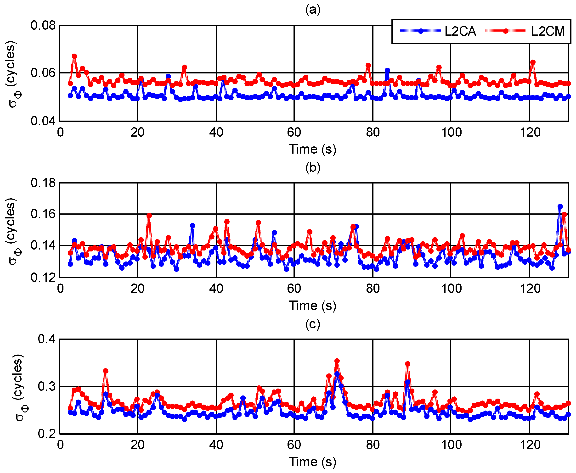
It is noted that the scintillation of carrier phase fluctuation often occurs with less amplitude fading in polar areas, so we focus on the carrier phase fluctuation. In general, $\delta \phi$ > 0.3 cycles indicates strong scintillation with strong carrier phase fluctuation. The $\delta \phi$ indicators for SV #3, 12, and 25 during the simulation are shown in Figure 6.

From Figure 6a we can see that nearly all $\delta \phi$ indices for SV #3 are smaller than 0.1 during the simulation time, which can be considered as weak scintillation. Meanwhile, Figure 6b shows that most of the $\delta \phi$ indices for SV #12 fluctuate between 0.13 and 0.15, which can be regarded as moderate scintillation. Several $\delta \phi$ values approach and even exceed 0.3 for SV #25 in Figure 6c, which represents strong scintillation.

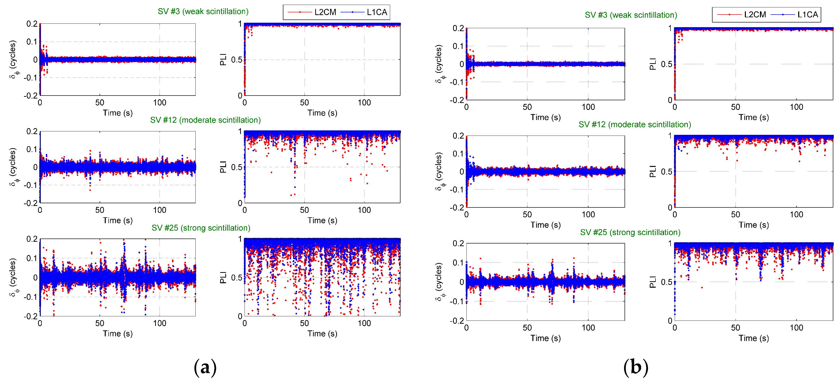
Then, the carrier phase lock indicator (PLI) was used as the criterion of carrier phase tracking performance; it can be expressed as

$$\mathrm{PLI}\approx abs(I_{\mathrm{P}})/\sqrt{\left(I_{\mathrm{P}}^2+Q_{\mathrm{P}}^2\right)}.$$

(34)

The PLI is equal to 1 when the phase is perfectly locked, while it is equal to 0 when the phase lock is lost. In this paper, we use 0.9 and 0.5 as the thresholds of good carrier phase lock and poor carrier phase lock, respectively.

The carrier tracking performances of the three satellite signals using a traditional GNSS tracking loop (a third-order tracking loop with 15 Hz fixed bandwidth, denoted T-GNSS) and the proposed ionosphere-free dual-frequency GNSS/SINS deep-coupled navigation system (denoted IF-DDC) are shown in Figure 7. A summary of the carrier phase tracking performance under scintillation is shown in

Table 5. Summary of tracking performance under scintillation.

Satellite Pseudo Random Noise (PRN) sequences	Method	PLI < 0.9 (Total No. = 11,000)		PLI < 0.5 (Total No. = 11,000)
		L1 CA	L2 CM	L1 CA	L2 CM
SV #3	T-GNSS	0	5	0	0
	IF-DDC	0	2	0	0
SV #12	T-GNSS	112	399	3	12
	IF-DDC	26	119	0	0
SV #25	T-GNSS	950	1766	128	280
	IF-DDC	247	532	0	1

.

It can be seen from Figure 7 and Table 5 that both the T-GNSS and IF-DDC have good carrier phase tracking performance under weak scintillation (i.e., SV #3) during the tracking. The tracking does not have losses during the tracking time. However, the carrier tracking performance of T-GNSS under moderate scintillation (i.e., SV #12) decreases and goes on to suffer large losses under strong scintillation (i.e., SV #25). On the contrary, the carrier tracking of IF-DDC has a much better performance compared with T-GNSS. Although the carrier tracking performance decreases under strong scintillation, most of the PLIs of IF-DDC are still better than 0.5.

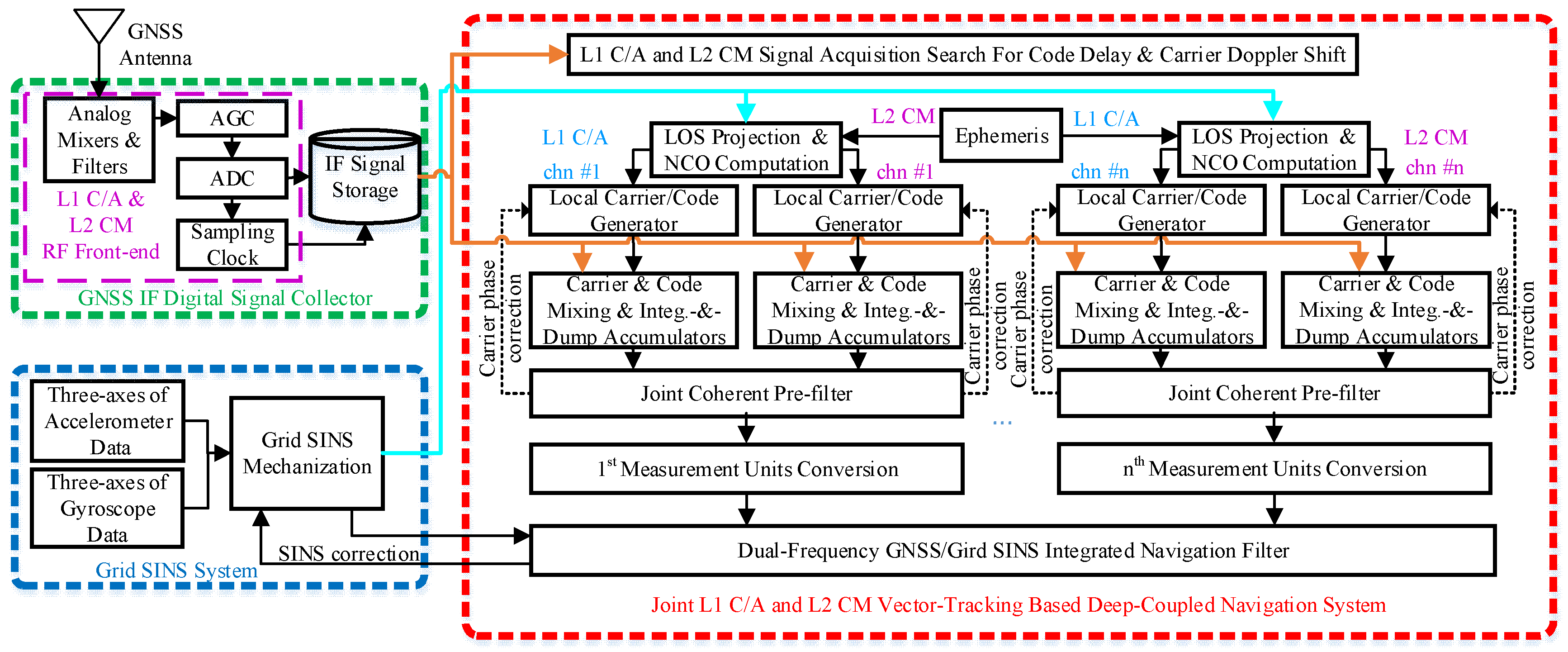
The main reason for the performance improvement of IF-DDC is that the IF-DDC has a joint L1 C/A and L2 CM vector-tracking-based structure, which can provide more measurement information and share better tracking information to aid weak signal channels with strong signal channels. Besides this, the tracking and prefiltering of IF-DDC has adaptive process noise covariance and measurement noise covariance which can reach an optimal equivalent bandwidth during the tracking processing to improve the tracking robustness and accuracy.

It is noted that the L1 C/A signal has a better tracking performance than the L2 CM signal, especially under moderate and strong scintillation, due to the different received RF signal strength and different ionospheric scintillation characters (i.e., ionospheric scintillation strength corresponds to the carrier frequency) between the L1 C/A and L2 CM signals.

4.2.2. Dynamic Test

In the dynamic test, a flight test was set to assess the dynamic performance of the proposed system in polar areas. The parameters of the set of dynamic data are shown in

Table 6. The parameters of the set of dynamic data.

Parameter	Value
Visible satellites	SV # 3	12, 17, 32	1, 6, 25, 31
Maximum C/N0	47 dB-Hz	42 dB-Hz	36 dB-Hz
Ionospheric scintillation interference	Strong (SV #25, 32)
	Moderate (SV #12)
	Weak (SV # 3)
Start point	(85° N, 40° E, 0 m)
Maximum velocity	91 m/s
Maximum acceleration	5 g
Maximum jerk	50 g/s

.

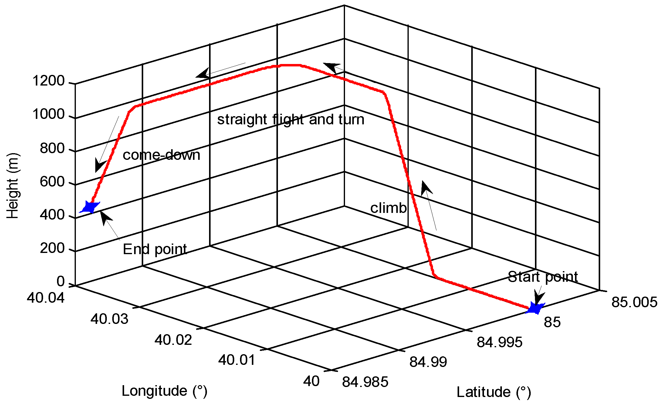
It is noted that the parameters of the visible satellites, C/N₀, and ionospheric scintillation interference in the dynamic test are the same as the parameters in the static test. The flight trajectory for the dynamic test in polar areas is shown in Figure 8.

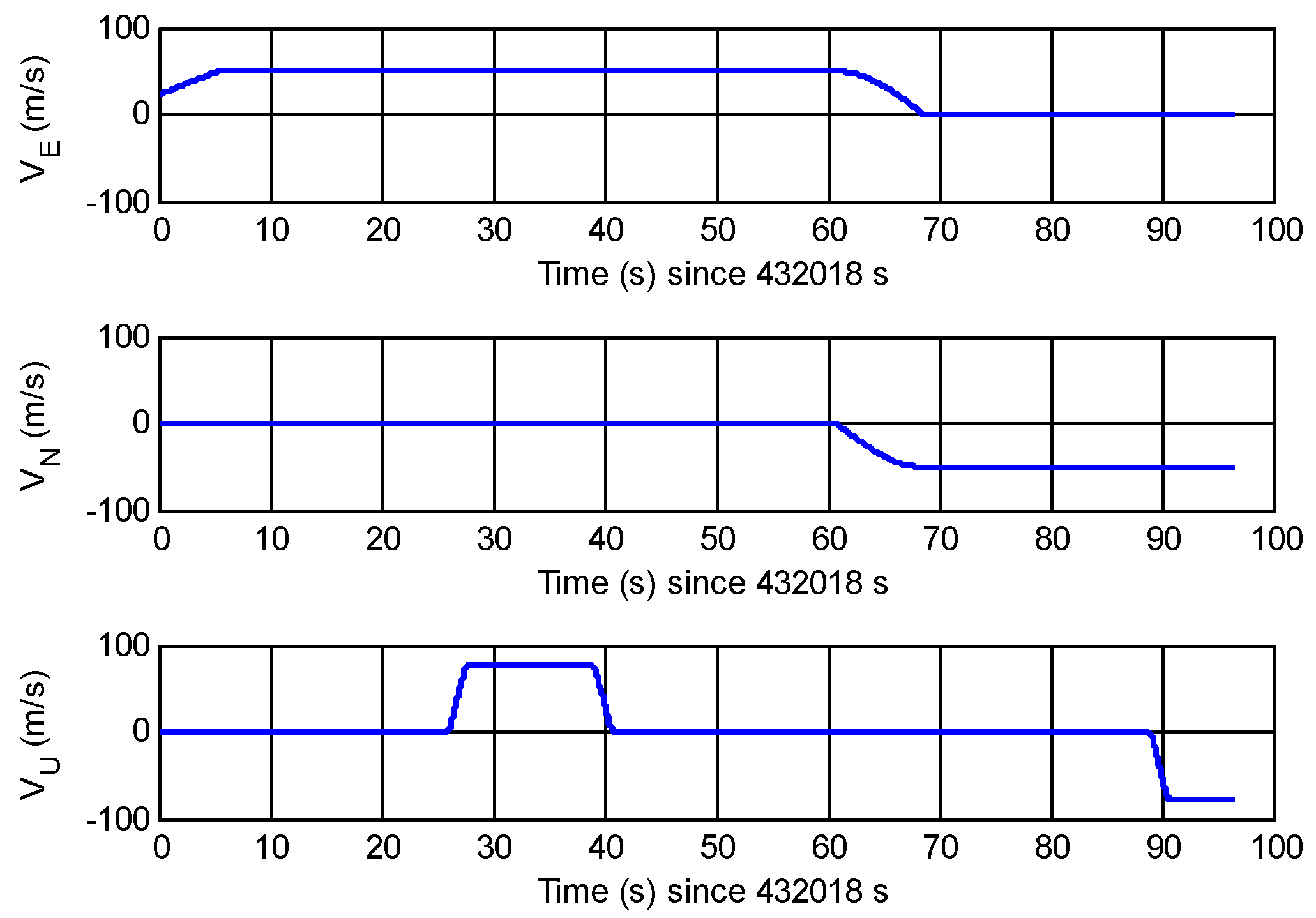
It can be seen that the flight motions include climb, level off, straight flight, turn, and come-down. Meanwhile, the flight velocity and the flight acceleration and jerk are shown in Figure 9 and Figure 10, respectively.

It can be seen that there are several periods of acceleration and jerk with maximum acceleration and jerk of 5g and 50 g/s, respectively. It is noted that the time axis of Figure 9 and Figure 10 starts from 432,018 s which is the start epoch of the system outputting the navigation results after about 34 s of tracking.

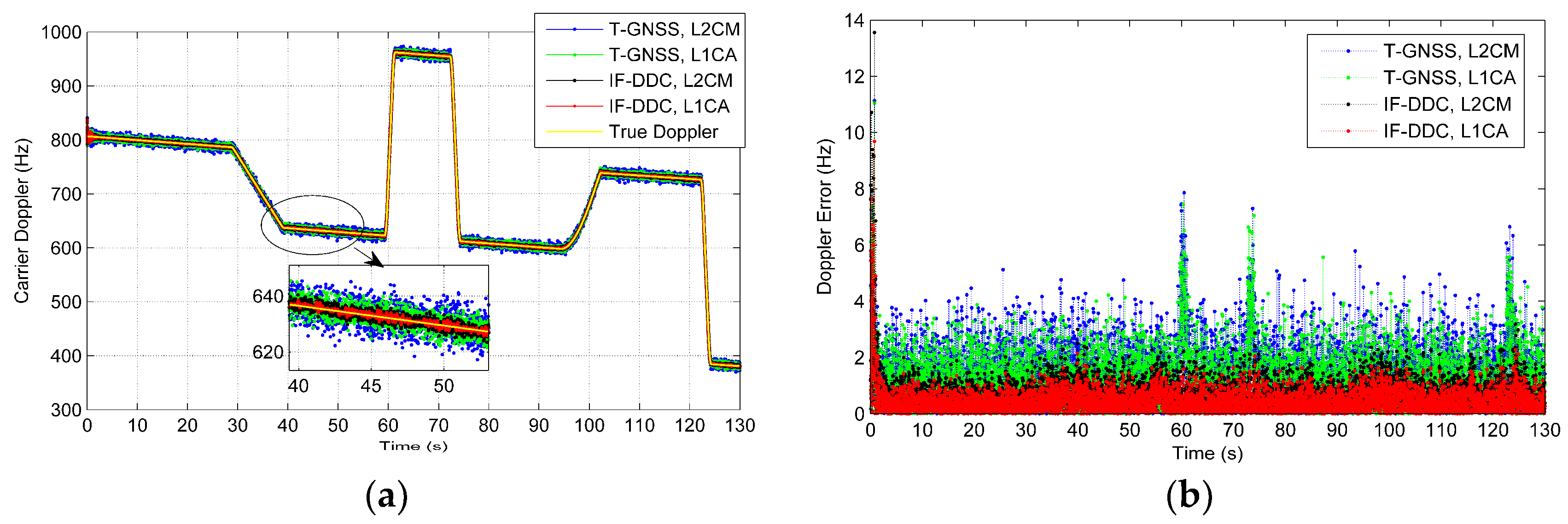
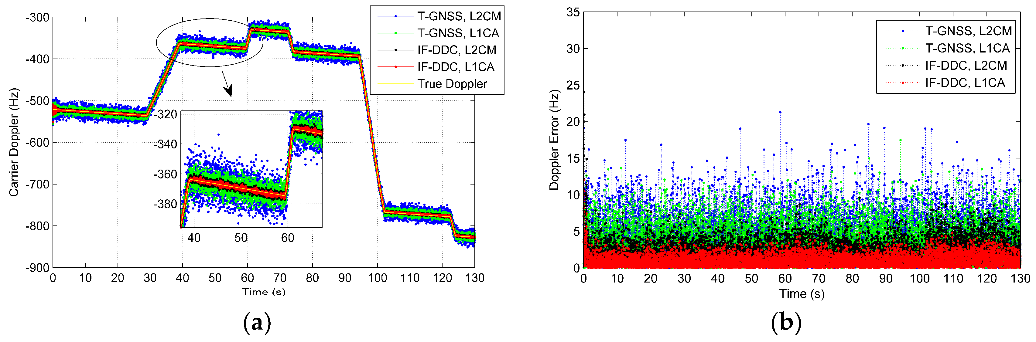
Figure 11 and Figure 12 illustrate the carrier frequency tracking performance using different methods. In this section, the moderate scintillation (i.e., SV #12) and strong scintillation (i.e., SV #25) were focused upon to assess their performance.

It can be seen in Figure 11 that the IF-DDC method allows a reduction in the noise presented in the carrier Doppler compared with the T-GNSS method. The IF-DDC achieves the best performance in terms of noise and scintillation reduction. This is even more evident from Figure 12 where the signal suffers lower C/N₀ and stronger scintillation. Besides this, when compared with Figure 10, some trends related to flight dynamics can be seen in Figure 11b. The transient errors as well as the effects of jerk still remain when the T-GNSS method is used. However, these trends are all removed by the IF-DDC method due to the aid of the grid SINS information.

The results of the tracking performance in the dynamic test show that the proposed IF-DDC method can optimize the tracking band, sharing tracking information to aid the weak signal channels with strong signal channels to reduce the noise and scintillation interference, and utilize SINS information to reduce the dynamic requirement of the tracking loop.

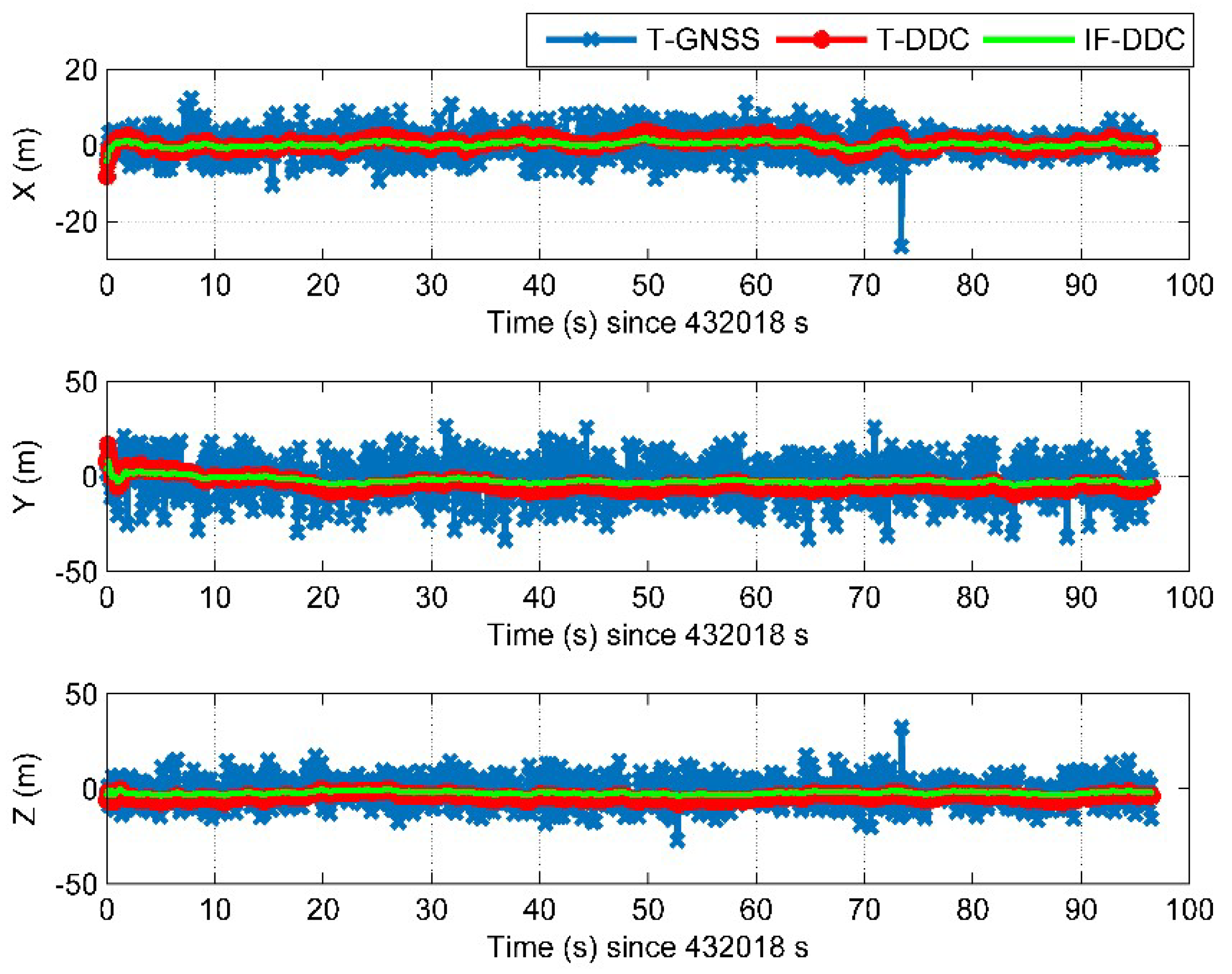
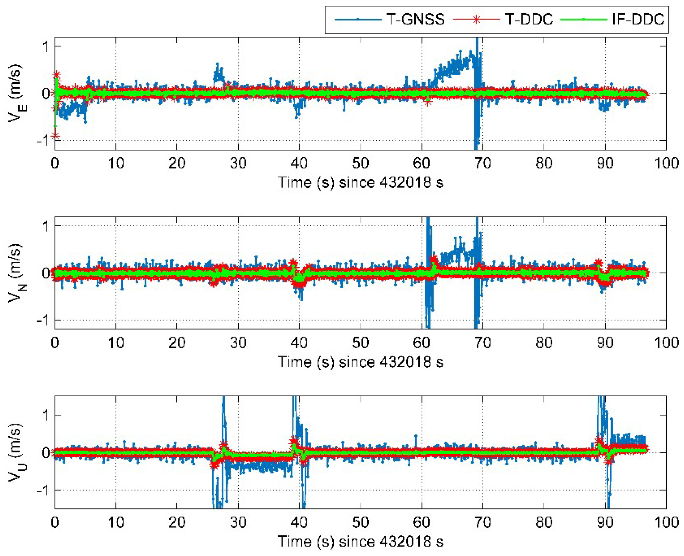
Finally, the position and velocity errors for different methods in the dynamic test are shown in Figure 13 and Figure 14. Similar to Figure 9 and Figure 10, the time axis of Figure 13 and Figure 14 starts from 432,018 s which is the start epoch of the system outputting the navigation results after about 34 s of tracking. In order to assess the effectiveness of the ionosphere-free combination of L1 C/A and L2 CM signals, the non-ionosphere-free dual-frequency deep-coupled navigation (i.e., the L1 C/A and L2 CM signals used as independent information in the system, denoted T-DDC) is also compared in the navigation results.

Table 7. RMS position error statistics of the dynamic test.

Method	RMS Position Errors (m)
	X	Y	Z
T-GNSS	7.0663	10.2338	7.0663
T-DDC	3.6790	2.5797	2.2351
IF-DDC	0.6486	1.2961	1.2655

shows the RMS position error statistics of the dynamic test.

From Figure 13 and Table 7 we can see that both the T-DDC and IF-DDC methods can obtain more accurate position results than the T-GNSS method. Meanwhile, IF-DDC has better position performance than the T-DDC, which indicates that the ionosphere-free combination of L1 C/A and L2 CM signals can further reduce the position error caused by ionospheric delay.

Table 8. RMS velocity error statistics of the dynamic test.

Method	RMS Velocity Errors (m/s)
	VE	VN	VU
T-GNSS	0.261	0.267	0.479
T-DDC	0.049	0.047	0.154
IF-DDC	0.048	0.047	0.153

shows the RMS velocity error statistics of the dynamic test.

As depicted in Figure 14 and Table 8, we also see that both the T-DDC and IF-DDC methods can obtain more accurate velocity results than the T-GNSS method. Moreover, the velocity of T-GNSS is still affected by the effects of jerk, while the velocities of T-DDC and IF-DDC are much smoother than that of T-GNSS during the jerk periods.

As a whole, the proposed IF-DDC method can obtain more stable and accurate navigation performance compared with the traditional T-GNSS method.

5. Conclusions and Future Work

This paper proposes a vector-tracking-based deep-coupled navigation system using dual-frequency GNSS and a grid strapdown inertial navigation system. The hardware simulator and semiphysical experiment results indicate that the proposed system can obtain better navigation accuracy and more stable tracking performance in polar areas compared with the traditional GNSS tracking method. In future work, more realistic experiments will be conducted to further assess the performance of the system, and multiconstellations can be included in the system with the coverage of GNSS satellites increasing in polar areas to further improve the navigation performance.