Article

LIDAR Point Cloud Registration for Sensing and Reconstruction of Unstructured Terrain

1
Department of Mechanical and Electrical Engineering, Xiamen University, Xiamen 361005, China
2
School of Computer Science & Electronic Engineering, University of Essex, Colchester CO4 3SQ, UK
*
Author to whom correspondence should be addressed.
Appl. Sci. 2018, 8(11), 2318; https://doi.org/10.3390/app8112318
Submission received: 21 October 2018 / Revised: 14 November 2018 / Accepted: 18 November 2018 / Published: 21 November 2018
(This article belongs to the Special Issue LiDAR and Time-of-flight Imaging)

Abstract

:
When 3D laser scanning (LIDAR) is used for navigation of autonomous vehicles operated on unstructured terrain, it is necessary to register the acquired point cloud and accurately perform point cloud reconstruction of the terrain in time. This paper proposes a novel registration method to deal with uneven-density and high-noise of unstructured terrain point clouds. It has two steps of operation, namely initial registration and accurate registration. Multisensor data is firstly used for initial registration. An improved Iterative Closest Point (ICP) algorithm is then deployed for accurate registration. This algorithm extracts key points and builds feature descriptors based on the neighborhood normal vector, point cloud density and curvature. An adaptive threshold is introduced to accelerate iterative convergence. Experimental results are given to show that our two-step registration method can effectively solve the uneven-density and high-noise problem in registration of unstructured terrain point clouds, thereby improving the accuracy of terrain point cloud reconstruction.

1. Introduction

In recent years, autonomous navigation technology has been gradually deployed on outdoor vehicles operated in unstructured terrain. Different from structured terrain, unstructured terrain has an uneven surface and complex conditions, which brings a great challenge to the safety and stability of autonomous vehicles. Therefore, various sensors such as visual image sensors [1,2] and LIDAR [3,4] have been deployed on autonomous vehicles for sensing unstructured terrain to achieve safe operation. Although the visual image sensors only produce 2D images, sufficient terrain information can be obtained by using some approaches, such as calculating a height map from an image to obtain 3D information [5] or using the super-resolution reconstruction method to obtain a spatial resolution-enhanced image [6]. Compared with visual image sensors, LIDAR has the advantage of being free from the effect of light and weather and can obtain the three-dimensional terrain information conveniently. Therefore, it has been more and more widely used in autonomous vehicles for navigation purpose.
When LIDAR is used to scan unstructured terrain, the obtained point cloud is uneven in density and noisy due to the influence of the terrain, the land cover [7] and the laser scanning mechanism [8]. Moreover, the point cloud is incomplete because of the self-occlusion of objects and the installing angle of LIDAR. Without sufficient terrain information, the autonomous vehicles will fall into bad performance and even roll over. Therefore, in order to provide sufficient terrain information to autonomous vehicles, it is necessary to register multiple scanning point clouds to obtain an accurate terrain point cloud map. Traditionally, dead reckoning is combined with other sensors for registration [9,10]. Although this method is fast, it can easily lead to a large error in the registration result due to the imprecision of sensor, the sampling difference and the tire slip. Therefore, we propose a new two-step registration method to conduct accurate registration after this initial registration.
The ICP (Iterative Closest Point) algorithm [11] has been widely used for accurate registration; however, it has the disadvantages of low efficiency and of easily falling into local minima. Therefore, many improved ICP algorithms have been proposed to optimize a part of the iterative process and then to improve the traditional ICP algorithm, including nearest point search [12,13,14,15], feature description [16,17], correspondence building [18,19], and convergence judgment [20]. Among them, feature description can effectively conduct the registration of point clouds with uneven-density and high-noise and therefore improve the performance of the traditional ICP algorithm.
In recent years, many scholars have studied the feature description of point cloud. Yao et al. [21] conducted registration by extracting the line and plane features of the point cloud, which can reduce the influence of noise, but requires that the point cloud has obvious line and plane features. Ono et al. [22] and Zhang et al. [23] proposed new feature descriptors with a certain anti-noise ability, but the calculation was complex and time-consuming. Zhang et al. [24] extracted key points based on curvature features without full consideration of the neighborhood of the point, which bring about many feature-similar points when used for the registration of complicated point clouds. The limitations of these methods make them difficult to be used for the fast point cloud reconstruction of unstructured terrains, thus a new feature descriptor is required.
In this paper, we propose a two-step registration method consisting of initial registration and accurate registration. After initial registration, accurate registration is conducted by using an improved ICP based on the neighborhood normal vector, point cloud density and curvature to extract key points and build the new feature descriptor. Compared with the traditional one-step registration method, our method has high accuracy and can reconstruct the point cloud of unstructured terrains quickly. It can effectively solve the accuracy problem of registration for density-uneven and noisy point clouds of unstructured terrains.
The rest of this paper is organized as follows. Section 2 introduces the traditional initial registration method. Section 3 describes our accurate two-step registration method. Four groups of experiments are conducted in Section 4 to validate the feasibility and performance of our two-step registration method. Finally, a brief conclusion and future research directions are given in Section 5.

2. Initial Registration

Figure 1 shows the process of our two-step registration method. By optimizing several key steps shown in yellow, the accuracy and speed for registering field unstructured terrain point clouds are much improved. Specifically, there is an obvious translation and rotation dislocation between the point clouds of consecutive frames when the scanning frequency of LIDAR is low and therefore we firstly use the dead reckoning data to perform initial registration on the point clouds to improve the accuracy and speed of the subsequent accurate registration. In order to implement this method, IMU (Inertial Measurement Unit) is used to obtain attitude data, encoders are used to obtain displacement data, and 3D LIDAR is used to obtain terrain data. These data are matched by using time stamp.
We simplify the calculation by registering the point cloud of the current frame to the navigation coordinate system of the point cloud of the previous frame. The calculation process is as follows:
[ x 0 y 0 z 0 ] = R s ( [ cos α 0 sin α 0 1 0 sin α 0 cos α ] [ x l y l z l ] + [ d l x 0 d l z ] ) + R s [ Δ β r 0 0 ]
where (x0, y0, z0) is the coordinate in the navigation coordinate system of the previous frame; (xl, yl, zl) is the coordinate in the LIDAR coordinate system; α is the angle between the plane of LIDAR and the vertical direction; (dlx, dlz) is the origin of the LIDAR coordinate system relative to the vehicle body coordinate system (IMU coordinate system); Δβ is the encoder increment; r is the tire radius. Rs is as follows:
[ cos θ cos ψ sin ϕ sin θ cos ψ cos ϕ sin ψ cos ϕ sin θ cos ψ + sin ϕ sin ψ cos θ sin ψ sin ϕ sin θ cos ψ + cos ϕ cos ψ cos ϕ sin θ sin ψ sin ϕ cos ψ sin θ sin ϕ cos θ cos ϕ cos θ ]
where (ϕ, θ, ψ) is the vehicle body attitude (Euler angle).
Through formula (2), the point cloud of the current frame is firstly transformed into the vehicle body coordinate system, and then transformed into the current navigation coordinate system, and finally transformed into the previous navigation coordinate system. The point cloud of the previous frame is transformed into its own navigation coordinate system. For subsequent accurate registration, the transformed point cloud of the current frame is the target point cloud and the transformed point cloud of the previous frame is the source point cloud.

3. Accurate Registration

Because of the restriction of the sensor’s precision, there is still a rather big error after the initial registration. Therefore, the accurate registration is necessary to minimize the registration error. Based on the uneven-density and high-noise features in the point clouds of unstructured terrains, an improved ICP algorithm is presented in this section as an accurate registration method.

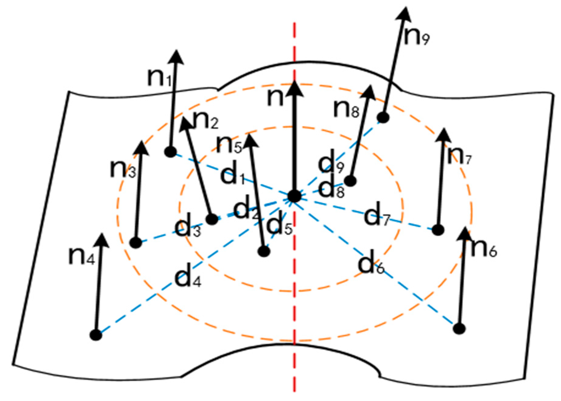
3.1. Key Points Extraction

In the original point cloud, there are some representative points with rich feature information. Extracting these points to form a key point set can improve registration accuracy and speed. Jiang et al. [25] used the mean angle between the normal vectors of one point and its k-nearest neighbor points as the angle-invariant feature, which has strong sensitivity to the local surface change, but do not consider the spatial distribution of these neighbor points. Therefore, the feature cannot correctly reflect the surface change in a local area where the points are sparse.
As shown in Figure 2, when a different number of neighbor points is taken to calculate angle-invariant features of point in uneven area, there is a big difference in the result. This is because the more neighborhood points are taken, the more points in the flat area will be included into calculation. This will significantly influence the evaluation of convexity degree of area around the point.
Therefore, we introduce neighborhood weighting to optimize the algorithm. The improved algorithm is used to extract key points with rich feature information from the point cloud of unstructured terrains. The key points are extracted as follows:
f i = j = 1 k d i j m j = 1 m ( n i n j | n i | | n j | 1 d i j )
where fi is the neighborhood weighted angle-invariant feature, ni and nj are the normal vectors of point, dij is the spatial distance between the point and the neighbor point, m is the number of neighbor points.
We set an appropriate threshold ε here. If fi > ε, it means the local surface change of the point is small and the point should be discarded; if fi < ε, it means the local surface change of the point is large and the point should be kept as a key point. Through this way, we can obtain the key point sets of source point clouds and target point clouds.

3.2. Building Neighborhood Feature Descriptor

We built the corresponding relation between the two key point sets by finding similar feature points. The point feature descriptor directly affects the iteration speed and registration accuracy. We propose a seven-dimensional neighbourhood feature descriptor. First of all, the curvature has the invariance of rotation, translation, and scaling, so it is considered as a feature element. The curvature k is calculated as follow [26]:
k = λ 0 λ 0 + λ 1 + λ 2
where λ is from formula:
C v i = λ i v i , i { 0 , 1 , 2 }
where C is the covariance matrix of point, v is the eigenvector and λ is the eigenvalue.
Then taking into account the spatial distribution and feature of the neighbor points, we add two feature elements u and v:
u i = 1 m j = 1 m d i j k j ,      v i = 1 m j = 1 m d i j f j
where dij is the spatial distance from one point to its neighbor point, kj is the curvature of the neighbor point, fj is the neighborhood weighted angle-invariant feature, m is the number of neighbor points.
It should be noticed that x, y, z, f, k, u, and v constitute our feature descriptor, in which x, y, z are the coordinates of point, f is the neighborhood weighted angle-invariant feature, k is the curvature, u and v are from formula (6). We use the data obtained by calculating the normal vectors of points to build a feature that fully expresses the neighborhood information, thus the speed and accuracy of feature calculation and correspondence building are improved.

3.3. Transform Matrix Calculation

In each iteration, a threshold is required when building links between points with the help of features. If the Euclidean distance between two points is less than the threshold, the link between the two points will be preserved. We propose to set the adaptive threshold to speed up the iteration. The threshold is reduced after each iteration. The RANSAC algorithm is used to further remove incorrect links. In the process of finding the optimal transformation through the corresponding relation, we use the algorithm proposed by Low [27] to find the transformation matrix. When θ ≈ 0, there is sinθ ≈ 0, cosθ ≈ 1. According to this, when α, β, γ ≈ 0, we have:
M = T ( t x , t y , t z ) R ( α , β , γ ) T ( t x , t y , t z ) R ^ ( α , β , γ ) = M ^
where T is the transformation matrix, R is the rotation matrix, R ^ is the approximate rotation matrix, M is the 3D rigid transformation matrix and M ^ is the approximate 3D rigid transformation matrix.
After the above approximation, the original nonlinear problem is converted into a linear problem. The linear least-squares method can then be used to calculate the optimal transformation matrix by using the following equation:
M o p t = arg min M ^ i ( ( M ^ s i d i ) n i ) 2
where Mopt and M ^ are the 4 × 4 transformation matrixes, Si is the source point, di is the target point, and ni is the normal vector of the target point.

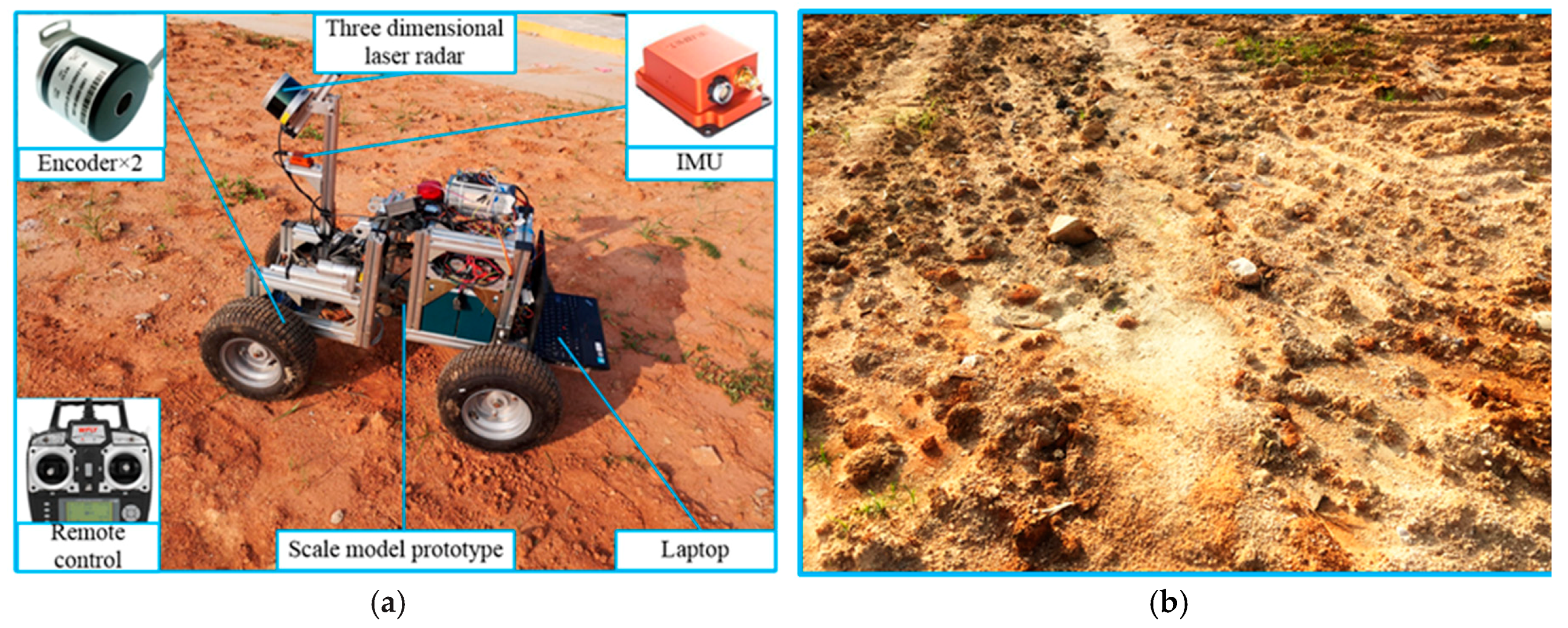
4. Experimental Results and Analysis

Figure 3a shows the mobile platform used in the experiments, in which multiple sensors and other components are highlighted. More specifically, three types of sensors, IMU, LIDAR (laser scanner), 2 incremental encoders, are used for scanning and registration of terrain point cloud. Detailed information about these sensors is shown in Table 1. The articulated wheel loader has 4 wheels and a joint connection of front and back bodies. A laptop PC and a remote controller are used to control its motion and collect data. Figure 3b is a typical unstructured terrain. This terrain has strong unstructured feature, and we use its scanned point clouds to do the following registration experiment.

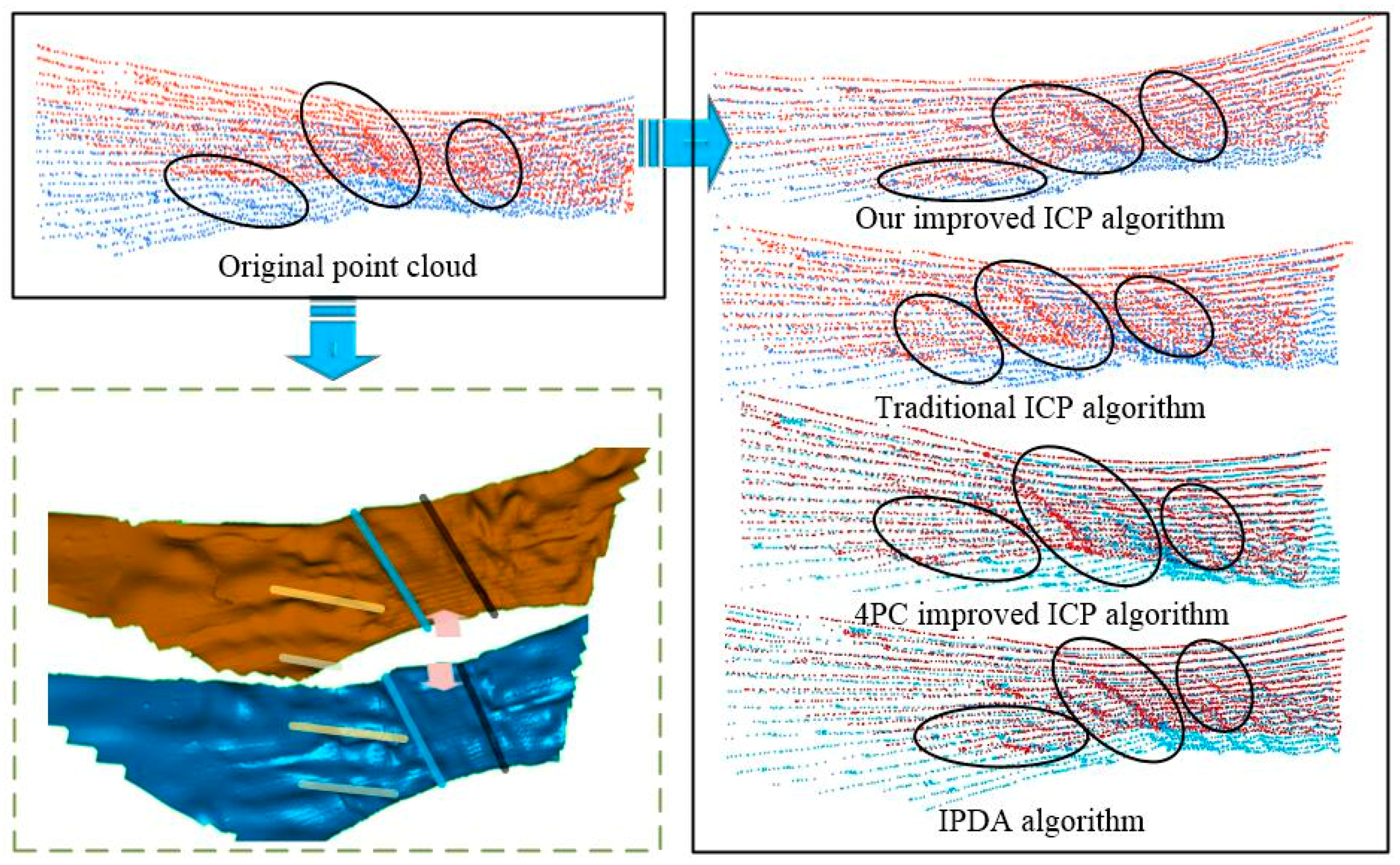
4.1. Validity Validation of our Improved ICP Algorithm

To verify the performance of our improved ICP algorithm, the point clouds of two consecutive frames of unstructured terrain shown in Figure 3b are used for registration experiments. Figure 4 shows the registration process. More specifically, Figure 4a is the point cloud after initial registration and filtering. Since the two point clouds still have a certain dislocation, the local features in the point cloud are not obvious. Figure 4b shows the key point extraction result of Figure 4a. It can be seen that the key points are concentrated in the area where the neighborhood undulates greatly. This clearly shows that our key point extraction method not only greatly reduces the number of points but also fully preserves the local features of unstructured terrain point cloud.
Figure 4c shows the links between the key points. Due to the existence of feature-similar points, there is a case where one point is linked to multiple points. However, as all the linked lines are parallel to each other, this proves that the overall accuracy of the linked point search is high. Figure 4d shows the results of the registration. Compared with Figure 4a, the gully feature is obvious, and the bulges and pits are aligned, which verifies the good performance of our ICP algorithm.

4.2. Superiority Validation of our Improved ICP Algorithm

To verify the superiority of our improved ICP algorithm for the point cloud registration of unstructured terrains, we take two point cloud pairs to conduct contrast experiments. Our experiment process is described below:
(1)
Conduct initial registration and filtering for the original point cloud pair to obtain the source point cloud and the target point cloud.
(2)
Use our improved ICP algorithm to register target point cloud with source point cloud, and then record the data.
(3)
Use our key point extraction method to obtain the key point sets of the source point cloud and the target point cloud, and then use traditional ICP algorithm, 4PC improved ICP algorithm [28] and IPDA (Integrated Probabilistic Data Association) algorithm [29] separately to register the two key point sets, and finally record the data.
We take the points in source point cloud as the object to find the nearest neighbor point in the target point cloud. When the point-to-point distance exceeds a certain threshold, these two points will be regarded as the points outside the overlap area and then be abandoned, the root mean square error (RMSE) of the remaining point-to-point distances is calculated as the evaluation standard of registration accuracy. The result is shown in Table 2. Compared with the traditional ICP algorithm and 4PC improved ICP algorithm, the single iteration time of our algorithm is greatly reduced, and the error is smaller. This is because the traditional ICP algorithm is based on the nearest distance to find the link points, it is not suitable for density-uneven and high-noise field unstructured terrain point cloud. The 4PC improved ICP algorithm replaces the original greedy search strategy by using a 4-points consistent point search strategy. Although it can improve the efficiency of traditional ICP algorithm and deal with the noise in point cloud, its ability is restricted. The IPDA algorithm improves standard ICP data association policy by using Probabilistic Data Association. Compared with the IPDA algorithm, the registration speed of our improved ICP algorithm is much faster, but slightly less accurate in registration. Because of the special data association and weight calculation, the IPDA algorithm is so time-consuming and not suitable for fast reconstruction.
Figure 5 shows the registration result of PCPair2 (point cloud pair) using different algorithms. The 3D graph is the 3D reconstruction of source point cloud and target point cloud. As shown in this 3D graph, there are four distinct gullies. After the accurate registration using our improved ICP algorithm and IPDA algorithm, the four gullies in the two point clouds have been aligned and the features of result point cloud are obvious. In contrast, when using the traditional ICP algorithm and 4PC improved ICP algorithm to register, the gullies have obvious misalignment due to the registration error.

4.3. Necessity Validation of the Initial Registration

To verify the validity and necessity of the initial registration, we take three point cloud pairs of the unstructured terrain (Figure 3b) to conduct experiments. Each point cloud pair consists of two point clouds of consecutive frames. The experiments register three point cloud pairs in two cases: (i) initial registration and accurate registration; (ii) accurate registration only.
The experimental results are shown in Table 3. As can be seen, the iteration number and registration time increase significantly without initial registration, and the registration error also increases relatively. Figure 6 shows the results of registration with and without initial registration. More specifically, Figure 6a shows the original point cloud. Figure 6b shows the point cloud after initial registration. Figure 6c shows the point cloud after accurate registration. Figure 6d shows the point cloud by using our two-step registration method, i.e., initial registration and accurate registration. It is clear that this results in higher accuracy than the single-step registration approach.

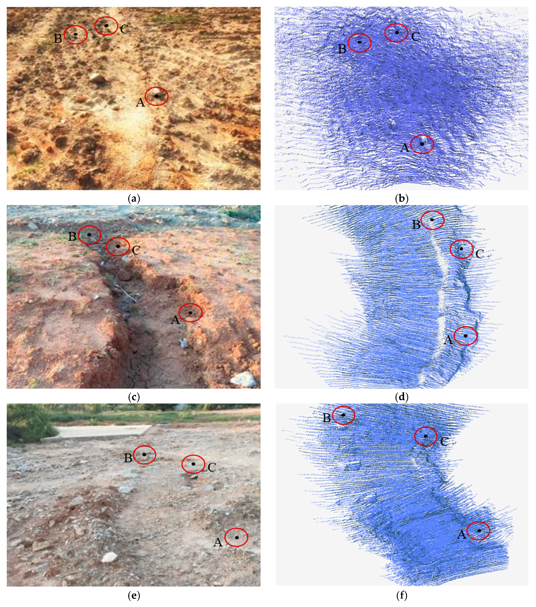
4.4. Fast Acquisition of Point Cloud Information for Timeliness Demand

To verify the feasibility in the real-world application, we conducted experiments using our built-in-house mobile platform to perform the continuous scanning and registration of point clouds for unstructured terrains. After acquiring the terrain point cloud of the current frame, the system performs the initial registration and accurate registration on it with the terrain point cloud of the previous frame, and then transforms it into the global coordinate system. Table 4 presents the program implementation of this process. In the experiment, the speed of our mobile platform is set to 0.5 m/s, the acquisition frequencies of terrain point cloud, IMU data, and encoder data are set to 1 Hz, 100 Hz, and 100 Hz, respectively.
To fully verify the validity and universality of our method for unstructured terrains, we chose three types of unstructured terrains as the experiment sites, as shown in Figure 7. More specifically, Figure 7a shows an unstructured terrain with small gullies and stones; Figure 7c shows an unstructured terrain with deep pits and stones; and Figure 7e shows an unstructured terrain with big bulges and stones. The experiment results are shown in Figure 7b,d,f. The characteristics of the actual terrain are well expressed by the terrain point cloud being generated, such as ditch, ridge, pit, bulge, and stone.
To further verify the quality of registration, we take three points A, B, and C that are easy to distinguish as shown in Figure 7. Firstly, we measure the distance from A to B in the actual terrain and terrain point cloud, denoted as dAB and d AB respectively. Then, we measure the distance from A to C in the actual terrain and terrain point cloud, denoted as dAC and d AC , respectively. Finally, we calculate τ = d AB d AC / d AC d AB .
Table 5 presents the details of measurement and calculation of deformation. The deviation between the measured value in the point cloud and the actual value is in the millimeter range and τ is close to 1. These show that the translation and rotation deformation of terrain point clouds is small, and it can provide accurate information of the actual unstructured terrain. Therefore, our two-step registration method can be applied to the fast point cloud reconstruction of various unstructured terrains and is fast enough so that the information can be acquired quickly.

5. Conclusions

This paper proposes a two-step registration method for fast point cloud reconstruction of unstructured terrains. Our method firstly uses multi-sensor data and dead reckoning for initial registration. The improved ICP algorithm is then used to perform accurate registration. There are two major contributions made in this paper. One is a simple and effective key point extraction and feature description method deployed for accurate registration, and another is the introduction of adaptive threshold to accelerate iterative convergence. Experimental results show that our two-step registration method is simple and effective, and can be applied to the timely acquisition of unstructured terrain information.
In general, continuous registrations bring cumulative errors, which could ultimately affect the accuracy of the acquired unstructured terrain point cloud. In the future work, we will consider introducing a suitable graph optimization method to reduce the cumulative error and ensure the timely implementation.

Author Contributions

Q.Z. and H.H. conceived and designed the experiments, wrote the paper; J.W. and C.X. performed the experiments and analyzed the data; W.C. helped revise the paper.

Funding

This work was financially supported by the National Natural Science Foundation of China (Grant No. 51575463), as well as the Fujian Collaboration Innovation Center for R&D of Coach and Special Vehicle (Grant No. 2016BJC016), Key Technology R&D Program of Fujian (2016HZ0001-9) and was supported by the scholarship under the education department of Fujian province.

Conflicts of Interest

The authors declare no conflict of interest.

References

  1. Oskiper, T.; Sizintsev, M.; Branzoi, V.; Samarasekera, S.; Kumar, R. Augmented Reality binoculars. IEEE Trans. Vis. Comput. Gr. 2015, 21, 611–623. [Google Scholar] [CrossRef] [PubMed]
  2. Lv, Z.Y.; Shi, W.Z.; Zhou, X.C.; Benediktsson, J. Semi-Automatic System for Land Cover Change Detection Using Bi-Temporal Remote Sensing Images. Remote Sens. 2017, 9, 1112. [Google Scholar] [CrossRef]
  3. Han, M.; Bo, Z.; Qian, K.; Fang, F. 3dlocalization and mapping of outdoor mobile robots using a Lidar. J. Huazhong Univ. Sci. Technol. 2015, 43, 315–318. [Google Scholar]
  4. Gézero, L.; Antunes, C. An efficient method to create digital terrain models from point clouds collected by mobile lidar systems. ISPRS Int. Arch. Photogramm. Remote Sens. Spati. Inf. Sci. 2017, 42, 289–296. [Google Scholar] [CrossRef]
  5. Van der Mark, W.; Groen, F.C.A.; Van Den Heuvel, J.C. Stereo based navigation in unstructured environments. In Proceedings of the IEEE Conference on Instrumentation and Measurement Technology, Budapest, Hungary, 21–23 May 2001; Volume 3, pp. 2038–2043. [Google Scholar]
  6. Zhang, T.; Du, Y.; Lu, F. Super-Resolution Reconstruction of Remote Sensing Images Using Multiple-Point Statistics and Isometric Mapping. Remote Sens. 2017, 9, 724. [Google Scholar] [CrossRef]
  7. Balsa-Barreiro, J.; Lerma, J.L. Empirical study of variation in Lidar point density over different land covers. Int. J. Remote Sens. 2014, 35, 3372–3383. [Google Scholar] [CrossRef]
  8. Balsa-Barreiro, J.; Avariento, J.P.; Lerma, J.L. Airborne light detection and ranging (Lidar) point density analysis. Sci. Res. Essays 2012, 7, 3010–3019. [Google Scholar] [CrossRef]
  9. Li, R.; Liu, J.; Zhang, L.; Hang, Y. LIDAR/MEMS IMU integrated navigation (SLAM) method for a small UAV in indoor environments. In Proceedings of the Inertial Sensors and Systems Symposium, Karlsruhe, Germany, 16–17 September 2014; pp. 1–15. [Google Scholar]
  10. Zhang, X.; Shi, H.; Pan, J.; Zhang, C. Integrated navigation method based on inertial navigation system and Lidar. Opt. Eng. 2016, 55, 044102. [Google Scholar] [CrossRef]
  11. Besl, P.; Mckay, N. A method for registration for 3D shapes. In Sensor Fusion IV: Control Paradigms and Data Structures; International Society for Optics and Photonics: San Diego, CA, USA, 1992. [Google Scholar]
  12. Li, W.; Song, P. A modified ICP algorithm based on dynamic adjustment factor for registration of point cloud and CAD model. Pattern Recognit. Lett. 2015, 65, 88–94. [Google Scholar] [CrossRef]
  13. Li, S.; Wang, J.; Liang, Z.; Su, L. Tree point clouds registration using an improved ICP algorithm based on kd-tree. In Proceedings of the Geoscience and Remote Sensing Symposium, Beijing, China, 10–15 July 2016; pp. 4545–4548. [Google Scholar]
  14. Liu, J.; Zhang, X.; Zhu, J. ICP three-dimensional point cloud registration based on K-D tree optimization. Eng. Surv. Map. 2016, 25, 15–18. [Google Scholar]
  15. Wang, K.; Li, X.; Lei, H.; Zhang, X. An ICP algorithm based on block path closest point search. In Journal of Physics Conference Series; IOP Publishing: Bristol, UK, 2017; p. 012063. [Google Scholar]
  16. Zheng, Z.; Li, Y.; Wang, J. LiDAR point cloud registration based on improved ICP method and SIFT feature. In Proceedings of the IEEE International Conference on Progress in Informatics and Computing, Nanjing, China, 18–20 December 2016; pp. 588–592. [Google Scholar]
  17. Yang, B.; Zang, Y. Automated registration of dense terrestrial laser-scanning point clouds using curves. ISPRS J. Photogramm. Remote Sens. 2014, 95, 109–121. [Google Scholar] [CrossRef]
  18. Ye, Q.; Yao, Y.; Gui, P.; Lin, Y. An improved ICP algorithm for Kinect point cloud registration. In Proceedings of the International Conference on Natural Computation, Fuzzy Systems and Knowledge Discovery, Changsha, China, 13–15 August 2016; pp. 2109–2114. [Google Scholar]
  19. Hou, D.X.; Wang, Y.H.; Zong-Chun, L.I. Constraints improved ICP algorithm based on eliminating error correspondence points. Sci. Surv. Mapp. 2015, 40, 103–107. [Google Scholar]
  20. Mitra, N.J.; Gelfand, N.; Pottmann, H.; Guibas, L. Registration of point cloud data from a geometric optimization perspective. In Proceedings of the 2004 Eurographics/ACM SIGGRAPH symposium on Geometry processing, Nice, France, 8–10 July 2004; pp. 22–31. [Google Scholar]
  21. Yao, J.; Ruggeri, M.R.; Taddei, P.; Sequeira, V. Automatic scan registration using 3D linear and planar features. 3D Res. 2010, 1, 22. [Google Scholar] [CrossRef]
  22. Ono, K.; Ono, R.; Hanada, Y. 3D surface registration using estimated local shape variation. In Proceedings of the IEEE Conference on Control Technology and Applications, Kohala, HI, USA, 27–30 August 2017; pp. 1362–1367. [Google Scholar]
  23. Zhang, X.Ð.H.; Gao, X.J. Registration of Point Clouds Based on Differential Geometry of Surfaceâ™s Feature. Appl. Mech. Mater. 2011, 101–102, 232–235. [Google Scholar]
  24. Zhang, X.J.; Zhong-Ke, L.I.; Wang, X.Z.; Pei-Jun, L.; Wang, Y. Research of 3D point cloud data registration algorithms based on feature points and improved ICP. Trans. Microsyst. Technol. 2012, 31, 116–248. [Google Scholar]
  25. Jiang, J.; Cheng, J.; Chen, X. Registration for 3-D point cloud using angular-invariant feature. Neurocomputing 2009, 72, 3839–3844. [Google Scholar] [CrossRef]
  26. Rusu, R.B. Semantic 3D Object Maps for Everyday Manipulation in Human Living Environments. KI Künstliche Intelligenz 2010, 24, 345–348. [Google Scholar] [CrossRef] [Green Version]
  27. Low, K.L. Linear Least-Squares Optimization for Point-To-Plane ICP Surface Registration; University of North Carolina: Chapel Hill, NC, USA, 2004. [Google Scholar]
  28. Liu, J.; Shang, X.; Yang, S.; Shen, Z. Research on Optimization of Point Cloud Registration ICP Algorithm. In Proceedings of the Pacific-Rim Symposium on Image and Video Technology, Sydney, Australia, 18–22 November 2017; pp. 81–90. [Google Scholar]
  29. Agamennoni, G.; Fontana, S.; Siegwart, R.Y.; Sorrenti, D.G. Point Clouds Registration with Probabilistic Data Association. In Proceedings of the IEEE International Conference on Intelligent Robots and Systems, Daejeon, Korea, 9–14 October 2016; pp. 4092–4098. [Google Scholar]
Figure 1. The process of our two-step registration method.
Applsci 08 02318 g001
Figure 2. The influence of neighbor points for the calculation of the angle-invariant feature.
Applsci 08 02318 g002
Figure 3. System hardware and main experiment object. (a) System hardware; (b) Main experiment object. IMU: Inertial Measurement Unit.
Applsci 08 02318 g003
Figure 4. Registration process of our improved ICP algorithm. (a) Original point cloud; (b) Key point extraction; (c) Links between features; (d) Point cloud after registration. ICP: Iterative Closest Point.
Applsci 08 02318 g004
Figure 5. Comparison of different registration algorithms for PCPair2. IPDA: Integrated Probabilistic Data Association; PCP: point cloud pair.
Applsci 08 02318 g005
Figure 6. Result of registration with and without initial registration for PCPair3. (a) Original point cloud; (b) Point cloud after initial registration; (c) Point cloud after accurate registration; (d) Point cloud after initial and accurate registration.
Applsci 08 02318 g006
Figure 7. Results of field unstructured terrain point cloud reconstruction. (a) Small gully terrain; (b) Small gully terrain point cloud; (c) Deep pit terrain; (d) Deep pit terrain point cloud; (e) Big bulge terrain; (f) Big bulge terrain point cloud.
Applsci 08 02318 g007
Table 1. Information of Main Sensors.
EquipmentSpecifications
Laser scanner (vlp-16)Measurement range: up to 100 m, Accuracy: ±3 cm (typical), Angular resolution(horizontal): 0.1–0.4°, 100 × 65 mm, 0.83 kg
IMU (Xsens MTi-700)Latency: <2 ms, Gyroscopes: 450°/s, Accelerometers: 200 m/s2, 57 × 42 × 23 mm, 0.055 kg
Encoder (E6B2-CWZ6C)Incremental, Resolution: 1000 P/R, Maximum speed: 6000 r/min, φ40 mm, 0.085 kg
Table 2. Result Comparison of Different Registration Algorithms.
Point Cloud Pair (Point Number)AlgorithmKey Point NumberIteration NumberAverage Registration Time/msRegistration Error/m
PCPair1 (17456,17728)Our improved ICP677,56186320.004456
Traditional ICP677,561712260.009770
4PC improved ICP677,56169560.008124
IPDA677,561851200.004221
PCPair2 (17920,17856)Our improved ICP580,576127620.003982
Traditional ICP580,5761514900.004877
4PC improved ICP580,5761311620.004543
IPDA580,5761262350.003542
Table 3. Result of Registration with and without Initial Registration.
Point Cloud PairWithout Initial RegistrationWith Initial Registration
Iteration NumberAverage Registration Time/msRegistration Error/mIteration NumberAverage Registration Time/msRegistration Error/m
PCPair11310430.00695486320.004456
PCPair21410300.004543127620.003982
PCPair3129600.004643116960.004572
Table 4. Pseudo Code of Fast Registration of Point Clouds.
Algorithm 1 Align Point Clouds (C, L, P, D).
Input: Point cloud of current frame C, point cloud of previous frame L, IMU data set P, encoder data set C
Output: Point cloud of current frame that transformed to the global coordinate
⊳Initial registration
for eachp1P do
ifL.timestamp = p1.timestamp then ⊳Find corresponding attitude data by time stamp
  return p1
end if
end for
for eachd1D do
ifL.timestamp = d1.timestamp then ⊳Find corresponding displacement data by time stamp
  return d1
end if
end for
transformCloud(L, p1, 0) ⊳Function: transform the point cloud of previous frame into its own navigation coordinate system
for eachp2P do
ifC.timestamp = p2.timestamp then ⊳Find corresponding attitude data by time stamp
  return p2
end if
end for
for eachd2D do
ifC.timestamp = d2.timestamp then ⊳Find corresponding displacement data by time stamp
  return d2
end if
end for
transformCloud(C, p2, d2d1) ⊳Function: transform the point cloud of current frame to the navigation coordinate system of previous frame
⊳Accurate registration
pairTransform ← pairAlign(L, C) ⊳Function: accurate registration, return the matrix
⊳Transform the point cloud to the global coordinate system which is the navigation coordinate system of the first input point cloud
transformPointCloud(C, globalTransformpairTransform)
⊳Calculate the transformation from C1 to C2, C1 is the point cloud obtained by transforming C into its own navigation coordinate system, C2 is the point cloud obtained by transforming c into the navigation coordinate system of previous frame.
transform_ ← computeTransform(p2, d2d1)
⊳Update global transformation
globalTransformglobalTransformpairTransformtransform_
returnC
Table 5. Measurement and Calculation of Deformation.
Unstructured TerrainActual Terrain/mTerrain Point Cloud/m τ = d AB d AC d AC d AB
d A B d A C d A B d A C
Small gully terrain2.592.612.52222.53100.9958
Deep pit terrain2.622.032.59231.99090.9912
Big bulge terrain4.012.873.96222.82810.9972

