Microparticle Manipulation and Imaging through a Self-Calibrated Liquid Crystal on Silicon Display

Abstract

We present in this paper a revision of three different methods we conceived in the framework of liquid crystal on silicon (LCoS) display optimization and application. We preliminarily demonstrate an LCoS self-calibration technique, from which we can perform a complete LCoS characterization. In particular, two important characteristics of LCoS displays are retrieved by using self-addressed digital holograms. On the one hand, we determine its phase-voltage curve by using the interference pattern generated by a digital two-sectorial split-lens configuration. On the other hand, the LCoS surface profile is also determined by using a self-addressed dynamic micro-lens array pattern. Second, the implementation of microparticle manipulation through optical traps created by an LCoS display is demonstrated. Finally, an LCoS display based inline (IL) holographic imaging system is described. By using the LCoS display to implement a double-sideband filter configuration, this inline architecture demonstrates the advantage of obtaining dynamic holographic imaging of microparticles independently of their spatial positions by avoiding the non-desired conjugate images.

1. Introduction

The interest of using Liquid Crystal on Silicon (LCoS) displays to implement wavefront modulation has been widely discussed in literature [1,2,3,4]. LCoS displays are reflective Liquid Crystal Displays (LCDs) that can be customized to operate as spatial light modulators (SLMs). Into the LCoS architecture, LC molecules are evenly distributed on a thin layer with a pixelated aluminum array connected beneath. Underneath the aluminum pixel array, an electronic circuity is integrated into the silicon chip, which allows controlling the voltages addressed to any pixel in the display [3]. Once the voltage is driven to the LC molecules in each pixel, they tend to align with the applied electric field. Importantly, LC molecules orientation varies with the applied voltage, and thus, different phase retardation is introduced as a function of the voltage. When the system is optimized to work into the phase-only regime (by controlling the polarization of light illuminating the display [5]), the wavefront phase distribution can be spatially modified by addressing the proper voltage-inspired phase retardation distribution.

Note that LCoS displays can be configured to both operating in the amplitude-only or the phase-only regimes. Into the amplitude modulation scheme, output intensity distribution can be customized by properly modifying the polarization spatial distribution of the wavefront, and projecting it over a linear analyzer, being this configuration commonly used for imaging proposes. Conversely, LCoS displays operating in the phase-only regime are commonly used for phase modulation, being of interest in a wide number of applications, such as microstructure fabrication [6], holography [7,8], biomedical applications [9], waveguide optics [10], optical switching [11], microparticle manipulation [12,13], etc. To guarantee an optimal working performance in all those applications, LCoS must be previously calibrated and optimized. In particular, the phase-voltage relation and the LCoS surface homogeneity (flatness) are two important characteristics to be calibrated as they directly determine the performance of the generated phase distribution [14,15,16]. In this paper, we review a novel method able to provide both characteristics in a compact and feasible optical arrangement. The method is based on the use of diffractive optical elements (DOEs) self-addressed to the LCoS display to be optimized. Here, the term “self-addressing” means that the used DOEs are addressed to the same LCoS display to be calibrated, this leading to an auto-calibrating procedure. In particular, two DOEs are self-addressed: (1) a split-lens configuration [17,18] to fulfil the phase-voltage calibration; and (2) a spot-array pattern (Shack–Hartmann, S-H, configuration [19,20,21]) to realize the surface profile measurement. For the phase-voltage calibration case, a diffractive two split-lens configuration is addressed on the LCoS, which is illuminated by coherent light. This configuration is equivalent to the Young’s double slit experiment, so the well-known fringes pattern is realized to a propagated plane. Later, by adding different constant phases (by driving different voltages) to one of the two split-lenses phase distributions, the fringes pattern is shifted in the transversal direction according to the added phase. Under this scenario, the LCoS phase-voltage relation is directly obtained by analyzing the interferometry pattern shift within each driven voltage. Here, we want to note that our interferometry-based technique demonstrates great advantage compared to other existing schemes. For instance, the method is able to take into account the unsatisfied time-fluctuation effect (also refereed as flicker effect [22]) that degrades the performance of LCoS, without requiring extra metrological set-ups (i.e., the system is self-calibrated). For the surface profile calibration case, a highly collimated beam illuminates the LCoS display where an S-H configuration has been implemented. After reflection on the LCoS display, the input light creates a spot array distribution at the micro-lens focal plane. If the input light is highly collimated, light dots deviations from a reference dots-pattern are mainly originated by inhomogeneity at the LCoS screen. At this moment, by calculating the deviation of each individual spot to its theoretical center, the surface profile can be accurately retrieved by using numerical methods.

Once the LCoS display is optimized, we use it for optical applications. Two different applications we recently developed for microparticles imaging [23,24] and manipulation [12,13] are revised in this manuscript. First, we use such elements to realize customized three-dimensional light structures. Due to photophoretic force fields [25] associated to created light structures, we conduct microparticle spatial trapping and manipulation, being useful to investigate physical or biological phenomenon of molecules [26], atoms [27], or even cells [28]. To obtain such light trapping architecture, we propose split-lens inspired configurations addressed to the LCoS display. Second, we propose an inline (IL) optical arrangement to perform dynamic holographic imaging of microparticles (placed to arbitrary spatial positions). In particular, this IL system is based on LCoS device used to generate a double-sideband filter, to be applied at the Fourier plane of the holographic system [29]. Under this scenario, the undesired conjugate image (ghost image) is dynamically eliminated by the double-sideband filter. When compared with other proposals, our optical arrangement presents significant advantages, as the elimination of ghost images into an inline and robust configuration, and without the necessity of time-sequential measurements.

The outline of this review is as follows. In the Materials and Methods section, we preliminarily demonstrate the LCoS display calibration technique, with special focus on the phase-voltage relation calibration and the surface homogeneity determination. We also provide the use of this device to implement an optical architecture to realize particle trapping and manipulation. Finally, this section also presents the description and the usage of the double-sideband filter based inline holographic system, for microparticles holographic imaging. In the Results section, we show the experimental results obtained for the three methods described. We firstly present the LCoS display self-calibration results, for the phase-voltage look-up table and the LCoS screen profile. Afterwards, we show the experimental realization of microparticles trapping and spatial control with this calibrated LCoS display. Finally, by registering the LCoS display into the IL holographic architecture, we demonstrate the real-time holographic imaging of microparticles which are located in different spatial positions. In the Conclusion section, we highlight the important role of the LCoS display in the diverse methods proposed.

2. Materials and Methods

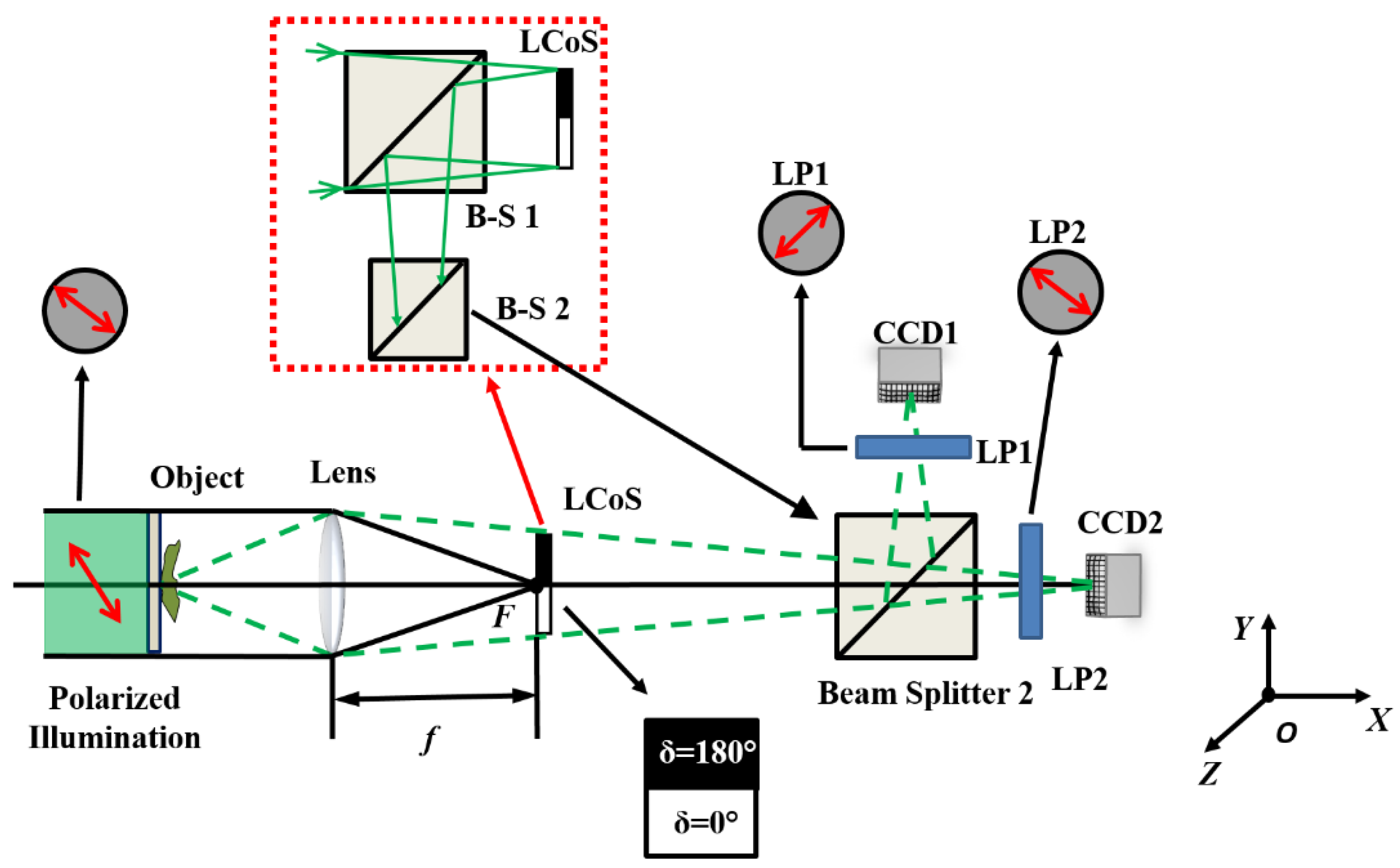
2.1. LCoS Display Self-Calibration

In order to optimally apply any LCoS display into a wavefront modulation system, the characteristic parameters of the LCoS display must be calibrated. A method for determining both the phase-voltage look-up table (Section 2.1.1) and the surface profile (Section 2.1.2) of the LCoS is following described.

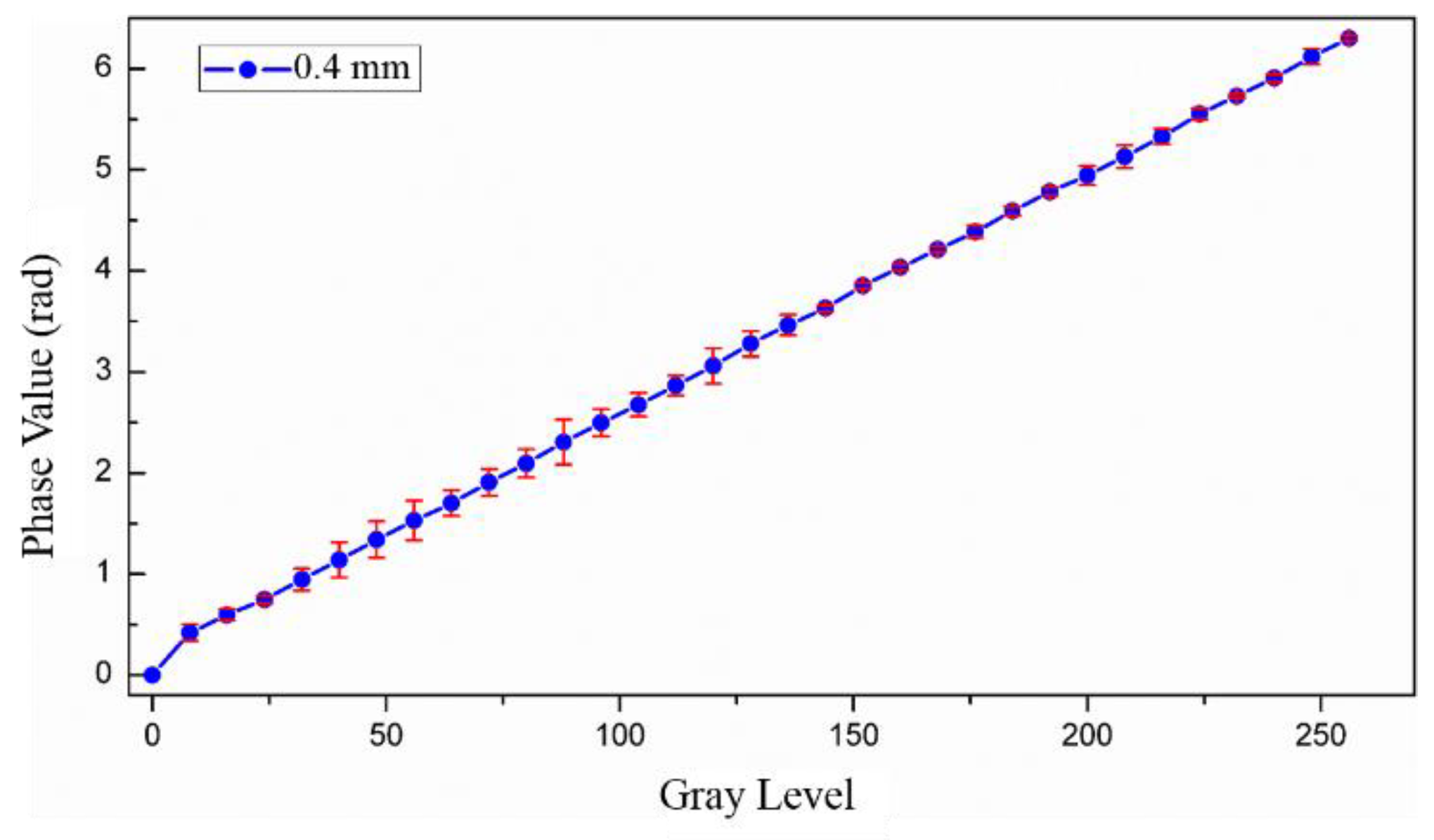
2.1.1. Phase-Voltage Calibration

We use an interferometric method, conducted by self-addressing a reconfigurable two-sectorial split-lens scheme on the LCoS display to be calibrated, to determine its phase-voltage response [15].

The two-sectorial split-lens configuration applied here represents the classic Billet lens scheme [30], which leads to an interference pattern equivalent to that of the Young’s double slit experiment. The optical scheme of this method is sketched in Figure 1. The Billet lens scheme consists of a lens cut from its center into two sections and then being separated with a certain distance (Figure 1b). The phase distribution of the digitally generated split-lens scheme, to be addressed to the LCoS display, is depicted in Figure 1a. Under this scenario, the coherent light illuminating the two-sectorial split-lens configuration at the LCoS plane generates two corresponding focal points (F1 and F2) at the focal plane (S plane in Figure 1). These two focal points act as new coherent and punctual light sources. Later, these two divergent beams further propagate and finally encounter at plane B, where a fringes-like interferometric pattern is produced (Figure 1c).

Once the interferometry pattern is obtained, the phase-voltage relation can be retrieved. To better explain this method, let us review the mathematical expression describing the two split-lens phase distribution shown in Figure 1a. This is given in Equation (1).

$$U_{N=2}(r,\theta )=U_1+U_2,$$

(1)

where U₁ and U₂ are the phase distribution for each one of the two lens sectors and they are written as [15],

$$U_1=\exp [i\frac{\pi }{\lambda f}(r^2+a_0{}^2-2r{a}_0\cos ({\theta }_i-{\theta }_0)+\varphi (V))],$$

(2)

$$U_2=\exp [i\frac{\pi }{\lambda f}(r^2+a_1{}^2-2r{a}_1\cos ({\theta }_{ii}-{\theta }_1))],$$

(3)

where f refers to the focal length of the split lens, r to the radial coordinate in the lens plane and λ represents the wavelength for the light source. In addition, a₀ is the distance from the first split-lens sector center to the LCoS geometric center, while a₁ is the distance from the second split-lens sector center to the same LCoS center. What is more, θ₀ and θ₁ refers to the angular positions of the two split sector centres. Thus, the upper sector angular distribution θ_i is restricted in the range as π to 2π, whereas the lower sector angular distribution θ_ii is restricted in the range as 0 to π. Note that these two sectors fully cover the whole angular distribution as 0 to 2π. Finally, note that the phase distribution for the first split sector (Equation (2)) introduces a constant phase term which depends on the voltage, $\varphi (V)$.

By setting a term $\varphi (V)$ different to zero in Equation (2) (each possible $\varphi (V)$ is related to a different gray level), a constant phase is added to one of the split sectors (U₁ in our case). This produces an extra retardance between wavefronts originated by U₁ and U₂, which is transferred into a transversal shift of the fringe pattern in a given axial plane (e.g., I plane). Therefore, by measuring the transversal shifts corresponding to the gray levels, the phase-gray levels relation can be determined, for instance, by using correlation-based calculations [22].

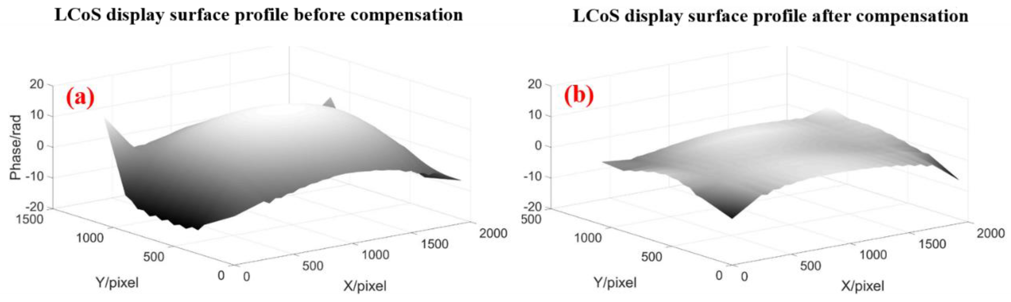
2.1.2. Surface Profile Calibration

To conduct the LCoS display surface calibration, a digital micro-lens array pattern (Shack–Hartmann scheme [19,20]) is self-addressed to the device. The micro-lens array consists of an ordered lattice of micro diffractive convergent lenses integrated at the LCoS plane. Moreover, all these lenses share the same focal length and the distance between any two adjacent lenses is equivalent. In this scenario, by sending the proper S-H phase distribution to the LCoS display, the diffractive micro-lens array is created. Let us assume now that we illuminate the LCoS with a collimated beam perpendicular to the display. In the case of a perfectly flat LCoS display surface (i.e., the screen does not introduce any extra phase distribution), we would obtain a uniformly distributed spot light configuration at the focal plane of the micro-lenses. In other words, each fraction of the input plane wave is focused at the optical axis of its corresponding micro-lens (see Figure 2a). On the contrary, if the LCoS screen presents spatial defects, the plane input wave is spatially distorted, and an extra phase distribution is added to the system, in a situation equivalent to Figure 2b. In such a scenario, corresponding spot lights at the focal plane are not evenly distributed but presents some deviation from the expected centers. Finally, by calculating the deviations of light dots with respect to the expected centers (see Figure 2b), the surface profile can be retrieved by using proper numerical methods.

We determine the light spot deviations by using centroid calculations thoroughly described in Ref. [20]. The main idea is to use a reference grid at the charge-coupled device (CCD) plane that indicates the theoretical centers. In particular, this reference grid corresponds to a system free of aberrations (light distribution at the focal plane related to a plane wave). Later, this grid is regarded as the criteria and the actual deviations of light dots observed when illuminating the LCoS, are estimated with respect to this reference grid. By determining such deviation, well-known integration methods [31] are used to retrieve the surface of the LCoS.

Two problems may arise by using this approach. First, we may introduce a reference grid pattern which is shifted from the theoretical grid. This situation leads to a constant shift into the centroid calculation. Nevertheless, this issue is easy to solve as in fact such grid shift can be regarded as a constant value added to the deviation function, and therefore, it only introduces an artificial tilt after using integration methods. Therefore, this situation does not modify the calculated surface profile. Conversely, we may face a second problem. If the size of the grid squares we choose is different from the theoretical one, linear phases are introduced into the centroid calculation and thus, a quadratic function is added to the surface profile after reconstruction during the integration. Therefore, the size of the grid has to be correctly determined as an input parameter to properly retrieve the LCoS surface profile. To solve this situation, we used the grid size calibration method discussed in Ref. [15]. Once the theoretical grid is properly set, experimental light spot deviations are measured with respect to theoretical centers. At this point, we can easily calculate the derivative function (slopes of the actual surface) from shifted light spots and then retrieve the surface profile by simply using the two-dimensional integration. At last, we use cubic splines [31] to interpolate discrete data and obtain a continuous surface profile.

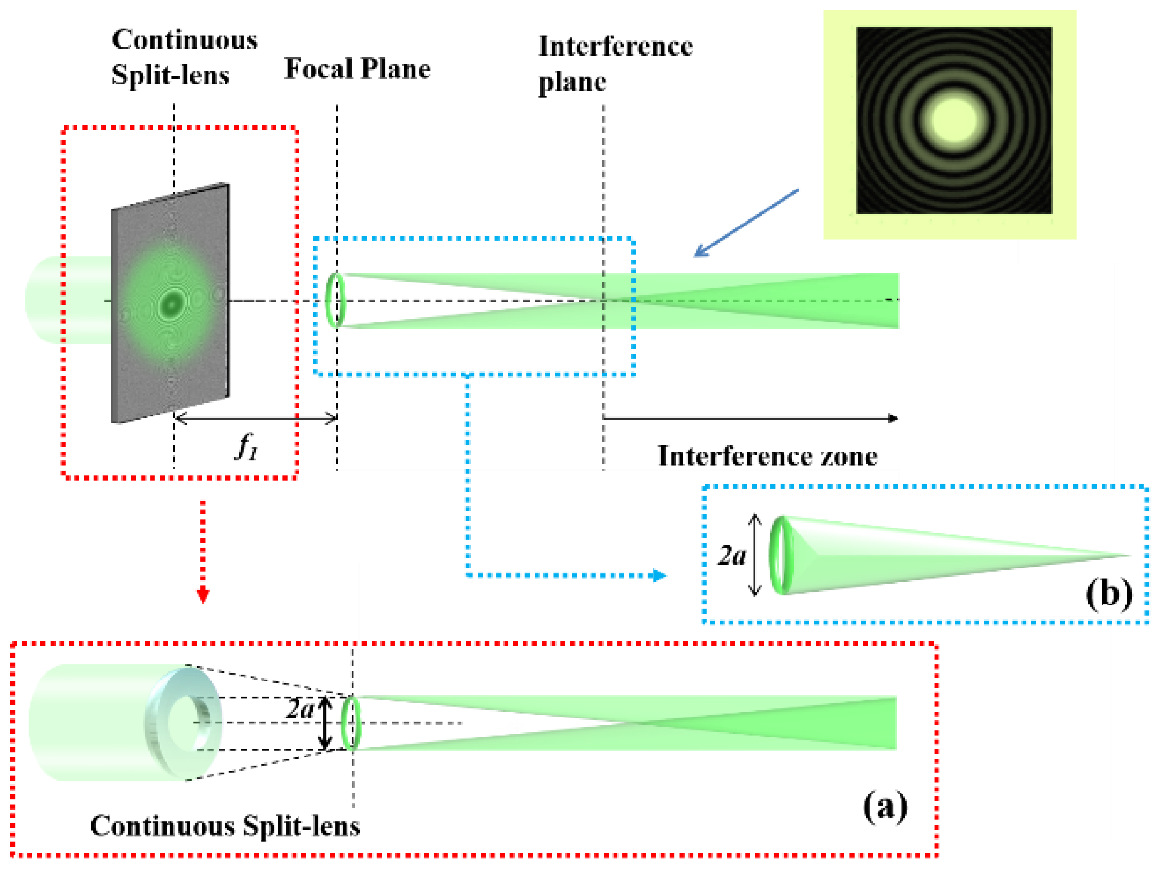
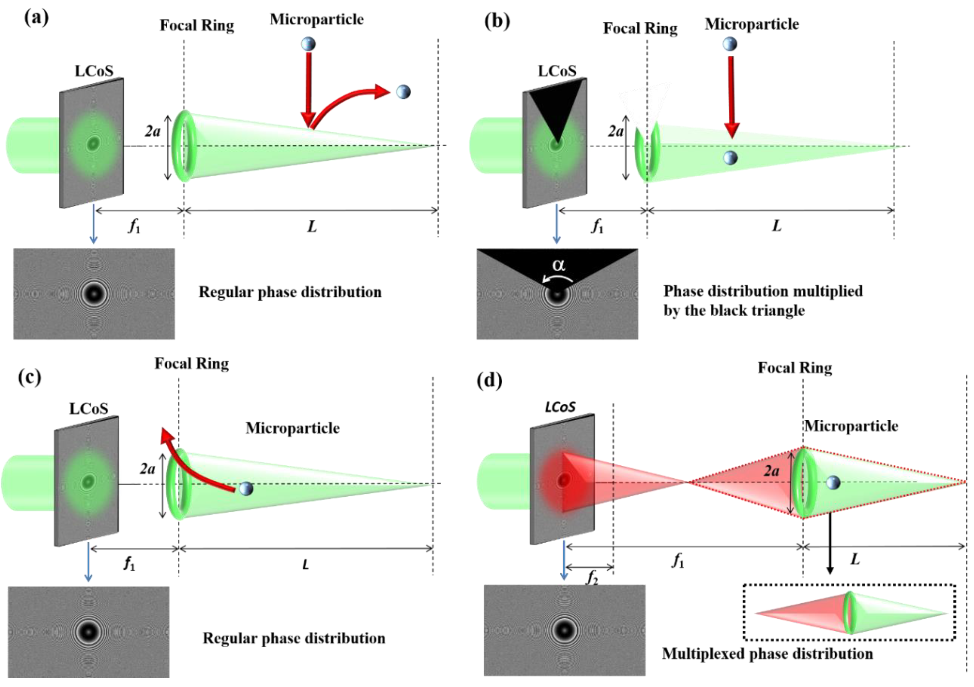
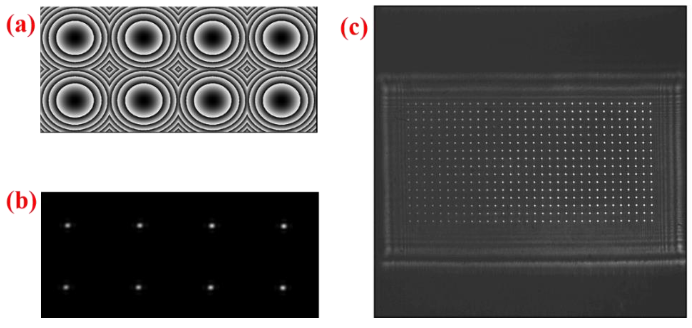
2.2. Microparticle Manipulation through Light Structures Created by a LCoS Display

We also present a method for microparticle spatial manipulation based on an LCoS display [12]. Before particle manipulation, they are firstly optically trapped into a three-dimensional light structure (optical bottle structure). These light structures are created thanks to the split-lens inspired configuration addressed to the LCoS. The physical mechanism that guarantees the particle trapping is here explained. The particle heated by the optical bottle structure experiences an opto-thermal force (photophoretic force [25]) with its force direction opposite to the gravity. Therefore, once the gravity of the particle is compensated by the photophoretic force, the particle is suspended in the air.

To obtain the reliable, easy-implemented light trapping architecture, we send to the LCoS display a digital diffractive N-sector based spilt-lens pattern [30,32]. This N-sector split-lens scheme shares the same principle as the Billet lens but this split-lens is adjusted to more pieces rather than the simple two pieces. The generated N-lens sectors are all separated the same distance to the center and share the same focal length. Therefore, we obtain diverse focal points drawing a circle at the focal plane. In particular, if the number of sectors is sufficient enough, a continuous split-lens configuration is created, which leads to a light ring at the focal plane. The configuration of such scheme is depicted in Figure 3.

In Figure 3, the input light modulated by the continuous split-lens phase distribution is propagated to the focal plane and the complete light ring (green ring) is obtained. Note that the continuous split-lens digital scheme is analogous to a classical lens continuously split and displaced from its center, as depicted in Figure 3a. In addition, a detail of the light cone trapping structure created by using this scheme is depicted in Figure 3b. In particular, light propagation after the light ring creates a hollow light cone that can be used as a basic structure for particle trapping. After the created light cone, interference between beams coming from different positions at the light ring occurs, and a Bessel beam structure is obtained (see the upper right corner in Figure 3).

To achieve the above-discussed light cone structure, the particular phase distribution to be sent at the LCoS display is given by Equation (4),

$$U(r,\theta )=\exp [i\frac{\pi }{\lambda f}{(r-a(\theta ))}^2]$$

(4)

where λ is the wavelength of the input light and f is the focal length shared by all the split-lens. Moreover, we define the phase distribution in the polar coordinate system (r, θ). Finally, we use a(θ) to describe the distance from the split lens to the LCoS coordinate origin.

By using the above-described scheme, we can effectively adjust some light cone characteristics (i.e., the cone length or its spatial position) by simply changing the focal length of the split-lens or the separation distance between the split-lens sectors. In particular, the length of the created light cones can be calculated by using Equation (5), according to geometrical optics relations,

$$L=a(\theta )f/\varphi$$

(5)

where $\varphi$ is the diameter of the generated continuous lens without being spilt (the lens aperture).

At this moment, we explain how to trap microparticles inside the light cone. By using the light cone shown in Figure 3, the particle cannot fall into the light cone because of its upper surface also offers photophoretic forces that bounces the particle away before entering into the light cone central space. This is demonstrated in Figure 4a. Therefore, we have to open the light cone structure from the upper section to allow particles entering its central area. Note that to open the light cone means removing light from the upper section. This is practically reliable just by properly multiplying an angular sector to the continuous split-lens phase distribution to be sent at the LCoS display. The angular sector presents a constant phase value and therefore, light illuminating this section on the LCoS display is not being modulated according to the split-lens scheme. Under this scenario, an opening is obtained in the light cone (see Figure 4b). Once the particle enters the light cone through the upper opening, we close the light cone from the top once again, by simply removing the added angular sector and recovering the original split-lens phase distribution. After this process, the microparticle is located into the light cone (see Figure 4c). Nevertheless, we still face one major problem as even though the particle is kept steady in the vertical direction, it is still not stable within the horizontal direction, as it can escape from the light cone front side (i.e., from the light circle plane, see Figure 4c). Thus, this section has to be closed to prevent particles from escaping. This is achieved by multiplexing a regular lens together with the continuous split-lens scheme. By choosing a focal length, for the regular lens, shorter than the distance between the LCoS and the light ring plane, light modulated by the regular lens acts as an stopper at the cone opened side (see effect of the regular lens represented by red light in Figure 4d). At this moment, a more sophisticated light structure, demonstrated as an optical bottle architecture, is realized within the combination of these two diffractive elements (regular lens and continuous split-lens). Under this scenario, the particle inside the light cone is now stably trapped within the new optical bottle as both sides are sealed. This optical bottle structure is demonstrated in Figure 4d. Last but not least, by simultaneously adjusting the focal lengths for both light structures, the whole optical bottle structure can be spatially moved along the axial direction. By doing this, the trapped microparticle is dragged by the light system, and the spatially manipulation of microparticles is efficiently realized.

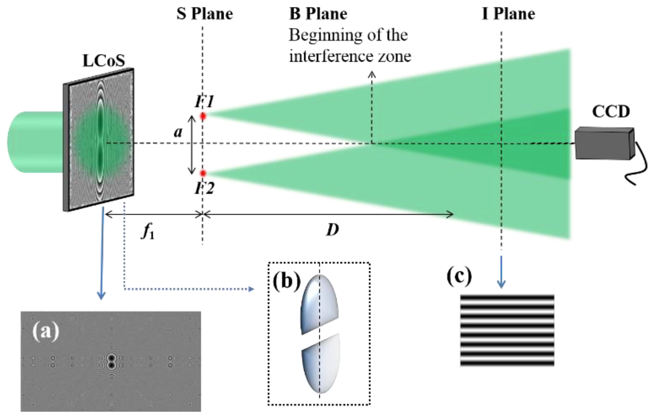
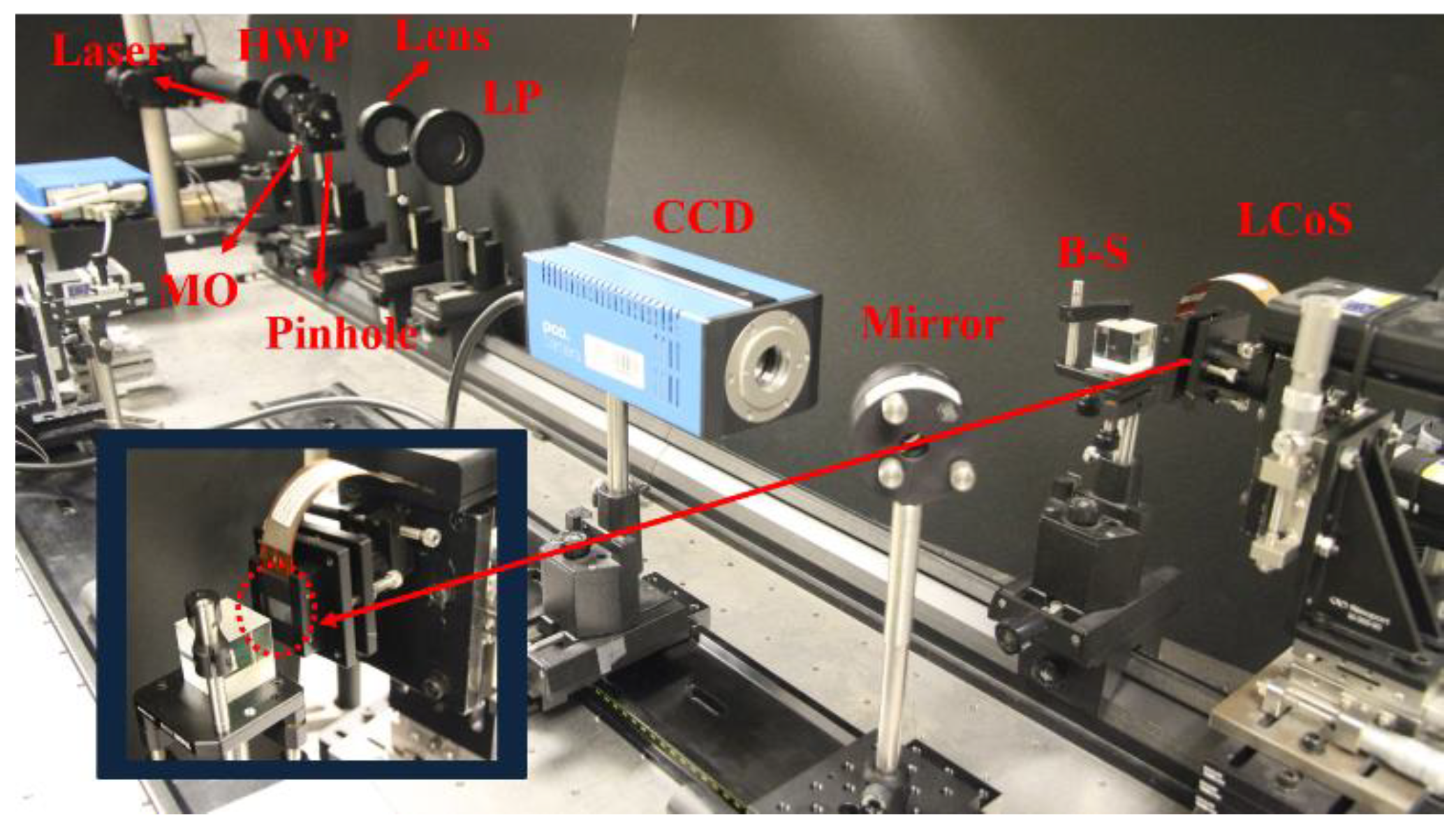
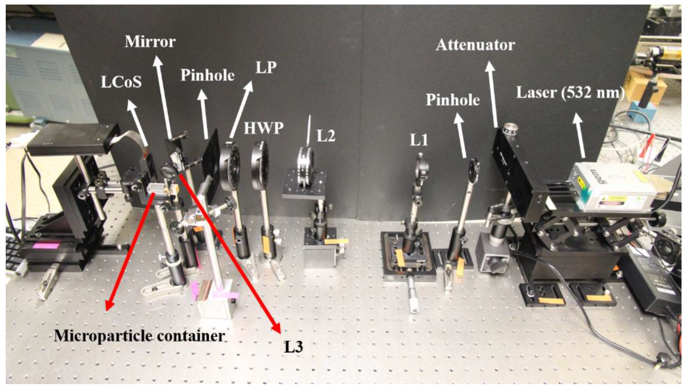
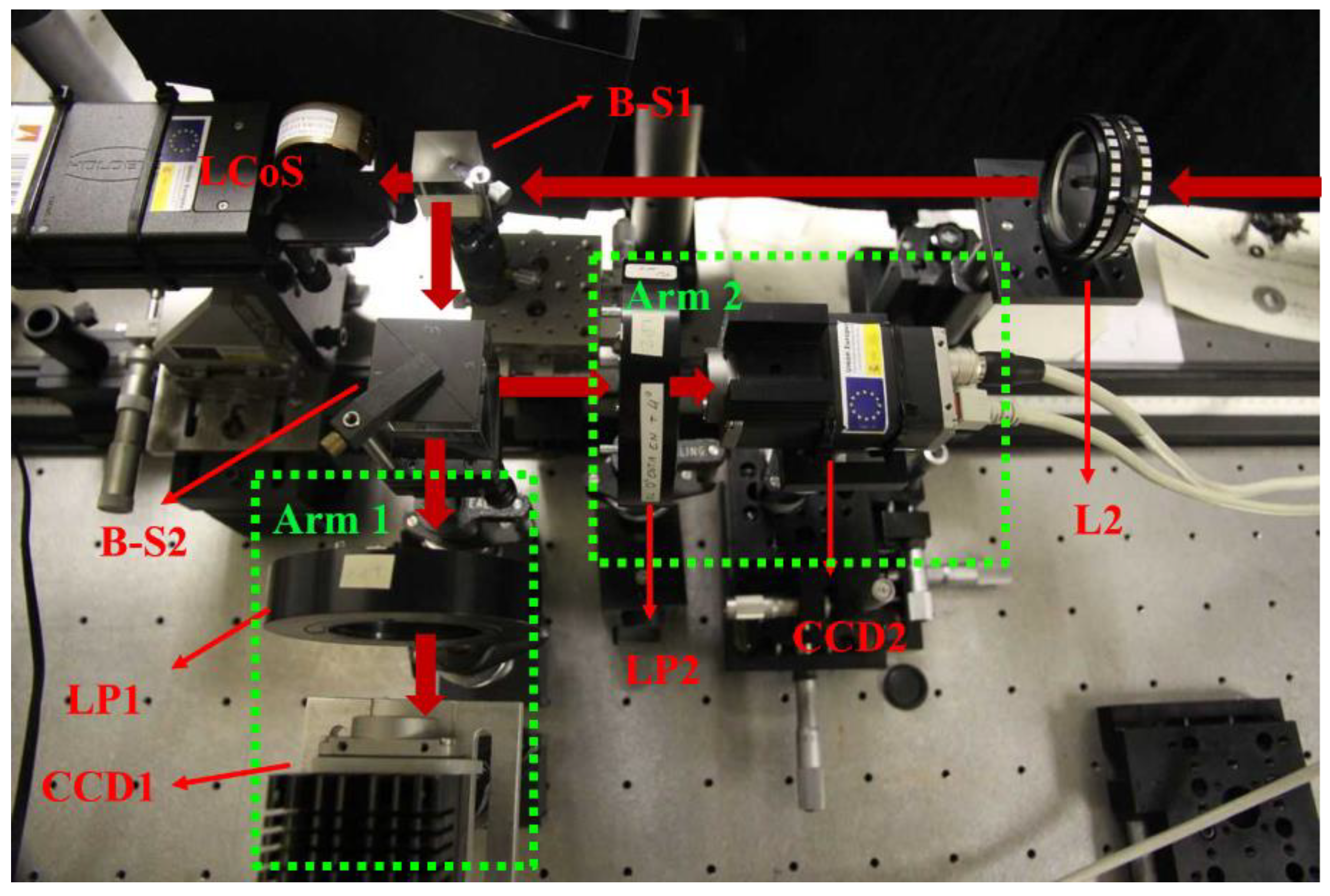
2.3. LCoS Display Based Inline Holographic System

In this section we introduce an inline (IL) holographic system to monitor particles in arbitrary spatial positions [23,24]. When performing holographic imaging of objects, the conjugate image (also referred as ghost image) is always added to the final image when dealing with inline holographic architectures, this situation dramatically deteriorating the image quality. To avoid this, off-axis set-ups for holographic imaging have been proposed in literature [33,34]. However, IL set-ups present some benefits when compared with off-axis set-ups, for instance, inline holographic systems provide a larger spatial bandwidth than off-axis systems [35].

An interesting proposal was given in Ref. [24,29], where the sideband technique was proposed for holographic imaging of objects, being able to remove ghost images into an IL system. The idea was to use a filter in the Fourier space to remove the contribution of the conjugate image. However, this filtering also removed object content, and the final image was degraded. We present in this section a double-sideband filter IL holographic system from which the undesired conjugate image is eliminated. More importantly, the full content of the object is retrieved, almost at real time, so it can be used for dynamic processes. To achieve the conjugate image removing, we implement the LCoS display as the digital double shutter.

To perform the double-sideband filtering, we firstly consider an almost transparent object (i.e., the microparticle with an extremely small diameter) and therefore, the wavefront passing through this object can be written as Equation (6),

$$U_o\left(x,y\right)=1+\Delta U_o\left(x,y\right),$$

(6)

where ΔU_o(x,y) refers to the small object amplitude variations. Thus, the Fourier transform of the wavefront amplitude distribution can be calculated as Equation (7),

$${\widetilde{{\displaystyle U}}}_o\left(\mu ,\nu \right)=\delta \left(\mu ,\nu \right)+\Delta {\widetilde{{\displaystyle U}}}_o\left(\mu ,\nu \right),$$

(7)

where δ represents the Dirac delta function, µ and ν refer to the spatial frequencies. The symbol ~ refers to the Fourier space.

Later, by implementing one section of the double-sideband filter at the Fourier plane, which is feasible to block the µ < 0 frequencies, we obtain the filtered wavefront amplitude at the image space (we refer it as CCD plane) as Equation (8) [29],

$$U_{CCD}^{+}=\frac{1}{2}+{\displaystyle \underset{0}{\overset{\infty }{\int }}\mathrm{d}\mu }{\displaystyle \underset{-\infty }{\overset{\infty }{\int }}\Delta {\widetilde{{\displaystyle U}}}_o\left(\mu ,\nu \right)e^{i2\pi \left(\mu x+\nu y\right)}\mathrm{d}\nu },$$

(8)

The intensity can be acquired as Equation (9) by calculating the square modulus of Equation (8),

$$\begin{array}{l}{I}_{CCD}^{+}={\left|U_{CCD}^{+}\right|}^2\approx \frac{1}{4}+\underset{{\mathrm{A}}^{+}}{\underset{\_}{\frac{1}{2}{\displaystyle \underset{0}{\overset{\infty }{\int }}\mathrm{d}\mu }{\displaystyle \underset{-\infty }{\overset{\infty }{\int }}\Delta {\widetilde{{\displaystyle U}}}_o\left(\mu ,\nu \right)e^{i2\pi \left(\mu x+\nu y\right)}\mathrm{d}\nu }}}\\ +\underset{{\mathrm{B}}^{+}}{\underset{\_}{\frac{1}{2}{\displaystyle \underset{-\infty }{\overset{0}{\int }}\mathrm{d}\mu }{\displaystyle \underset{-\infty }{\overset{\infty }{\int }}\Delta {\widetilde{{\displaystyle U}}}_{{}_o}^{*}\left(-\mu ,-\nu \right)e^{i2\pi \left(\mu x+\nu y\right)}\mathrm{d}\nu }}},\end{array}$$

(9)

where the fourth term which contained the small value of |$\Delta {\widetilde{{\displaystyle U}}}_o$|² is neglected considering the transparent assumption of the object.

The second term (A⁺) in Equation (9) only carries the positive frequencies µ > 0 of the object image, and on the contrary, the third term (B⁺) contains the negative frequencies µ < 0 of the conjugate image (note that asterisk * in the third term represents the complex conjugation). Finally, we digitally Fourier transform the obtained intensity (i.e., $I_{CCD}^{+}$ in Equation (9)), and the µ < 0 frequencies are removed. Under this scenario, the complex amplitude is calculated as Equation (10),

$${\left|U_{CCD}^{+}\right|}^2\approx \frac{1}{4}+\underset{{\mathrm{A}}^{+}}{\underset{\_}{\frac{1}{2}{\displaystyle \underset{0}{\overset{\infty }{\int }}\mathrm{d}\mu }{\displaystyle \underset{-\infty }{\overset{\infty }{\int }}\Delta {\widetilde{{\displaystyle U}}}_o\left(\mu ,\nu \right)e^{i2\pi \left(\mu x+\nu y\right)}\mathrm{d}\nu }}},$$

(10)

Note that by only addressing one sideband filter (which in fact is one section of the double-sideband filter), the undesired conjugate term (i.e., the B⁺ term in Equation (9)) is removed. However, the complex amplitude in Equation (10) cannot guarantee a complete wavefront reconstruction as the µ < 0 frequencies are missing. Therefore, a second sideband filter able to only filter the µ > 0 frequencies is addressed. As will be further explained, both sideband filters are simultaneously addressed thanks to the use of the LCoS display. The intensity obtained at the CCD plane by using this second filter can be calculated in a way equivalent to the above-stated filtering process, but now, by removing µ > 0 frequencies. It leads to the following expression Equation (11) [29],

$${\left|U_{CCD}^{-}\right|}^2=\frac{1}{4}+\underset{{\mathrm{A}}^{-}}{\underset{\_}{\frac{1}{2}{\displaystyle \underset{-\infty }{\overset{0}{\int }}\mathrm{d}\mu }{\displaystyle \underset{-\infty }{\overset{\infty }{\int }}\Delta {\widetilde{{\displaystyle U}}}_o\left(\mu ,\nu \right)e^{i2\pi \left(\mu x+\nu y\right)}\mathrm{d}\nu }}}.$$

(11)

The finally object image, containing the whole spatial frequency distribution of the quasi-transparent object, can be finally written as Equation (12) by combining Equations (10) and (11),

$$I={\left|U_{CCD}^{-}\right|}_{A^{-}}^2+{\left|U_{CCD}^{+}\right|}_{A^{+}}^2=\frac{1}{2}+\underset{{\mathrm{A}}^{-}}{\underset{\_}{\frac{1}{2}{\displaystyle \underset{-\infty }{\overset{0}{\int }}\mathrm{d}\mu }{\displaystyle \underset{-\infty }{\overset{\infty }{\int }}\Delta {\widetilde{{\displaystyle U}}}_o\left(\mu ,\nu \right)e^{i2\pi \left(\mu x+\nu y\right)}\mathrm{d}\nu }}}+\underset{{\mathrm{A}}^{+}}{\underset{\_}{\frac{1}{2}{\displaystyle \underset{0}{\overset{\infty }{\int }}\mathrm{d}\mu }{\displaystyle \underset{-\infty }{\overset{\infty }{\int }}\Delta {\widetilde{{\displaystyle U}}}_o\left(\mu ,\nu \right)e^{i2\pi \left(\mu x+\nu y\right)}\mathrm{d}\nu }}}=\frac{1}{2}{U}_0(x,y).$$

(12)

In Equation (12), we can clearly distinguish that the conjugate image is eliminated and therefore the object image is obtained without the distortions associated to ghost images. Once the full complex amplitude is assured (i.e., Equation (12)), the holographic wavefront image can be reconstructed at any axial plane by using some diffraction method. We used the Rayleigh-Sommerfeld diffraction method, and the reconstructed wavefront is given by Equation (13) [36,37],

$$U(x,y,d)={\displaystyle \iint \widetilde{{\displaystyle I}}\left(\mu ,\nu \right)\times \exp \{\frac{i2\pi }{\lambda }d{[1-{\lambda }^2({\mu }^2+{\nu }^2)]}^{1/2}\}}\times \exp [i2\pi (x\mu +y\nu )]\mathrm{d}\mu \mathrm{d}\nu ,$$

(13)

where Ĩ(µ,ν) is the Fourier transfer of Equation (12) and d is the axial distance from the image input plane to the particular position where we want to reconstruct the wavefront.

So far, we have theoretically discussed the mathematical background to implement the IL holographic wavefront imaging through a double-sideband filter. Here, an optical scheme to illustrate how the real implementation of such system can be conducted by using an LCoS display (as the digital double-sideband filter) is presented. The optical sketch is shown in Figure 5, where a polarized collimating light is used as the illumination with its polarization direction rotated 45° to Y-axis of the world coordinate system. Afterwards, a convergent lens is inserted after the tested object and therefore, we can determine the Fourier plane at its focal plane F. By now, the LCoS display is precisely implemented at the Fourier plane so that it can provide the frequency filtering. Even though that the spatial light modulator presented in Figure 5 is described as a transmissive element for the sake of clarity, in fact, it is the LCoS display working within the reflective scheme. The actual reflective configuration is conducted by combining the LCoS display with a beam splitter (it is also shown in Figure 5; see red dashed inset image). Into this LCoS display, we set two sectorial phase retardations: half of the display is driven to a phase of 0° and the other half to 180° (see Figure 5). Under this scenario, the polarization direction of the input light passing through the LCoS is rotated for 90° in the upper section (black section, δ as 180°), whereas on the contrary, the polarization direction corresponding to the other section (white section, δ as 0°) is maintained.

Later, two linear analyzers (LP1 and LP2) are set before the two CCDs cameras. Their transmissive directions are set perpendicular to each other: LP2 is oriented 45° to the Y-axis (the same polarization direction as the input light) and LP1 is oriented to 135° to the Y-axis. Under this scenario, the combination of the LCoS polarization modulation and the analyzers LP1 and LP2 orientations acts as the double sideband filter. Light recorded by CCD1 was previously filtered as half of the object frequencies are blocked. This can be assimilated to Equation (10). On the contrary, LP2 acts as a second filter and the wavefront recorded by the second CCD can be assimilated to Equation (11). Therefore, the final reconstructed holographic wavefront imaging of the object without the conjugate image can be achieved by considering Equation (13). Moreover, we want to note that such IL holographic system presents another advantage apart from the conjugate image removing as it is feasible to record dynamic processes, which is extremely favored for the study of particles in motion.

3. Results

The experimental implementation of the LCoS self-calibration is preliminarily presented in this section using the split-lens configuration as well the micro-lens array scheme (Section 3.1). Afterwards, in Section 3.2 we show the experimental particle trapping and manipulation, by using the method described in Section 2.2. Finally, in Section 3.3 we show the experimental implementation of the inline holographic system proposed in Section 2.3, and the practicability is verified by monitoring some dynamic microparticles.

3.1. LCoS Display Self-Calibration

In this subsection, we present the experiments to realize both the LCoS display phase-voltage and surface profile calibration.

3.1.1. Phase-Voltage Calibration

In this section, the method described in Section 2.1.1, is experimentally implemented and tested to determine the phase-voltage relation of the LCoS display. The sketch shown in Figure 1 is experimentally implemented and shown in Figure 6. We use a polarized He-Ne laser with the wavelength of 632.8 nm as the illumination. Later, light is expanded and collimated through the combination of a microscope objective (MO), a pinhole and a convergent lens. Note that the combination of such three elements not only makes light expansion feasible, but also they guarantee light filtering. A half-waveplate (HWP) combined with a linear polarizer (LP) is used to control the intensity of light illuminating the LCoS. In addition, the direction of LP is selected to ensure an LCoS display performance in the phase-only regime (i.e., the polarization direction is parallel to the LC director direction). Once the input light is properly modulated, the PLUTO-LCoS display (distributed by HOLOEYE) is aligned with its surface strictly perpendicular to the input beam (see the zoomed figure at the right bottom corner of Figure 6). Here, the LCoS display presents a 1920 × 1080 resolution with the pixel size as 8 µm, and it has the filling factor as 87%. Finally, the collimated light entering the LCoS display is modulated by the digital two split-lens configuration (see Figure 1a) and the corresponding fringes-like interference pattern is obtained at the CCD camera, with the help of the beam splitter (B-S) and the mirror placed after the LCoS.

Once the system set-up is determined, the two split-lens configuration is addressed to the LCoS display. The focal length of the addressed split-lens is set to 350 mm and the separation distance as 0.4 mm. Later, the two split-lens scheme is addressed for different values of the constant phase $\varphi (V)$, so that the interferometry pattern is modified (see Section 2.1). To realize the whole gray level range calibration, we drive different voltages (phases) by the means of changing the gray level from 0 to 255 with the step of 8. Therefore, 33 different interferometry patterns are obtained in the CCD with each pattern relates one phase value (voltage) to its corresponding gray level. As stated in Section 2.1, from this collection of interference patterns, the phase-voltage look-up table can be retrieved [22]. The obtained experimental curve, representing the phase as the function of the gray level, is shown in Figure 7. Each data in the curve given in Figure 7 is obtained by repeating the experiment for one hundred times, hence we also calculate the corresponding standard deviations, which are presented as the error bars in red. From Figure 7, we see that the phase-gray level curve demonstrates a nearly linear distributed tendency and the error bar values along the whole distribution are small. What is more, the phase values after the calculation is ranging from 0 to ~6.28 radians, which is suitable for phase-only applications.

3.1.2. Surface Homogeneity Calibration

The surface homogeneity calibration shares the same experimental set-up given in Figure 6, and it is achieved just by changing the phase pattern addressed to the LCoS display. In this case, the Shack–Hartmann configuration is addressed (see Section 2.1.2). In particular, we generate a 4 × 2 micro-lens pattern in which each micro-lens scheme occupies 400 × 400 LCoS pixels. Therefore, the whole micro-lens scheme presents an LCoS display dimension as 1600 × 800 pixels. The phase distribution of such scheme is given in Figure 8a and the corresponding spot-array received at the focal plane is given as Figure 8b. Note that such eight micro-lenses pattern cannot cover the whole LCoS surface, not to mention so few focal points cannot guarantee a precise surface integration [31]. Therefore, we dynamically displace the generated micro-lens pattern along the whole LCoS screen both in x and y directions. In both directions, this is implemented for 8 times with a step of 50 pixels. Finally, by recording the 8 focal points within each step (64 displacements in total) we can construct a full image with 512 intensity spots in the CCD (see Figure 8c). Once the final spot array image is obtained, we implement a 38 × 38 reference grid to analyze the spot deviations from their corresponding centers.

As detailed in Section 2.1.2, by calculating the deviations of light dots in the final spot array image (i.e., image in Figure 8c) from a reference pattern, the final LCoS surface can be reconstructed. Obtained results are given in radian units in Figure 9a, where a quadratic profile is clearly observed. This quadratic deformation is normally introduced by the lateral mechanical stress applied on the screen during the fabrication process, when the LC surface is stuck to the bottom structures of the LCoS display. To describe the quadratic profile of the LCoS display quantitatively, we studied the pixel-value cross section of a horizontal line in Figure 9a (from the middle pixel of the surface left edge to the middle pixel of the surface right edge). The corresponding peak-to-valley (PV) value of such line is 28.01 radians. To compensate such quadratic deviation, we implement a further step by adding the inverse phase distribution of Figure 9a to the LCoS display. Under this scenario, we repeated the LCoS surface measurement, once again by using the same self-addressed S-H scheme. Ideally, the screen profile after such compensation should be flat. In reality, the measured compensated surface profile after correction is given in Figure 9b, where we can easily find the quadratic error is almost eliminated, and the obtained surface is smoother. In particular, the surface PV (for the same pixels line previously stated) after correction is decreased to just 1.28 radians.

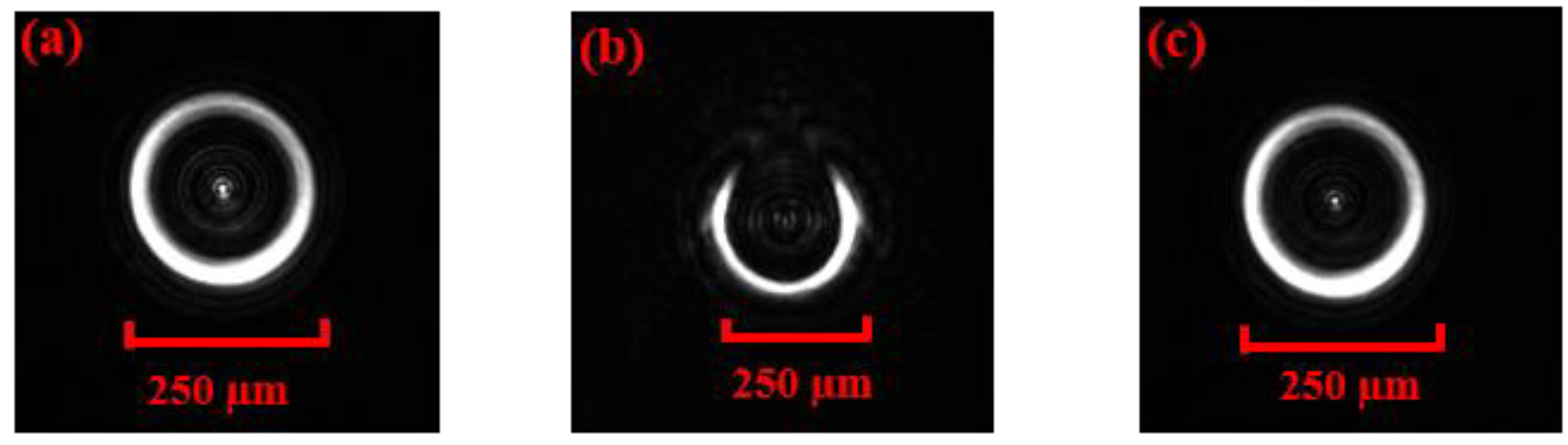
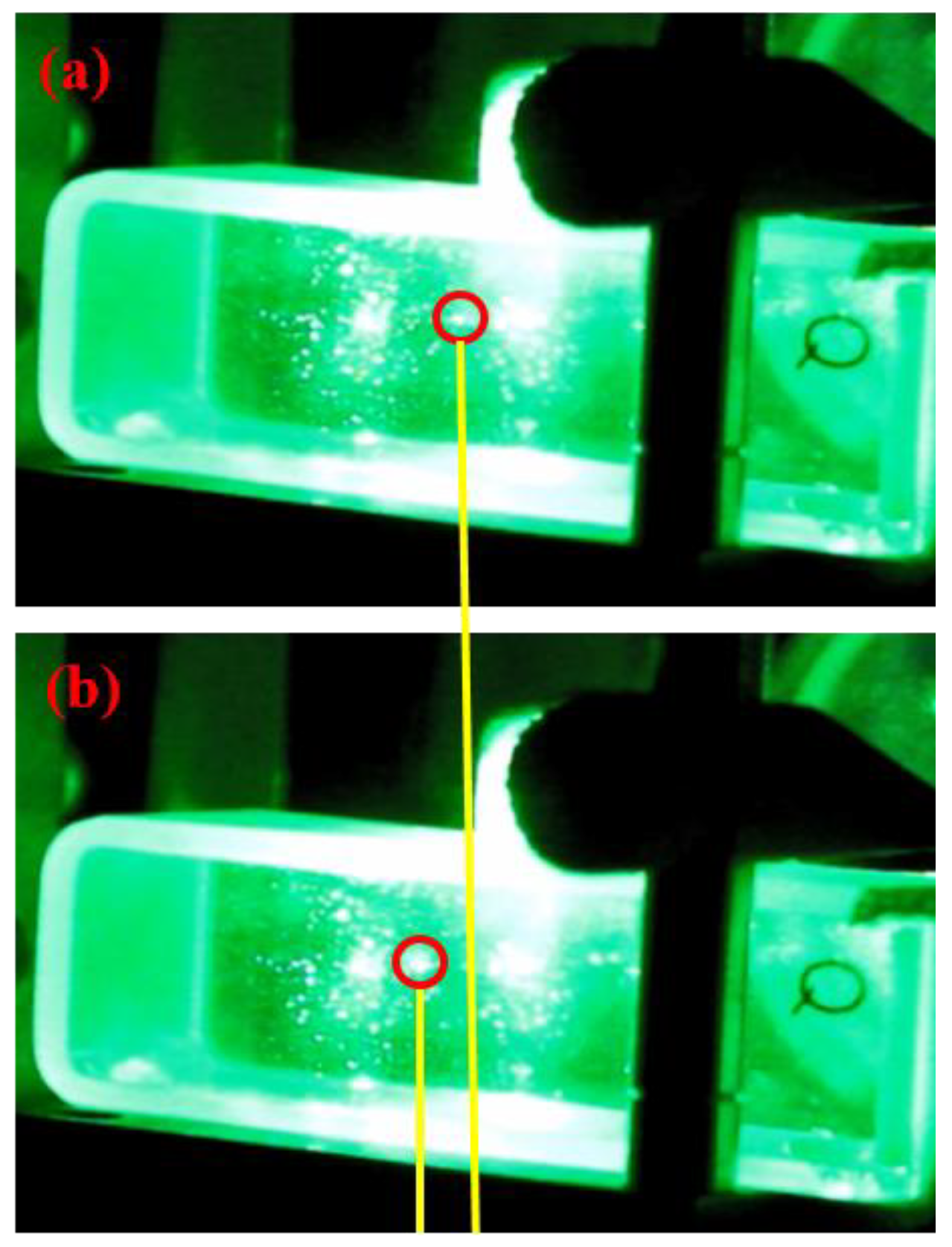
3.2. Microparticle Manipulation through the LCoS Display Generated Split-Lens Schemes

In this subsection, we implement the method described in Section 2.2 to create a customized three dimensional light capsule to capture and spatially manipulate microparticles. The optical set-up implemented to such aim is given in Figure 10.

The system is illuminated with a 532 nm wavelength laser (gem 532 Model, Laser Quantum) with the output power ranging from 50 mW to 2 W. Afterwards, one attenuator combined with a pinhole is inserted into the system to properly adjust the intensity. Then, light passing through an afocal system, formed by a divergent lens (L1, f₁ as −100 mm) and a convergent lens (L2, f₂ as 300 mm), is collimated and expanded. Next, the LCoS display is located perpendicular to the input beam. A linear polarizer (LP) placed before the LCoS is properly oriented to ensure a phase-only performance of the device. Under this scenario, we send two multiplexed phase distributions to the LCoS display: (i) the first one defines the continuous split-lens configuration (creates the light cone); and (ii) the second stands for a regular lens (configures the cone cork). See more details in explanation related to Figure 4. Specifically, the parameters set to implement the continuous split-lens are: the distance between sector centers to the origin of a = 1.07 mm, a focal length of f = 370 mm and an aperture of $\varphi$ = 2.07 mm (see Equations (4) and (5)). Conversely, the focal length for the regular lens is set 350 mm. Note that in this scheme, the focal length of the regular lens (i.e., 350 mm) is smaller than the continuous split-lens (i.e., 370 mm) which satisfies the structure described in Figure 4d. Finally, a convergent lens (L3) images the whole structure into a transparent container, in which a number of microparticles are stuck to the top face due to electrostatic forces. By taking into account all these experimental parameters, we have obtained an experimental optical bottle with an axial length of ~6.5 mm. Now, this compacted optical bottle is feasible to capture particles through photophoretic forces. The used transparent container is a square UV fused quartz cuvettes (Thorlab CV10Q3500) with its size of 45–10–10 mm and two sides polished. On the other hand, the used particles are carbon coated hollow glass microspheres (Cospheric HGMS-0.14 63–75 µm) with their diameters ranging from 63–75 µm. Moreover, the particle density is 0.14 g/cm³ and the mass ranged from 18.3–30.9 ng. Here, we want to note that apart from the carbon coated microsphere, the pure carbon particles [36] or the absorbing silicon particles [37] are also feasible to be trapped. As told before, particles are preliminarily stuck to the container inner surface by electrostatic forces. At this moment, these particles are not able to enter into the optical bottle structure because light capsule is sealed. The central cross section figure corresponding to this light capsule structure is given in Figure 11a. However, optical bottle can be opened from the top by multiplying an azimuthal sector with a constant phase within the continuous lens phase distribution, as detailed in Section 2.2. As a consequence, the resulting central cross section is provided in Figure 11b, this scheme enabling particles to enter into the light structure. By softly tapping the above side of the container, we forced particles to land into the capsule and they can be trapped by photophoretic forces exerted by the light structure. Finally, we closed the upper section of the light structure once again, by removing the triangle gap, and the complete optical bottle was recovered (see Figure 11c). Once the optical bottle is sealed, the particle is stably contained into this light structure. The particle trapped in this optical bottle is demonstrated in Figure 12a where we highlight the spatial particle position with a red circle.

Apart from the fact that we are able to trap particles in the generated optical bottle, we also moved a step further by implementing the particle manipulation. This is achieved by changing the spatial position of the optical bottle itself. To be more specific, we simply changed the focal length of the digital split-lens from 370 mm to 381 mm, and we also modified the focal length of the digital regular lens from 350 mm to 361 mm. By taking into account Equation (5), the optical bottle length was correspondingly changed from the original ~6.5 mm to the current ~5.35 mm. Moreover, due to the modification of the focal length values, the optical bottle was spatially shifted for ~0.47 mm in the optical axis direction. As the optical bottle is moved, the particle trapped inside is spatially dragged in the same shifting direction. Therefore, we can control the axial position of the particle. The axially shifted particle is demonstrated in Figure 12b, where the displacement can be discovered from the spatial difference compared to Figure 12a (i.e., the original trapped particle).

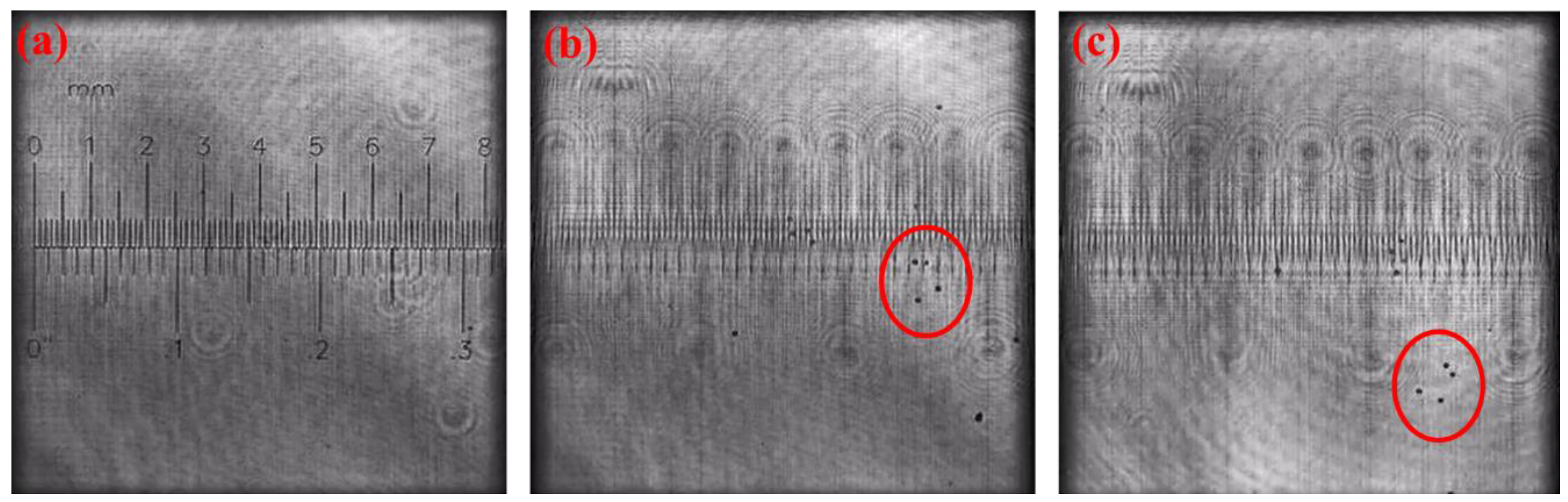
3.3. LCoS Display Based Inline Holographic System

In this section, we present the experimental implementation to achieve the IL holographic imaging using the LCoS display (see Section 2.3 and Figure 5). The experimental implementation is shown in Figure 13. We use as illumination a 633 nm wavelength linear polarized laser with the output power as 17 mW. The laser is then spatially filtered and later collimated by a convergent lens L1 (focal length as 250 mm). The object to be studied is placed to a distance after L1. Then, we insert a second convergent lens with a focal length of 300 mm (L2, see Figure 13). The function of L2 is twofold: one the one hand, it images a plane of the object space (we label it as object plane P) into the CCD1 and CCD2 camera planes (the object plane was situated at 690 mm before L2); on the other hand, the Fourier spectrum of the object is set at the focal plane of L2, where the LCoS display is set. Note that this configuration accomplishes the scheme shown in Figure 5.

As the LCoS used (distributed by HOLOEYE) works into a reflective configuration, a system of beam-splitters (B-S1 and B-S2 in Figure 13) are used to properly imaging the object to CCD1 and CCD2. What is more, the obtained images at the CCDs are filtered according to the double-sideband filter explained in Section 2.3. This is experimentally achieved thanks to combination of the LCoS display with two linear polarizers (LP1 and LP2 in Figure 13), which are placed in front of the CCD1 and CCD2 cameras, respectively. As CCD cameras we used two Basler CCDs (KAI-1020) which guarantee the resolution of 1MP with the frame rate as 60 fps. Note that for a better vision, the optical elements before the second convergent lens (i.e., the laser, the primary convergent lens and the spatial filter) are ignored in Figure 13.

By computational processing the images recorded by CCD1 and CCD2, according to the mathematical formulation described in Section 2.3, holographic images of objects can be retrieved without the degradation associated to ghost images. In particular, we implemented two objects for the measurement at the same time: a reticle and a thin glass plate. In the case of the thin glass plate, it is covered with microparticles with sizes of ~100 µm. The reticle is located 50 mm before the P plane (i.e., 740 mm before L2) and the thin glass plate with microparticles is implemented closer to L2, 50 mm behind the P plane (i.e., 640 mm before L2). In this way we can prove how we simultaneously image the reticle and the microparticles, which are at different axial planes. Moreover, the thin glass plate is hinged to a rotation mechanism from which we can provide the dynamic potential of the method.

By applying the method explained in Section 2.3 we can reconstruct the complex amplitude at the object plane P. From this information, reticle and thin glass plate can be also retrieved by properly applying the Rayleigh-Sommerfeld diffraction method (Equation (6)) [38,39]. In particular, by taking into account the magnification introduced by L2, the reticle plane is reconstructed by setting the reconstruction position of z = −30 mm to the object plane P (note P is set at z = 0). Results are given in Figure 14a, where the image of the reticle is clearly distinguished but the microparticles are defocused (see Figure 14a). Afterwards, by changing the reconstruction position to z = +31 mm, we focus the microparticles plane (microparticles on the thin glass plate) but the reticle at this time is defocused (see Figure 14b). Such pattern shifting demonstrates the feasibility of using the IL holography system to realize the object imaging at different axial positions. Finally, we rotated as well the thin glass plate from which we observed the microparticle dynamic rotation. The rotated microparticles are presented in Figure 14c from which the position shifting compared to Figure 14b is clearly demonstrated.

4. Conclusions

We reviewed different techniques we recently proposed to calibrate and apply LCoS display technology. We preliminarily use a self-calibration method to determine the phase-gray level relation and the surface profile of an LCoS display. In particular, the phase-voltage relation is experimentally determined by using the diffractive split-lens configuration. Such method leads to an interferometric pattern that is transversally displaced as a function of the gray level. From this relation, the phase-gray level curve is accurately determined. On the other hand, by using the same optical arrangement, but addressing a different self-addressed hologram (in this case, the Shack–Hartmann scheme), we are able to determine the LCoS screen profile. From this information, the effect of the screen distortions was corrected, reaching a higher performance of the device. Afterwards, this calibrated LCoS display was implemented into an optical set-up able to trap and manipulate microparticles. To this aim, three-dimensional light structures were created by using split-lens based configurations. The created structures configured an optical bottle, where some particles (glass coated microspheres) were experimentally trapped. Moreover, by simply modifying some control parameters, we conducted the spatial shifting of the optical bottle in the axial direction, which allowed us to control the spatial position of the captured particle. Finally, a method to obtain holographic images of objects was also described. This is an inline (IL) holographic system based on an LCoS display. The method shares all the benefits of inline schemes, but avoids one major problem associated to IL systems, the non-desired influence of ghost images. This is achieved by implementing a double-sideband filter (DSF) at the Fourier plane of the object. The DSF is implemented thanks to the combination of the LCoS display with a pair of linear analyzers. We experimentally demonstrated how the method is able to eliminate the unsatisfied conjugate image. What is more, this LCoS based IL holographic scheme avoids the necessity of time-sequential measurements and therefore, we achieved the dynamic holographic observation.

References

1. Mu, Q.; Cao, Z.; Hu, L.; Li, D.; Xuan, L. Adaptive optics imaging system based on a high-resolution liquid crystal on silicon device. Opt. Express 2006, 14, 8013–8018. [Google Scholar] [CrossRef] [PubMed]
2. Fernández, E.J.; Prieto, P.M.; Artal, P. Wave-aberration control with a liquid crystal on silicon (LCOS) spatial phase modulator. Opt. Express 2009, 17, 11013–11025. [Google Scholar] [CrossRef] [PubMed]
3. Zhang, Z.; You, Z.; Chu, D. Fundamentals of phase-only liquid crystal on silicon (LCOS) devices. Light Sci. Appl. 2014, 3, e213. [Google Scholar] [CrossRef]
4. Matsumoto, N.; Itoh, H.; Inoue, T.; Otsu, T.; Toyoda, H. Stable and flexible multiple spot pattern generation using LCOS spatial light modulator. Opt. Express 2014, 22, 24722–24733. [Google Scholar] [CrossRef] [PubMed]
5. Marquez, A.; Moreno, I.; Iemmi, C.; Lizana, A.; Campos, J.; Yzuel, M.J. Mueller-Stokes characterization and optimization of a liquid crystal on silicon display showing depolarization. Opt. Express 2008, 16, 1669–1685. [Google Scholar] [CrossRef] [PubMed]
6. Ni, J.; Wang, C.; Zhang, C.; Hu, Y.; Yang, L.; Lao, Z.; Xu, B.; Li, J.; Wu, D.; Chu, J. Three-dimensional chiral microstructures fabricated by structured optical vortices in isotropic material. Light Sci. Appl. 2017, 6, e17011. [Google Scholar] [CrossRef] [PubMed]
7. Kowalczyk, A.P.; Makowski, M.; Ducin, I.; Sypek, M.; Kolodziejczyk, A. Collective matrix of spatial light modulators for increased resolution in holographic image projection. Opt. Express 2018, 26, 17158–17169. [Google Scholar] [CrossRef] [PubMed]
8. Fuentes, J.L.M.; Moreno, I. Random technique to encode complex valued holograms with on axis reconstruction onto phase-only displays. Opt. Express 2018, 26, 5875–5893. [Google Scholar] [CrossRef] [PubMed]
9. Vinas, M.; Dorronsoro, C.; Radhakrishnan, A.; Benedi-Garcia, C.; Lavilla, E.A.; Schwiegerling, J.; Marcos, S. Comparison of vision through surface modulated and spatial light modulated multifocal optics. Biomed. Opt. Express 2017, 8, 2055–2068. [Google Scholar] [CrossRef] [PubMed]
10. Qaderi, K.; Leach, C.; Smalley, D.E. Paired leaky mode spatial light modulators with a 28° total deflection angle. Opt. Lett. 2017, 42, 1345–1348. [Google Scholar] [CrossRef] [PubMed]
11. Cheng, Q.; Rumley, S.; Bahadori, M.; Bergman, K. Photonic switching in high performance datacenters [Invited]. Opt. Express 2018, 26, 16022–16043. [Google Scholar] [CrossRef] [PubMed]
12. Lizana, A.; Zhang, H.; Turpin, A.; Van Eeckhout, A.; Torres-Ruiz, F.A.; Vargas, A.; Ramirez, C.; Pi, F.; Campos, J. Generation of reconfigurable optical traps for microparticles spatial manipulation through dynamic split lens inspired light structures. Sci. Rep. 2018, 8, 11263. [Google Scholar] [CrossRef] [PubMed]
13. Zhang, H.; Lizana, A.; Van Eeckhout, A.; Turpin, A.; Iemmi, C.; Márquez, A.; Moreno, I.; Torres-Ruiz, F.A.; Vargas, A.; Pi, F.; et al. Dynamic microparticle manipulation through light structures generated by a self-calibrated Liquid Crystal on Silicon display. Proc. SPIE 2018, 10677, 106772O. [Google Scholar] [CrossRef]
14. Fuentes, J.L.M.; Fernández, E.J.; Prieto, P.M.; Artal, P. Interferometric method for phase calibration in liquid crystal spatial light modulators using a self-generated diffraction-grating. Opt. Express 2016, 24, 14159–14171. [Google Scholar] [CrossRef] [PubMed]
15. Zhang, H.; Lizana, Á.; Iemmi, C.; Monroy-Ramirez, F.A.; Márquez, A.; Moreno, I.; Campos, J. LCoS display phase self-calibration method based on diffractive lens schemes. Opt. Lasers Eng. 2018, 106, 147–154. [Google Scholar] [CrossRef]
16. Zhang, H.; Lizana, A.; Iemmi, C.; Monroy-Ramírez, F.A.; Marquez, A.; Moreno, I.; Campos, J. Self-addressed diffractive lens schemes for the characterization of LCoS displays. Proc. SPIE 2018, 10555, 105550I. [Google Scholar] [CrossRef]
17. Lizana, A.; Vargas, A.; Turpin, A.; Ramirez, C.; Estevez, I.; Campos, J. Shaping light with split lens configurations. J. Opt. 2016, 18, 105605. [Google Scholar] [CrossRef]
18. Cofré, A.; Vargas, A.; Torres-Ruiz, F.A.; Campos, J.; Lizana, A.; Sánchez-López, M.M.; Moreno, I. Dual polarization split lenses. Opt. Express 2017, 25, 23773–23783. [Google Scholar] [CrossRef] [PubMed]
19. Lobato, L.; Márquez, A.; Lizana, A.; Moreno, I.; Iemmi, C.; Campos, J. Characterization of a parallel aligned liquid crystal on silicon and its application on a Shack-Hartmann sensor. Proc. SPIE 2010, 7797, 77970Q. [Google Scholar] [CrossRef]
20. Schwiegerling, J.; DeHoog, E. Problems testing diffractive intraocular lenses with Shack-Hartmann sensors. Appl. Opt. 2010, 49, D62–D68. [Google Scholar] [CrossRef] [PubMed]
21. López-Quesada, C.; Andilla, J.; Martín-Badosa, E. Correction of aberration in holographic optical tweezers using a Shack-Hartmann sensor. Appl. Opt. 2009, 48, 1084–1090. [Google Scholar] [CrossRef] [PubMed]
22. Lizana, A.; Moreno, I.; Marquez, A.; Iemmi, C.; Fernandez, E.; Campos, J.; Yzuel, M.J. Time fluctuations of the phase modulation in a liquid crystal on silicon display: Characterization and effects in diffractive optics. Opt. Express 2008, 16, 16711–16722. [Google Scholar] [CrossRef]
23. Ramírez, C.; Lizana, A.; Iemmi, C.; Campos, J. Method based on the double sideband technique for the dynamic tracking of micrometric particles. J. Opt. 2016, 18, 065603. [Google Scholar] [CrossRef]
24. Ramirez, C.; Lizana, A.; Iemmi, C.; Campos, J. Inline digital holographic movie based on a double-sideband filter. Opt. Lett. 2015, 40, 4142–4145. [Google Scholar] [CrossRef] [PubMed]
25. Jovanovic, O. Photophoresis—Light induced motion of particles suspended in gas. J. Quant. Spectrosc. Radiat. Transf. 2009, 110, 889–901. [Google Scholar] [CrossRef]
26. Barry, J.F.; McCarron, D.J.; Norrgard, E.; Steinecker, M.H.; DeMille, D. Magneto-optical trapping of a diatomic molecule. Nature 2014, 512, 286–289. [Google Scholar] [CrossRef] [PubMed]
27. Maunz, P.; Puppe, T.; Schuster, I.; Syassen, N.; Pinkse, P.W.; Rempe, G. Cavity cooling of a single atom. Nature 2004, 428, 50–52. [Google Scholar] [CrossRef] [PubMed] [Green Version]
28. Ashkin, A.; Dziedzic, J.M.; Yamane, T. Optical trapping and manipulation of single cells using infrared laser beams. Nature 1987, 330, 769–771. [Google Scholar] [CrossRef] [PubMed]
29. Zhang, H.; Monroy-Ramírez, A.F.; Lizana, A.; Iemmi, C.; Bennis, N.; Morawiak, P.; Piecek, W.; Campos, J. Wavefront imaging by using an inline holographic microscopy system based on a double-sideband filter. Opt. Lasers Eng. 2019, 113, 71–76. [Google Scholar] [CrossRef]
30. Cheng, C.; Chern, J. Symmetry property of a generalized billet’s n-split lens. Opt. Commun. 2010, 283, 3564–3568. [Google Scholar] [CrossRef]
31. Yaroslavsky, L.P.; Moreno, A.; Campos, J. Frequency responses and resolving power of numerical integration of sampled data. Opt. Express 2005, 13, 2892–2905. [Google Scholar] [CrossRef] [PubMed]
32. Cheng, C.; Chern, J. Quasi bessel beam by billet’s n-split lens. Opt. Commun. 2010, 283, 4892–4898. [Google Scholar] [CrossRef]
33. Cuche, E.; Marquet, P.; Depeursinge, C. Spatial filtering for zero-order and twin-image elimination in digital off-axis holography. Appl. Opt. 2000, 39, 4070–4075. [Google Scholar] [CrossRef] [PubMed]
34. Hong, J.; Kim, M.K. Single-shot self-interference incoherent digital holography using off-axis configuration. Opt. Lett. 2013, 38, 5196–5199. [Google Scholar] [CrossRef] [PubMed]
35. Meng, H.; Hussain, F. In-line recording and off-axis viewing technique for holographic particle velocimetry. Appl. Opt. 1995, 34, 1827–1840. [Google Scholar] [CrossRef] [PubMed]
36. Pan, Y.-L.; Hill, S.C.; Coleman, M. Photophoretic trapping of absorbing particles in air and measurement of their single-particle Raman spectra. Opt. Express 2012, 20, 5325–5334. [Google Scholar] [CrossRef] [PubMed]
37. Zhang, Z.; Cannan, D.; Liu, J.; Zhang, P.; Christodoulides, D.N.; Chen, Z. Observation of trapping and transporting air-borne absorbing particles with a single optical beam. Opt. Express 2012, 20, 16212–16217. [Google Scholar] [CrossRef]
38. Pedrini, G.; Osten, W.; Zhang, Y. Wave-front reconstruction from a sequence of inter- ferograms recorded at different planes. Opt. Lett. 2005, 30, 833–835. [Google Scholar] [CrossRef] [PubMed]
39. Grilli, S.; Ferraro, P.; De Nicola, S.; Finizio, A.; Pierattini, G.; Meucci, R. Whole optical wavefields reconstruction by Digital Holography. Opt. Express 2001, 9, 294–302. [Google Scholar] [CrossRef] [PubMed]
Figure 1. Two-sectorial split-lens based optical scheme: (a) Phase distribution of the split-lens scheme on the LCoS display; (b) Billet lens scheme; (c) Fringe-like interferometric pattern.
Applsci 08 02310 g001
Figure 2. Shack–Hartmann micro-lens array scheme: (a) Plane wavefront modulated by the diffractive micro-lens array and the spot light configuration demonstrates a uniform distribution; (b) Distorted wavefront modulated by the diffractive micro-lens array and the spot light configuration demonstrates the spatial deviation.
Applsci 08 02310 g002
Figure 3. The light trapping scheme based on the split-lens configuration: (a) Continuous split-lens configuration; (b) Light cone structure created by the LCoS generated continuous split-lens.
Applsci 08 02310 g003
Figure 4. Sketch of the proposed microparticle trapping method: (a) Microparticle being bounced when encountering a closed light cone; (b) Microparticle entering the light cone with its upper section opened; (c) Microparticle escaping from the light cone thorough the unsealed section; (d) Microparticle trapped in the sealed light capsule structure.
Applsci 08 02310 g004
Figure 5. LCoS display based double-sideband filter IL holographic system.
Applsci 08 02310 g005
Figure 6. LCoS self-calibration implementation.
Applsci 08 02310 g006
Figure 7. Phase-gray level curve measured using the split-lens separation distance as 0.4 mm.
Applsci 08 02310 g007
Figure 8. (a) Phase distribution sent to the LCoS display to generate the 4 × 2 diffractive micro-lens; (b) the intensity spot array at the focal plane obtained by illuminating the 4 × 2 diffractive micro-lens with collimated light; and (c) the final 512 intensity spots image obtained by performing micro-lens array displacements.
Applsci 08 02310 g008
Figure 9. Surface profiles of the measured LCoS display: (a) LCoS display surface profile before compensation; and (b) LCoS display surface profile after compensation.
Applsci 08 02310 g009
Figure 10. LCoS display based microparticle manipulation system.
Applsci 08 02310 g010
Figure 11. Central cross sections of the optical bottle structure: (a) the capsule structure without opening the upper section; (b) the capsule structure with the upper section opened by removing a triangular section of the phase distribution; (c) the optical bottle structure with its upper section being sealed.
Applsci 08 02310 g011
Figure 12. Microparticle trapping and spatial manipulation: (a) the original trapped particle; (b) new axial position of the trapped particle when displacing the light capsule structure.
Applsci 08 02310 g012
Figure 13. Optical set-up of the IL holographic system.
Applsci 08 02310 g013
Figure 14. Images of the reticle and the microparticles captured by the IL holography system: (a) the holographic image of the reticle; (b) the holographic image of the microparticles located on the thin glass plate (see the red circle); and (c) the holographic image of the rotated microparticles located on the thin glass plate (see the red circle).
Applsci 08 02310 g014