Featured Application
For an indoor mobile robot, finding its location and building environment maps.
Abstract
As we know, SLAM (Simultaneous Localization and Mapping) relies on surroundings. A full-view image provides more benefits to SLAM than a limited-view image. In this paper, we present a spherical-model-based SLAM on full-view images for indoor environments. Unlike traditional limited-view images, the full-view image has its own specific imaging principle (which is nonlinear), and is accompanied by distortions. Thus, specific techniques are needed for processing a full-view image. In the proposed method, we first use a spherical model to express the full-view image. Then, the algorithms are implemented based on the spherical model, including feature points extraction, feature points matching, 2D-3D connection, and projection and back-projection of scene points. Thanks to the full field of view, the experiments show that the proposed method effectively handles sparse-feature or partially non-feature environments, and also achieves high accuracy in localization and mapping. An experiment is conducted to prove that the accuracy is affected by the view field.
1. Introduction
For a mobile robot, finding its location and building environment maps are basic and important tasks. An answer to this need is the development of simultaneous localization and mapping (SLAM) methods. For vision-based SLAM systems, localization and mapping are achieved by observing the features of environments via a camera. Therefore, the performance of a vision-based SLAM method depends not only on the algorithm, but also the feature distribution of environments observed by the camera. Figure 1 shows a sketch of an indoor environment. For such a room, there may be few features within the field of view (FOV). Observing such scenes with a limited FOV camera, the SLAM often fails to work. However, these problems can be avoided by using a full-view camera.
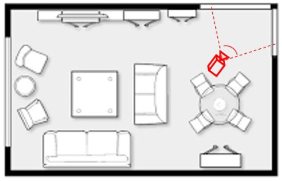
Figure 1.
The performance of a vision-based SLAM is influenced by the field of view.
Another reason for using a full-view camera is that it improves the accuracy of SLAM methods. Because some different motions may have similar changes in an image of a limited FOV camera, these motions are discriminated with a full-view image. For example, as shown in Figure 2, the translation of a limited-view camera along the horizontal axis or rotation in the horizontal direction may result in the same movement for some features on images, i.e., Target 1 in Figure 2. However, for Targets 2–4, the camera motion causes different movements. This means that in some cases, different motions may be difficult to decouple from the observation of limited FOV images, while it is possible to distinguish from the observation of full-view images.
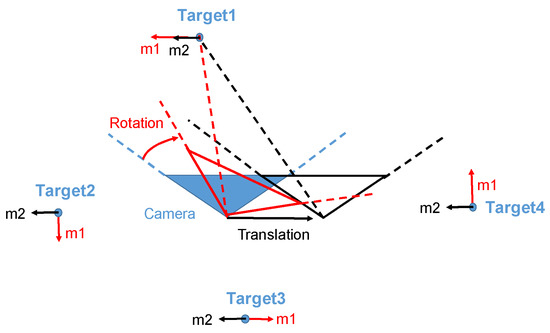
Figure 2.
The translation of a limited-view camera along the horizontal axis and the horizontal rotation may result in the same movement for some features in images (Target 1); however, the same camera motion causes different movements for the features in other places (Target 2–4), only a full-view camera can capture them.
Based on the above observations, a vision-based SLAM method of using full-view images can effectively manage sparse-feature or partially non-feature environments, and also achieve higher accuracy in localization and mapping than conventional limited field-of-view methods. Until now, few SLAM methods for using omnidirectional images have been proposed, and although a wider view results in a better performance in localization and mapping, there are no experiments assessing how accuracy is affected by the view field.
In this paper, we realize simultaneous localization and mapping (SLAM) on full-view images. The principle is similar to the typical approach of the conventional SLAM methods, PTAM (parallel tracking and mapping) [1]. In the proposed method, a full-view image is captured by Ricoh Theta [2]. Next, feature points are extracted from the full-view image. Then, spherical projection is used to compute projection and back-projection of the scene points. Finally, feature matching is performed using a spherical epipolar constraint. The characteristic of this paper is that a spherical model is used throughout processing, from feature extracting to localization and mapping computing.
2. Related Works
In this section, we first introduce the related research in two categories. The first addresses omnidirectional image sensors, while the other addresses the SLAM methods for using omnidirectional image sensors. Then, we explain the characteristics of the proposed method.
2.1. Omnidirectional Image Sensor
A wider FOV means more visual information. One of the methods for covering a wide FOV uses a cluster of cameras. However, multiple camera capture devices are needed, requiring a complicated calibration of multiple cameras. Conversely, it is desirable to observe a wide scene using a single camera during a real-time task. For this purpose, other than fisheye cameras [3], omnidirectional image sensors have been developed, and a popular method uses a mirror combined with a catadioptric omnidirectional camera. The omnidirectional images are acquired using mirrors such as a spherical [4], conical [5], convex hyperbolic [6], or convex parabolic [7]. To acquire a full-view image, a camera with a pair of fisheye lenses was also developed [8].
2.2. Omnidirectional-Vision SLAM
Recently, many vision-based SLAM algorithms have been proposed [9]. According to the FOV of the cameras, these approaches can be grouped into two categories: one is based on perspective images with conventional limited FOV, and the other is an approach that relies on omnidirectional images with hemispherical FOV. Here, we focus the discussion of the related work on those omnidirectional SLAM approaches.
One of the most popular techniques for SLAM with omnidirectional cameras is the extended Kalman filter (EKF). For example, Rituerto et al. [10] integrated the spherical camera model into the EKF-SLAM by linearizing direct and the inverse projection. Developed in [10], Gutierrez et al. [11] introduced a new computation for the descriptor patch for catadioptric omnidirectional cameras that aimed to reach rotation and scale invariance. Then, a new view initialization mechanism was presented for the map building process within the problem of EKF-based visual SLAM [12]. Gamallo et al. [13] proposed a SLAM algorithm (OV-FastSLAM) for omniVision cameras operating with severe occlusions. Chapoulie et al. [14] presented an approach which was applied to SLAM that addressed qualitative loop closure detection using a spherical view. Caruso et al. [15] proposed an extension of LSD-SLAM to a generic omnidirectional camera model. The resulting method was capable of handling central projection systems such as fish-eye and catadioptric cameras.
In the above omnidirectional-vision SLAM, although they used omnidirectional images, their images could still not obtain a view as wide as that of full-view images. Additionally, since processing such as feature extraction and feature matching was not conducted based on the spherical model, they used perspective projection. These approaches are not considered a spherical-model-based approach, according to a recent survey [16].
However, visual odometry and structure from motion are also designed for estimating camera motion and 3D structure in an unknown environment. There are some camera pose estimation methods for full-vision systems were proposed [17]. An extrinsic camera parameter recovery method for a moving omni-directional multi-camera system was proposed; this method is based on using the shape-from-motion and the PnP techniques [18]. Pagani et al. investigated the use of full spherical panoramic images for Structure form Motion algorithms; several error models for solving the pose problem, and the relative pose problem were introduced [19]. Scaramuzza et al. obtained a 3D metric reconstruction of a scene from two highly-distorted omnidirectional images by using image correspondence only [20]. Our spherical model is similar to theirs; their methods also prove that wide-view based on the spherical model has its advantages over limited-view.
The aim of this research is to develop a SLAM method for a mobile robot in indoor environments. The proposed method is based on a spherical model. The problem of tracking failure due to limited view can be completely avoided. Furthermore, as described in Section 1, full-view images also result in better performance for SLAM. The processing of the proposed full-view SLAM method is based on a spherical camera model. The effectiveness of the proposed method is shown using real-world experiments in indoor environments. Additionally, an experiment is also conducted to prove that the accuracy is affected by the view field.
3. Camera Model and Full-View Image
Although the perspective projection model serves as the dominant imaging model in computer vision, there are several factors that make the perspective model far too restrictive. A variety of non-perspective imaging systems have been developed, such as a catadioptric sensor that uses a combination of lenses and mirrors [21], wide-angle lens systems [3], clusters of cameras [22], and a compound camera [23]. No matter what form of imaging system is used, Michael D et al. [24] presented a general imaging model to represent an arbitrary imaging system. In their opinion, an imaging system may be modeled as a set of raxels on a sphere surrounding the imaging system. Strictly speaking, there is not a commercial single viewpoint full-view camera. In this paper, we approximate RICOH-THETA (Ricoh, 2016) as a single viewpoint full-view camera because the distance between the two viewpoint of the fisheye lens of the RICOH-THETA is very small, relative to the observed scenes [25]. This approximation is rather reasonable for a multiple camera motion estimation approach, as mentioned in [26]. The RICOH-THETA camera is only used as a capture device of a single viewpoint full-view image. The captured full-view image is then transformed to a discrete spherical image; the proposed method is based on the discrete spherical image (Figure 3a). The discrete spherical model is referred to [27].
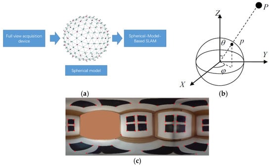
Figure 3.
(a) the proposed method is based on the discrete spherical image; (b)The spherical projection model; (c) full-view image.
Next, we describe the spherical projection model. Suppose there is a sphere with a radius f and a point p in space, as shown in Figure 3b. The intersection of the sphere surface with the line joining point p and the center of the sphere is the projection of the point to the sphere. Suppose the ray direction of the projection is determined by a polar angle, , and an azimuth angle, , and the coordinates of a point p in space is
The projection of point p, in a spherical model, can be represented as
Then, we have the following relation between the two
where .
Let ; we have
This means that m is equal to Mc apart from a scale factor. Let ,
Now we have the normalized spherical coordinate. This corresponds to the projection onto a unit sphere.
Compared with the perspective projection of a planar image based on a pinhole camera model, a full-view image is obtained using the projection of all visible points from the sphere. Thus, a full-view image is the surface of a sphere, with the focus point at the center of the sphere. We use equidistance cylindrical projection to represent a full-view image, as shown in Figure 3c. The corners of squares become more distorted as they approach the poles. Thus, the planar algorithm cannot be applied.
Strictly speaking, the two lenses should be calibrated in a novel calibration process, rather than spherical approximation model, considering that the distance of two viewpoints in RICOH-THETA is smaller than 1 cm, plus, according to the experiments of the absolute errors of the estimated rotation and translation in [26]. Compared to the purely spherical camera, which did not suffer from errors induced by approximation, the spherical approximation had slightly lower performance, but was comparable when the feature tracking error was large. They also showed that the approximation even results in improvements in accuracy and stability of estimated motion over the exact algorithm.
4. Method Overview
Our method continuously builds and maintains a map, which describes the system’s representation of the user’s environment. The map consists of a collection of M point features located in a world coordinate frame W. Each point feature represents a local, spherical-textured patch in the world. The jth point pj on the map has a spherical descriptor dj, and its 3D world coordinate pjW = (xjW, yjW, zjW)T in coordinate frame W.
The map also maintains N keyframes, which are taken in various frame coordinates according to the keyframe insertion strategy. Each keyframe K contains a keyframe index i, the rotation RiK and translation TiK between this frame coordinate and the world coordinate. Each keyframe also stores the frame image IiK, the index of map points ViK, which appear in the keyframe, and the map points’ 2D projection PnViK = (unViK, vnViK)T.
The flow of our full-view SLAM system is shown in Figure 4. Like other SLAM systems, our system also has two main parts: mapping and tracking. The tracking system receives full-view images and maintains an estimation of the camera pose. At every frame, the system performs two-stage coarse-to-fine tracking. After tracking, the system determines whether a keyframe should be added. Once a keyframe is added, a spherical epipolar search is conducted, followed by a spherical match to insert the new map point. The flow of our full-view SLAM system is similar to many existing SLAM approaches. The difference is that these steps are handled based on the spherical model. Each step is now described in detail.
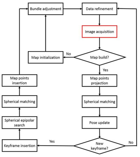
Figure 4.
The flow of our full-view SLAM system.
4.1. Image Acquisition
Images are captured from a Ricoh Theta S and are scaled to 1280 × 640. Before tracking, we run SPHORB, a new fast and robust binary feature detector and descriptor for spherical panoramic images [27]. In contrast to the state-of-the-art spherical features, this approach stems from the geodesic grid, a nearly equal-area hexagonal grid parametrization of the sphere used in climate modeling. It enables us to directly build fine-grained pyramids and construct robust features on the hexagonal spherical grid, avoiding the costly computation of spherical harmonics and their associated bandwidth limitation. The SPHORB feature also achieves scale and rotation invariance. Therefore, each feature point has a specific spherical descriptor.
4.2. Map Initialization
Our system is based on the map. When the system starts, we take two frames, which have a slight offset position between them, to perform the spherical match. Then, we represent feature points using the unit sphere polar coordinate (Equation (5)). Next, we employ the RANSAC five-point stereo algorithm to estimate an essential matrix. Finally, we triangulate the matched feature pair to compute the map point. The resulting map is refined through bundle adjustment [28].
4.3. Map Point Projection and Pose Update
To project map points into the image plane; it is first transformed from the world coordinate to the current frame coordinate C.
where is the jth map point in the current frame coordinate, is the jth map point in the world coordinate, and and represent the current camera pose from the world coordinate.
Then, we project the map point onto the unit sphere, as shown in Equation (5). Then, we detect all the feature points in current frame by SPHORB. Next, we perform a fixed-range search around the unit coordinate . Since the map point has a spherical descriptor, we can compare it with candidate feature points to find the best match point .
Given a pair of matched feature points, and , the angle between the pair of matched feature points can be computed as
Since the spherical point is unit,
Substituting Equations (5) and (6) into Equation (8), we obtain a function about rotation and translation .
Since for a successfully-matched feature point and true rotation and translation , , we can compute rotation and translation by minimizing the following objective function given n matched feature points.
4.4. Two-Stage Coarse-to-Fine Tracking
Because of the distortion of full-view images, even with a slight camera move, the feature point would have a large move on full-view images. To have more resilience when faced with this problem, our tracking system uses the same tracking strategy as PTAM. At every frame, a prior pose estimation is generated from a motion model. Then, map points are project into the image, and their match points are searched at a coarse range. In this procedure, the camera pose is updated based on 50 coarse matches. After this, map points are re-projected into the image. A tight range is used to search the match point. The final frame pose is calculated from all the matched pairs.
4.5. Tracking Recovery
Since the tracking is based on the map point projection, the camera may fail to localize its own position when fewer map points are matched to the current frame. To determine whether the tracking failed, we use a certain threshold of point matching pairs. If the tracking continuously fails for more than a few frames, our system initiates a tracking recovery procedure. We compare the current frame with all keyframes stored on the map using spherical image match. The pose of the closest keyframe is used as the current frame for the next tracking procedure, while the motion model for tracking is not considered for the next frame.
4.6. Keyframe and Map Point Insertion
To maintain our system function, as the camera moves, new keyframes and map points are added to the system to include more information about the environment.
After the tracking procedure, the current frame is reviewed to determine whether it is a qualified keyframe using the following conditions:
- The tracking did not fail at this frame;
- The recovery procedure has not been activated in the past few frames;
- The distance from the nearest keyframe is greater than a minimum distance;
- The time since the last keyframe was added should exceed some frames.
Map point insertion is implemented when a new keyframe is added. First, feature points in the new keyframe are considered as candidate map points. Then, we determine whether the candidate point is near successfully observed map points in the current view. This step helps us to discard candidate points that may already be on the map. Next, we select the closest keyframe by distance since map point insertion is not available from a single keyframe. To establish a correspondence between the two views, we use the spherical epipolar search to limit the search range to a small, but accurate range. Based on the tight search range, spherical matching for the candidate map point is more reliable. If a match has been found, the candidate map point is triangulated. However, until this step, we cannot guarantee the candidate map point is a new point which is not on the map. Therefore, we compare the 3D candidate map point with each existing map point by projecting them onto the first and current keyframe image. If both offsets on the two images are small, we conclude they are the same point, and then connect the current frame information to the existing map point. Finally, the remaining candidate map point is inserted into the map.
4.7. Spherical Epipolar Search
Suppose that the same point is observed by two spherical model cameras. Let the coordinates of the same point at the two camera coordinate systems be and . The pose between the two cameras is represented by a rotation matrix, R, and a translation vector, T. According to the coplanar principle, we have
where and
By using the spherical projection in Equation (4), we have
Given m1 is known, according to Equation (5), we represent Equation (12) as
where
In practice, we give an error range
Equation (15) gives the constraint for the spherical epipolar search and identifies the corresponding feature point.
4.8. Data Refinement
After a new keyframe and new map points are added, bundle adjustment must be used as the last step. In our map, each map point corresponds to at least one keyframe. Using keyframe pose and 2D/3D point correspondences, each map point projection has an associated reprojection error, calculated as Equation (7). Finally, bundle adjustment iteratively adjusts all map points and keyframes to minimize the error.
The added map point may be incorrect because of matching error. To distinguish the outliers, for every frame tracking, we calculate the reprojection error of visible map points in the current frame. If the number of map point errors exceeds the number of correct map points, the map point is discarded.
5. Validation
The system described above was implemented on a desktop PC with a 2.5 GHz Intel(R) CoreTM i5-2400S processor and 8 GB RAM. To evaluate the performance of our full-view SLAM system, we first evaluated our system in a small workspace to test system functions. Then, we used an accuracy test on a measured route, which was in a sparse feature environment. Last, we moved the camera in a room to conduct a real-world test. As this paper focuses on emphasizing the advantage of the full-view-based method over limited-view-based methods, we conducted an experiment to show that the accuracy decreased while the field of view decreased.
5.1. Functions Test
We prepared a video with 2429 frames. This video, which was recorded from a full-view model camera, explored a desk and its immediate surroundings. First, we let the camera move in front of the desk to produce an overview of the scene. Then, the camera moved away from the desk. Next, we occluded the camera and let it try to recover tracking at a place near the desk. The full test video can be seen at https://youtu.be/_4CFIPA5kZU.
The final map consisted of 31 keyframes and 1243 map points. We selected nine frames (frame index: 134, 356, 550, 744, 1067, 1301, 1639, 1990, and 2103) from the test video to illustrate the performance, as shown in Figure 5. The yellow plane in these figures represents the world coordinate system, which was established using map initialization. The yellow plane was stable in the environment during this test. Whether the camera was far or near to an object, our system functioned well. The final map is shown in Figure 6. From the map, we identified the laptop PC, desktop PC, and other items. We also tested the tracking recovery, which was very important to camera re-localization, in this video. It was also used to evaluate our tracking and mapping system. We occluded the camera at frame 2171 and stopped occluding at frame 2246. Simultaneous with the occluding, we moved the camera from a distant place to a closer place relative to the desk. Our system successfully localized itself after being moved (Figure 7).
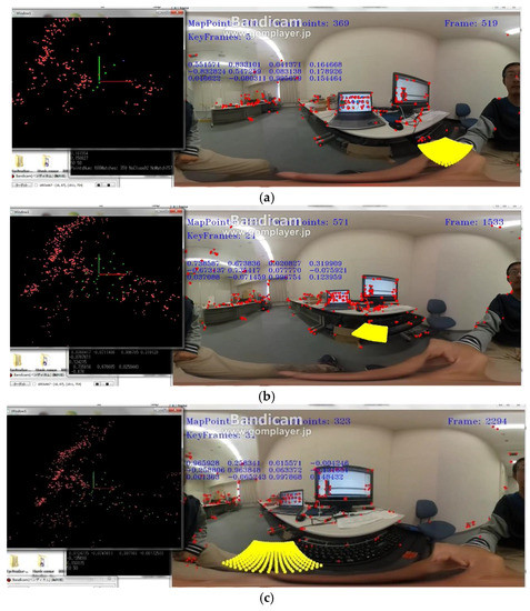
Figure 5.
Sample frames from the desk video. (a) Frame 519; (b) Frame 1533; (c) Frame 2294.
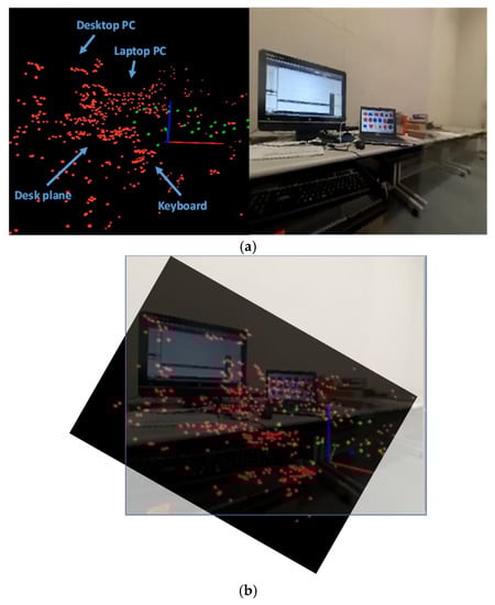
Figure 6.
The map produced in the desk video. (a) map points and its corresponding real situation; (b) the map points are coincide with the real situation.
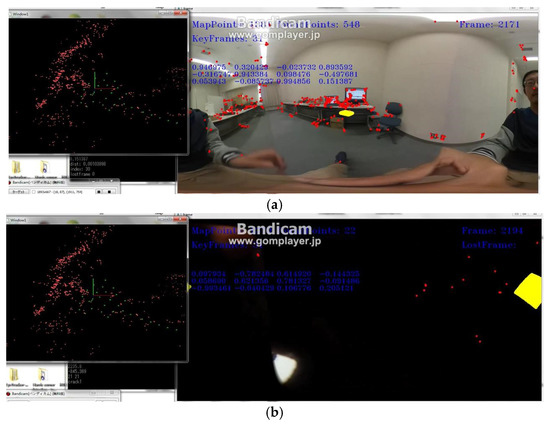
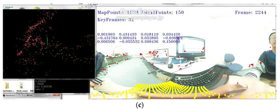
Figure 7.
Tracking recovery in the desk video. (a) Tracking well before occlusion; (b) Let the system lost tracking; (c) Tracking recovery even the location is changed.
5.2. Accuracy Test
To validate our system further and compare with the limited-view method (PTAM), we measured routes in a space with sparse features, as shown in Figure 8. The camera moved from the starting point to the ending point with no rotation as quickly as possible. The first 10 cm was used for map initialization; we provided the real scale for the system. During the test, the limited-view SLAM failed because the environment was sparse. Only a few features were captured in limited views. We tested PTAM [1], one of the most famous limited-view SLAM approaches, on perspective images generated directly from full-view images. Figure 9 shows that PTAM failed to track in a sparse feature environment, which was a wall in this test. However, our full-view SLAM tracked well in this situation because it can capture features from other place except the wall. The final map is shown as the left image in Figure 10. Two boxes were defined in the final map. The coordinate system on the map was the world coordinate system, which was also the starting point in this test. Each green point represents a keyframe. The trajectory, which was very close to the ground truth, is shown as the right image in Figure 10. The video can be seen at https://youtu.be/c1ER1OqyjXM.
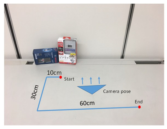
Figure 8.
A measured route in a sparse environment.
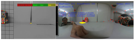
Figure 9.
At the same position, PTAM fails to track as fewer feature points visible, while full-view SLAM tracks well.
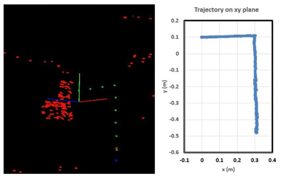
Figure 10.
The map and the trajectory for Figure 9.
Then, we conducted an experiment to test our system’s accuracy in a larger environment. We planned a new, measured route, as shown in Figure 11. The camera moved in a clockwise loop through 16 marked points, we randomly put a few objects around the route to generate a sparse space, plus, no objects are put around points 9–12. Point A was the starting point. The first 10 cm from A to B was used for map initialization. Using continuous tracking and mapping, we obtained the distance between point A and every marked point. We measured the ground truth using a laser rangefinder. The final errors for every marked point using our method are shown in Table 1 and Figure 12. As seen in Table 1, the accuracy of marked points (8–12) decreased compared to the other points. The reason is that we set few trackable features around these marked points to simulate a sparse environment. Our proposed method is based on full-view images. It uses the features from every direction, so this had only a small influence on our system. However, limited-view based methods, such as PTAM [1], immediately failed to track at these points because of a limited view with few features. The result shows that our method tracked in a sparse environment, and that the accuracy of our method was sufficient. The average error was 0.02 m.
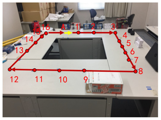
Figure 11.
The designed route.

Table 1.
The accuracy compared with ground truth.
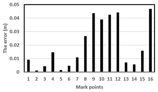
Figure 12.
The errors of marked points.
5.3. Route Test
In this section, we demonstrate the performance of our system in real-world situations. We allowed the camera to move along the wall in a square in a room to build the map. Some sample frames are shown in Figure 13 to illustrate the formation of the map and the trajectory. We marked “P” on map images to define the current camera positions and marked “door” on both the full-view image and map image. Readers may find the relationship between the map and the real environment easier to understand using these markers. The final trajectory was a square as planned. The video is available at https://youtu.be/QzilX069U0M. The surrounding estimation and the trajectory were similar to that of the real environment.

Figure 13.
Sample frames from the indoor test.
To have a further validation on route test, as Figure 14a shows, we put the full-view camera on the MAV, then let the MAV fly on a planned route. One side of the route is a tall building with unique features, while the other side is full of trees with confusing features. The final trajectory is very close to our planned route. Our final estimated trajectory, the trajectory from PTAM, and the trajectory from GPS, are compared in Figure 14. PTAM performs badly and even loses tracking as MAV rotates, because limited-view SLAM systems would not insert the keyframe if only rotation happens. And the trajectories from our system and GPS are very close, but around the start point, the GPS has some errors, which is more than the estimated trajectory by our system. The GPS trajectory shows that the MAV is very close to the wall, which is not possible; this is because the GPS signal may be affected by the tall building nearby. The whole test video by our system is available on https://youtu.be/R8C_W5HY1Dg.
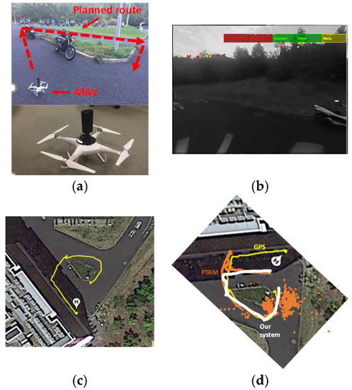
Figure 14.
(a) full-view camera on the MAV; (b)PTAM performs badly as MAV rotates or in a sparse feature view; (c) GPS flight trajectory; (d) The flight trajectory by GPS, PTAM, and our system.
5.4. Accuracy Validation with a Decrease in the Field of View
In this section, we validate the inherent disadvantages of limited-view based methods. We discuss the decreased field of vision and how the performance of our system would behave. Similar to Section 5.2, we designed a route and collected full-view images for tracking and mapping. To decrease the field of view from full-view images, we decreased the range of theta since the full-view image was presented in the spherical model (Figure 15). Thus, we obtained limited-view images with desirable view angles. We tested our system with (theta = 160, 140, 120, 100, 80 degrees) views, and the experiment was conducted ten times. Each time, the limited-view was generated randomly, so the tracking result was different depending on the features. The accuracy with different theta values is listed in Table 2.
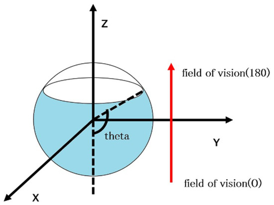
Figure 15.
Achieving limited view from full-view images by decreasing theta.
Table 2.
The accuracy with different theta.
As shown in Table 2, as the field of view decreased, the accuracy decreased. When the field of view was less than 100 degrees, some experiments failed to track (‘X’ in Table 2). Because a limited view means limited information, only limited features from one direction could not retrain a result as accurately as from all directions, especially for sparse environments. The average error showed that wider views resulted in a better performance.
6. Conclusions
In this paper, we presented a full-view SLAM system for full-view images. Based on the spherical model, our system allowed tracking features even in a sparse environment. However, the limited-view SLAM systems did not perform well. The contribution of this paper is that we realized tracking and mapping directly on full-view images. Key algorithms of SLAM were all adjusted to a spherical model.
The experiment showed that our method could successfully be applied in camera pose estimation in an unknown scene. Since our system was recently developed, no processing optimization was considered, and we did not validate the time cost in this paper. Future works will consider increasing the speed of our system using multi-threads and GPU.
Author Contributions
Software, J.L.; Supervision, S.L.; Validation, J.L. and X.W.; Writing—original draft, J.L.; Writing—review & editing, S.L.
Funding
This work is supported by Fundamental Research Funds for the Central Universities (SWU20710916).
Conflicts of Interest
The authors declare no conflict of interest.
References
- Klein, G.; Murray, D. Parallel tracking and mapping for small AR workspaces. In Proceedings of the 6th IEEE/ACM ISMAR, Nara, Japan, 13–16 November 2007; pp. 225–234. [Google Scholar]
- Available online: https://theta360.com/en/ (accessed on 1 October 2018).
- Miyamoto, K. Fish eye lens. J. Opt. Soc. Am. 1964, 54, 1060–1061. [Google Scholar] [CrossRef]
- Hong, J.; Tan, X.; Pinette, B.; Weiss, R.; Riseman, E.M. Image-based Homing. In Proceedings of the 1991 IEEE International Conference on Robotics Automation, Sacramento, CA, USA, 9–11 April 1991; pp. 620–625. [Google Scholar]
- Yagi, Y.; Kawato, S.; Tsuji, S. Real-time omni-directional vision for robot navigation. Trans. Robot. Autom. 1994, 10, 11–22. [Google Scholar] [CrossRef]
- Yamazawa, K.; Yagi, Y.; Yachida, M. Omnidirectional imaging with hyperboloidal projection. In Proceedings of the 1993 IEEE/RSJ International Conference on Intelligent Robots and Systems, Yokohama, Japan, 26–30 July 1993; pp. 1029–1034. [Google Scholar]
- Nayar, S.K. Catadioptric omnidirectional camera. In Proceedings of the IEEE Computer Society Conference on Computer Vision and Pattern Recognition, San Juan, PR, USA, 17–19 June 1997; pp. 482–488. [Google Scholar]
- Li, S. Full-view spherical image camera. In Proceedings of the 18th International Conference on Pattern Recognition (ICPR’06), Hong Kong, China, 20–24 August 2006; pp. 386–390. [Google Scholar]
- Fuentes-Pacheco, J.; Ruiz-Ascencio, J.; Rendon-Mancha, J. Visual simultaneous localization and mapping: A survey. Artif. Intell. Rev. 2015, 43, 55–81. [Google Scholar] [CrossRef]
- Rituerto, A.; Puig, L.; Guerrero, J.J. Visual SLAM with an omnidirectional camera. In Proceedings of the 20th International Conference on Pattern Recognition, Istanbul, Turkey, 23–26 August 2010; pp. 348–351. [Google Scholar]
- Gutierrez, D.; Rituerto, A.; Montiel, J.M.M.; Guerrero, J.J. Adapting a real-time monocular visual SLAM from conventional to omnidirectional cameras. In Proceedings of the IEEE International Conference on Computer Vision Workshops (ICCV Workshops), Barcelona, Spain, 6–13 November 2011; pp. 343–350. [Google Scholar]
- Valiente, D.; Jadidi, M.G.; Miró, J.V.; Gil, A.; Reinoso, O. Information-based view initialization in visual SLAM with a single omnidirectional camera. Robot. Auton. Syst. 2015, 72, 93–104. [Google Scholar] [CrossRef]
- Gamallo, C.; Mucientes, M.; Regueiro, C.V. Omnidirectional visual SLAM under severe occlusions. Robot. Auton. Syst. 2015, 65, 76–87. [Google Scholar] [CrossRef]
- Chapoulie, A.; Rives, P.; Filliat, D. A spherical representation for efficient visual loop closing. In Proceedings of the IEEE International Conference on Computer Vision Workshops (ICCV Workshops), Barcelona, Spain, 6–13 November 2011; pp. 335–342. [Google Scholar]
- Caruso, D.; Engel, J.; Cremers, D. Large-scale direct SLAM for omnidirectional cameras. In Proceedings of the IEEE/RSJ International Conference on Intelligent Robots Syst. (IROS), Hamburg, Germany, 28 September–2 October 2015; pp. 141–148. [Google Scholar]
- Taketomi, T.; Uchiyama, H.; Ikeda, S. Visual SLAM algorithms: A survey from 2010 to 2016. IPSJ Trans. Comput. Vis. Appl. 2017, 9, 16. [Google Scholar] [CrossRef]
- Scaramuzza, D.; Fraundorfer, F. Visual Odometry [Tutorial]. Robot. Autom. Mag. 2011, 18, 80–92. [Google Scholar] [CrossRef]
- Sato, T.; Ikeda, S.; Yokoya, N. Extrinsic Camera Parameter Recovery from Multiple Image Sequences Captured by an Omni-Directional Multi-camera System. In Proceedings of the European Conference on Computer Vision, Prague, Czech Republic, 11–14 May 2004; Volume 2, pp. 326–340. [Google Scholar]
- Pagani, A.; Stricker, D. Structure from Motion using full spherical panoramic cameras. In Proceedings of the IEEE International Conference on Computer Vision Workshops IEEE, Barcelona, Spain, 6–13 November 2011; pp. 375–382. [Google Scholar]
- Scaramuzza, D.; Martinelli, A.; Siegwart, R. A Flexible Technique for Accurate Omnidirectional Camera Calibration and Structure from Motion. In Proceedings of the IEEE International Conference on Computer Vision Systems IEEE, New York, NY, USA, 4–7 January 2006; p. 45. [Google Scholar]
- Nayar, S.K.; Baker, S. Catadioptric image formation. In Proceedings of the Darpa Image Understanding Workshop, Bombay, India, 1–4 January 1998; Volume 35, pp. 35–42. [Google Scholar]
- Swaminathan, R.; Nayar, S.K. Nonmetric Calibration of Wide-Angle Lenses and Polycameras. IEEE Trans. Pattern Anal. Mach. Intell. 2000, 22, 1172–1178. [Google Scholar] [CrossRef]
- Gaten, E. Geometrical optics of a galatheid compound eye. J. Comp. Physiol. A 1994, 175, 749–759. [Google Scholar] [CrossRef]
- Grossberg, M.D.; Nayar, S.K. A General Imaging Model and a Method for Finding its Parameters. Computer Vision. In Proceedings of the Eighth IEEE International Conference on Computer Vision, Vancouver, BC, Canada, 7–14 July 2001; Volume 2, pp. 108–115. [Google Scholar]
- Available online: https://theta360.com/en/about/theta/technology.html (accessed on 1 October 2018).
- Kim, J.S.; Hwangbo, M.; Kanade, T. Spherical Approximation for Multiple Cameras in Motion Estimation: Its Applicability and Advantages. Comput. Vis. Image Underst. 2010, 114, 1068–1083. [Google Scholar] [CrossRef]
- Zhao, Q.; Feng, W.; Wan, L.; Zhang, J. SPHORB: A fast and robust binary feature on the sphere. Int. J. Comput. Vis. 2015, 113, 143–159. [Google Scholar] [CrossRef]
- Triggs, B. Bundle adjustment—A modern synthesis. In International Workshop on Vision Algorithms; Springer: Berlin/Heidelberg, Germany, 1999; pp. 298–372. [Google Scholar]
© 2018 by the authors. Licensee MDPI, Basel, Switzerland. This article is an open access article distributed under the terms and conditions of the Creative Commons Attribution (CC BY) license (http://creativecommons.org/licenses/by/4.0/).