Article

Analysis of Lightweight Feature Vectors for Attack Detection in Network Traffic

Institute of Telecommunications, TU Wien, 1040 Wien, Austria
*
Author to whom correspondence should be addressed.
Appl. Sci. 2018, 8(11), 2196; https://doi.org/10.3390/app8112196
Submission received: 25 October 2018 / Revised: 5 November 2018 / Accepted: 6 November 2018 / Published: 9 November 2018

Abstract

:

Featured Application

Optimal design of feature vectors for early-phase attack detection in large communication networks.

Abstract

The consolidation of encryption and big data in network communications have made deep packet inspection no longer feasible in large networks. Early attack detection requires feature vectors which are easy to extract, process, and analyze, allowing their generation also from encrypted traffic. So far, experts have selected features based on their intuition, previous research, or acritically assuming standards, but there is no general agreement about the features to use for attack detection in a broad scope. We compared five lightweight feature sets that have been proposed in the scientific literature for the last few years, and evaluated them with supervised machine learning. For our experiments, we use the UNSW-NB15 dataset, recently published as a new benchmark for network security. Results showed three remarkable findings: (1) Analysis based on source behavior instead of classic flow profiles is more effective for attack detection; (2) meta-studies on past research can be used to establish satisfactory benchmarks; and (3) features based on packet length are clearly determinant for capturing malicious activity. Our research showed that vectors currently used for attack detection are oversized, their accuracy and speed can be improved, and are to be adapted for dealing with encrypted traffic.

1. Introduction

The omnipresence of network communications—whether we refer to individual persons, societies, companies, or governments—emphasizes the importance of understanding network traffic shapes and properties. The application of network traffic monitoring and analysis are fundamentally intended to enhance security, but also the quality of services and the design of infrastructures and devices. Additionally, scientific research makes the most of network traffic analysis in areas related to telecommunications engineering, data science, and machine learning, among others.
From an analytic perspective, network traffic shows some characteristics that strongly challenge analysis frameworks. For instance, network traffic involves: Large datasets, continuous generation of data, high variability and fast evolution of shapes and classes, encrypted information, time-dependency, malicious traffic designed to bypass detection, and the necessity of triggering prompt reactions (mainly for security purposes). Given such a challenging scenario, selecting suitable traffic representations is a relevant and delicate issue. Even with the best analysis algorithms and frameworks, a wrong selection of features will inevitably lead to failure. A second relevant aspect—frequently forgotten in the related research—is that effective attack detection in real environments must be faced by combining multiple techniques in different phases [1]. In keeping with this design idea, first-phase traffic detectors—the ones addressed here—act as filters that classify and discriminate a major proportion of traffic, therefore allowing more complex algorithms to focus on a small part of the incoming data for an in-depth analysis.
Regardless of the desired level of the analysis depth, the possibilities to extract features from network traffic captures are immense. However, extracting large vectors from traffic should be avoided. Working with compact, highly relevant feature sets is recommended, as it leads to better results. This is not a particular rule for network traffic, but a general recommendation in data analysis. As emphasized by Guyon and Elisseeff [2], a good feature selection (1) improves analysis performances, (2) speeds up the analysis process, and (3) helps to understand the underlying mechanisms that generated the data. On the other hand, the field of network traffic implies additional limitations to take into account when designing feature vectors; two of the most outstanding are: Data encryption and the overgrowing increase of data generated in networks (i.e., big data) [1]. These two factors have made deep packet inspection infeasible and inefficient. Instead, modern traffic analysis techniques rely on analyzing footprints and profiles obtained from flow-features, which are extracted from packet headers and communication characteristics that do not require checking packet contents [3].
However, as discussed by Ferreira et al. [4], there are no clear, standard methodologies for analyzing network traffic or general recommendations that suggest a specific set of features, except for cases in which a very well-defined traffic class is aimed. Experts simply follow their intuition and field experience, perhaps resort to previously published works, or acritically apply models and tools with default configurations. In short, the selection of features for attack detection in network security is an open discussion.
In this work, we studied five feature sets (we indistinctly use feature vector and feature set throughout the paper) that have been proposed in the scientific literature for the last few years. The selected vectors are equally devised for the fast analysis of traffic in large networks, meaning that they are able to perform traffic classification, discriminate malware from normal traffic, and detect anomalies. Moreover, they are based on flow features and are suitable for encrypted data and big data analysis. We compared and evaluated them in terms of classification performance and computational costs. Additionally, we analyzed the importance of individual features for the classification accuracy. For our experiments, we used the UNSW-NB15 dataset, which consists of 100 GB of labeled traffic and contains legitimate, normal communications mixed with attacks and anomalies that belong to nine different families of malicious activities. This dataset was published in 2015 to become a replacement for the old, widely used KDD dataset family.
Results showed that the most effective feature set in terms of classification performance is based on modeling the behavior of sources instead of separately checking communication flows (note that, in the given context, sources are meant to be any network device that sends and receives traffic, either servers, clients or routers. For such sources, only the sending activity is profiled, vectorized, and analyzed). On the other hand, a feature set designed from a consensus of the most important field research for the last few years obtains good trade-offs between classification and computational costs. Finally, the analysis of features shows that calculations based on packet lengths are determining for classifying traffic and detecting attacks, followed—but with lower relevance—by calculations based on the use of TTLs (Time to Live), number of packets, and number of bytes. The conducted experiments and the observed results are useful to face the design of improved feature vectors for applications related to both network security and network traffic analysis.
The rest of the paper is organized as follows: Section 2 describes the studied feature vectors, Section 3 presents the dataset used for evaluation, Section 4 explains the conducted experiments, Section 5 shows and discusses results, Section 6 faces results from the perspective of data encryption, and Section 7 summarizes findings and concludes the work.

2. Feature Sets

In this section, we introduce the problem of extracting features from encrypted traffic and describe the feature vectors under study. Feature vectors are shown together in Table 1. For the sake of clarity and to allow better comparisons, some feature names have been modified when contrasted with the original sources; for instance, “srcIP”, “srcip”, “sourceIP”, and “sourceIPv4Address” refer to the same feature and are here expressed as “srcIP”. We have modified the names of most common features, trying to keep self-explanatory terms. In case of doubt, we refer the interested reader to the original sources for complete feature descriptions and original names (original sources are provided in the respective subsection of Section 2 corresponding to every studied feature set).

2.1. UNSW-NB15 Argus/Bro Feature Vector

The UNSW-NB15 Argus/Bro vector is the analysis format chosen by the authors who published the dataset used in the experiments. The dataset itself is introduced later in Section 3. Moustafa and Slay [5,6] extracted features from raw pcaps with Argus https://qosient.com/argus/ and Bro https://www.bro.org/, which are popular tools for network security and have been widely used in research for many years [7,8]. The meaning and description of features are provided in the referred works [5,6], and we show them here in Table 1. We keep this feature vector for our analysis since: (1) It is the one proposed by dataset authors, (2) features are extracted with such popular network security tools, and (3) this vector is being used by other security experts that also use the UNSW-NB15 dataset for their research, e.g., the authors of [9].
The UNSW-NB15 Argus/Bro vector consists of 45 predictors (i.e., features used to guess the sample class), and mixes nominal, numerical, and binary features. For our experiments, we used the preprocessed dataset provided by the authors. Figure 1 shows some scatter plots of randomly selected UNSW-NB15 numerical features.

2.2. CAIA Feature Vector

The name of “CAIA” is taken from the Centre for Advanced Internet Architectures at the Swinburne University of Technology (http://www.caia.swinburne.edu.au/), which is the research group and institution hosting the authors that first used this vector to the best of our knowledge. In their paper, Williams et al. [10] compared different machine learning techniques for performing traffic flow classification. Since then [10], the same features have often been used with minimal modifications in some relevant, frequently cited works related to flow-based traffic analysis with machine learning. For example, almost the same set is applied by Lim et al. [11], who investigate why some features are so decisive for machine learning algorithms. The same feature vector was recently used by Vlădut̨u et al. [12]. Additionally, Zhang et al. [13]—yet not specifically referring to the previous works—used the same feature set, but in a unidirectional fashion. Anderson and McGrew [14] refer to the CAIA feature set as a ground benchmark for their experiments with encrypted traffic.
The CAIA vector is originally presented in Reference [10] with 22 features that collect bidirectional information. We added 8 features related to TCP (Transmission Control Protocol) flags following the use in Reference [11]. Therefore, the final vector is formed by 30 features (Table 1).

2.3. Consensus Feature Vector

Ferreira et al. [4] address the problem of selecting features for traffic classification and anomaly detection from a meta-analysis perspective. In their work, they selected 71 related papers according to relevance and publication quality criteria and studied the features applied for the analysis. Using metrics based on number of appearances and number of paper citations, the work concluded in a set of 12 features that significantly stand out over the rest of features used in the examined papers. Two such features are “server_to_client”, and “client_to_server”, which mark the bidirectional character of a possible Consensus vector. Essentially, this fact means that in the scope of our analysis, some features must be duplicated to show the direction of the flow; for instance, “pkts” transforms into “srcPkts” and “dstPkts”. Additionally, Ferreira et al. [4] inform that some of the outstanding features are submitted to different operations (e.g., mean, logarithm, sum) depending on the consulted paper. Taking all these factors into account, we built the final Consensus vector as shown in Table 1, which is formed by 19 features.

2.4. Time–Activity Feature Vector

The Time–Activity vector is proposed by Iglesias and Zseby [15] to explore fast normal IP communications by means of unsupervised methods. It is a simple and straightforward feature set that captures the time-behaviour of flows, unidirectionally, with a one-second time resolution, and in a one-minute time scope. This method observes flows from a time series perspective and creates a vector using key numerical values that explain the time-behavioral profile. The final vector—considering also srcPort, dstPort and protocol—is formed by 13 features (Table 1). In Reference [15], nominal features are not used for the analysis, but in the preprocessing (splitting data into datasets) and, later, for the manual evaluation of results.

2.5. AGM Feature Vector

The AGM (AGgregation & Mode) vector was originally proposed for the exploration and discovery of patterns in the Internet Background Radiation [16]. Defined for unidirectional traffic, this vector captures the behavior of hosts by observing the use of eight lightweight flow features, plus the total number of packets. Features are: srcIP, destIP, srcPort, dstPort, Protocol, TCPflag, TTL, and pktLength. After selecting how hosts are profiled—either as data-senders (sources) or data-receivers (destinations)—and an observation time, the basic AGM vector stores the number of unique values, the mode, and the number of packets assigned to the mode of every one of the previous features (for instance, “dstPort” becomes “#dstPort”, “mode_dstPort”, and “pkts_mode_dstPort”). Thus, the basic AGM vector contains 22 features ( 7 × 3 + total number of packets; see Table 1). To operate solely with numerical features, the extended AGM vector removes some nominal features that show a highly spread distribution (e.g., mode_dstIP) or transforms them into a set of dummy variables (aka one-hot encoding) based on expected values shown in frequency tables (e.g., “mode_protocol” transforms into the binary “TCP”, “UDP”, and “ICMP” features, and other possible protocols get 0 for these tree new features). The AGM traffic representation can be further consulted in Reference [16].

3. The UNSW-NB15 Dataset

The lack of labeled TCP/IP data for research and algorithm testing is a classic problem in network security. The KDD family (KDD Cup’98, KDD Cup’99 and NSL-KDD) is formed by perhaps the most popular datasets in this regard. They have been widely used for the last 20 years, in spite of the received criticisms. Tavallaee et al. [17] proposes the NSL-KDD dataset to partially overcome the defects of the previous versions, yet it is still based on the same old captures. The KDD family is therefore severely outdated and, 20 years later, hardly represents current communications and attacks.
More recently, Moustafa and Slay [5,6] presented the UNSW-NB15 dataset to be “a new benchmark dataset for evaluating NIDSs”. The UNSW-NB15 is formed by legitimate traffic and attacks split into nine different big categories: Fuzzers, analysis, backdoors, DoS, exploits, generic, reconnaissance, shellcode, and worms. Datasets are provided in raw captures (pcaps, 100 GB) supported by a ground truth CSV file, as well as already preprocessed and separated into training and test datasets in the Argus-Bro format. In terms of flows, the UNSW-NB15 total figures are shown in Table 2.
Traffic data for this dataset were originally generated by an IXIA PerfectStorm platform: A powerful commercial solution designed to simulate large networks and evaluate security aspects (http://www.ixiacom.com/products/perfectstorm). The tool generated 100 GB of both legitimate communications and attacks, collected in two simulated periods: 16 h corresponding to 22 January 2015 and 16 h for 17 February 2015. We joined both periods in our experiments. For the attack generation, the platform obtained information related to novel malware from a CVE (Common Vulnerabilities and Exposures (CVE)) site, which is continuously updated (https://cve.mitre.org/). In the cited papers, Moustafa and Slay [5,6] developed a deep study about the statistical and practical suitability of the dataset by itself and when compared with its predecessors. The UNSW-NB15 dataset is publicly available and can be downloaded from the authors’ website (https://www.unsw.adfa.edu.au/australian-centre-for-cyber-security/cybersecurity/ADFA-NB15-Datasets/).

4. Experiments

In this section, we explain the experimental methodology that we followed to compare feature sets. We also introduce the applied classification schemes and the different evaluation metrics. The scheme in Figure 2 summarizes the experiments. The used software consisted of a flow-extractor tool developed in Golang (https://golang.org/) and Python scripts for the framework and analysis tasks, which used the scikit-learn (http://scikit-learn.org/stable/), pandas (https://pandas.pydata.org/) and numpy (http://www.numpy.org/) libraries. The used scripts are publicly available for experiment repeatability from our website in Reference [18].

4.1. Experimental Prerequisites

  • A TCP/IP dataset containing normal traffic and attacks (Section 3). This dataset is available as raw captures (pcaps) and already preprocessed in a CSV file according to the UNSW-NB15 Argus/Bro format (Section 2.1).
  • A Ground Truth (GT) file with information linking attacks and flows in the dataset, provided together with the UNSW-NB15 dataset (Section 3).
  • Five sets of feature vectors to represent traffic (introduced in Section 2).

4.2. Experimental Design and Setup
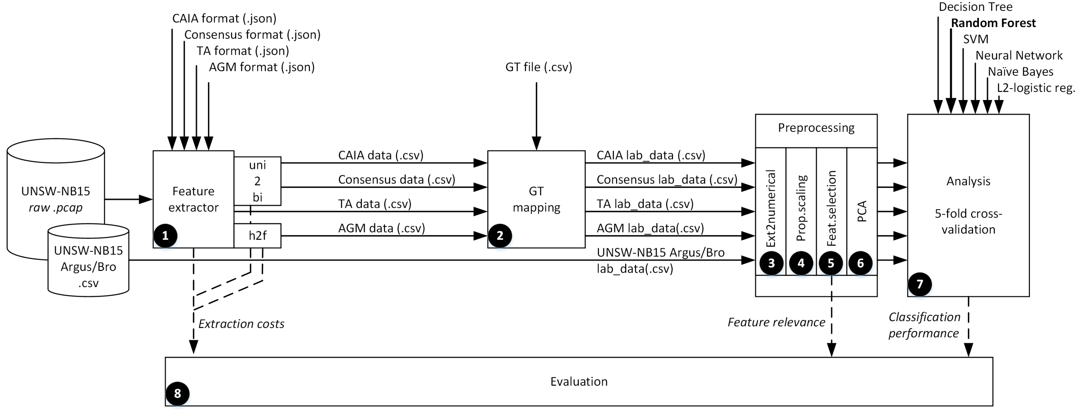
Step-by-step experiments were (scheme in Figure 2):
  • Basic Feature Extraction
    Features were obtained from pcaps with a feature extractor developed in Golang. The process was the same for the CAIA, Consensus, Time–Activity (TA), and AGM vectors. As for the UNSW-NB15 Argus/Bro case, we directly used the published preprocessed data. The UNSW-NB15 Argus/Bro requires the use of Argus and Bro tools, in addition to 12 models that have not been published in the consulted sources. Due to the fact that the UNSW-NB15 format consists of a higher number of features (also more costly to extract) than the other vectors, we assumed that the UNSW-NB15 Argus/Bro vector is one of the most resource-demanding vectors for the extraction-cost comparison. Another special case is the AGM format, which requires a specific aggregation-step to transform the 8 basic features into the defined AGM vector with 22 features.
    In order to allow a fair comparison, CAIA and Consensus vectors, which are bidirectional defined, underwent an additional phase to convert unidirectional vectors into bidirectional vectors (uni2bi). Finally, the AGM format, which addresses source-behavior instead of flow-behavior (in the context of this work, a “flow” is defined by the classic 5-tuple format: srcIP, dstIP, srcPort, dstPort and protocol), required a conversion to unfold its samples and match the flow-key used by the other four vectors (h2f).
  • GT Mapping
    Extracted data in the different formats were cross-checked with the GT file to assign the corresponding labels to training and test datasets. There are two types of labels: Binary (0-legitimate, 1-attack) and multiclass (identifying the nine attack families contained in the used dataset). In this step, all flows were initially labeled as "legitimate" (i.e., 0-label), and later labels were overwritten whenever processed flows appeared in the GT file. The mapping script used flow-keys and timestamps to find the correct matching between flows and threats. The corresponding statistics are in Table 2.
  • Extension to Numerical Vectors
    In order to analyze data with purely numerical classification schemes, nominal variables were transformed into dummy variables [19]. To avoid the generation of high-dimensional sparse spaces, we used the method proposed in Reference [16], which explores the distribution of training data with frequency tables and creates variables accordingly. We also intentionally removed srcPort and dstPort from analyzed vectors to dissociate our experiments from port-based analysis. In any case, srcPort and dstPort showed low relevance or were directly negligible during preliminary experiments for all vectors. This fact does not necessarily mean that these features are not useful for discriminating traffic attacks; instead, they must be considered of low importance in the context of every vector, which might contain more revealing features highly correlated with port information (srcPort is usually irrelevant also from a general perspective). Removing srcPort and dstPort is also a good initiative from a perspective of analyzing encrypted traffic (see discussions in Section 6 and Section 6.1). Table 3 shows the new binary variables created based on frequency tables.
  • Proportional Scaling
    We normalized features in training and test datasets according to training max and min values. We preferred proportional scaling before standardization to avoid the manipulation of original feature variances.
  • Feature Selection
    We carried out feature selection with decision trees for every feature vector. Afterwards, we removed irrelevant features (importance = 0, labeled as “negligible” in Table 6). Additionally, we analyzed the most relevant features for each case. The scheme used for feature selection is a linear decision tree implemented in Python with the scikit-learn library tools (scikit-learn v0.19.1, [20], http://scikit-learn.org/.../sklearn.tree.DecisionTreeClassifier.html). Decision tree maximum depth and minimum leaf size were adjusted by means of a randomized parameter search in order to optimize the performance and avoid overfitting (http://scikit-learn.org/stable/modules/generated/sklearn.modelselection.RandomizedSearchCV.html).
  • PCA-Based Transformation and Reduction
    To facilitate algorithm operations and work with a further reduced feature set, we applied PCA (Principal Component Analysis) as a last step of the preprocessing. PCA is a way to minimize feature dependencies, simplify learning models, and optimize classification performance [21]. First, training means were removed from training and test data to eliminate the intercept. This step is required when applying PCA to guarantee accurate approximations and reduce the mean square error [22]. Second, training and test data were projected based on training data PCA coefficients. Last, feature selection was applied again to remove final irrelevant features (if any) from the new problem space and reduce the dimensions of the resulting vector from PCA. This second feature selection step was also driven by the GT-labels (external criteria) to avoid losing information about classes that show low representativity in the training data.
  • Cross-Validated Supervised Classification
    Applied algorithms were all based on models and operated on training and test datasets following a 5-fold cross-validated evaluation. All algorithms were also implemented in Python with the scikit-learn library (scikit-learn v0.19.1, [20]). Since some parameters showed a considerable sensitivity and broad ranges, the parameterization of learners was adjusted by means of evolutionary search (https://github.com/rsteca/sklearn-deap). The used algorithms were:
    Preliminary experiments with all feature vectors showed the best performances (in all cases) for random forests, followed by decision trees. Naive Bayes classifiers and logistic regression obtained the worst performances, which was expected for the case of the Bayes classifier due to the high correlation commonly shown by network traffic features [23]. Random forests and decision trees not only outperformed other learners, but they were also the most robust ones. Neural networks and support vector machines obtained lower performances than random forests as well as nondeterministic issues, meaning that they suffered noticeable performance drifts in different runs with the same parameters. As a general rule, all learners in their best performances show the same preferences among the studied vectors. Due to these reasons and for the sake of simplicity, in Section 5, we only show classification results obtained with random forests. We address the interested readers to examine the complete experiments available in Reference [18].
  • Evaluation
    The evaluation considered three different perspectives:
    (a)
    Comparison of classification performances using common metrics in supervised classification: Accuracy, precision, recall, f1-scores, and AUC/ROC (http://scikit-learn.org/.../classes.html#module-sklearn.metrics);
    (b)
    Comparison of feature extraction costs for every different feature vector;
    (c)
    Scoring feature importances in every feature vector based on decision tree feature selection.

5. Results and Discussion

In this section, we present the main results. Experiments, scripts, and extended results can be downloaded from Reference [18].

5.1. Preprocessing Performance

Table 4 shows the extraction and preprocessing times obtained by a machine with the following characteristics: 4x Intel(R) Core(TM) i5-4300 CPU @ 1.90GHz, Memory: 4 GB, OS: Ubuntu 16.04 LTS, kernel Ubuntu 4.13.0-37 generic. It is worth remarking that the timeout window adjusted for all vectors (i.e., the maximum time that a single flow or source is observed) was 60 s.
Results present the TA vector and the Consensus vector as the fastest to extract. This fact is obviously consistent, as they are also the shortest ones (fewer features). The CAIA vector implies more features and therefore longer times. The extraction of AGM vectors is the slowest because, in spite of collecting very few features, the source observation (instead of flows) entails storing bigger hashes and more complex tree-like structures in the RAM of the preprocessing device. The AGM vector is therefore also more memory-space exhaustive than flow-based options during preprocessing phases.
The Consensus and CAIA vectors imply an intermediate step to transform unidirectional flows into bidirectional flows. Similarly, the AGM vector requires an additional step to perform feature aggregation operations. Such extra steps are necessary due to the characteristics of the used feature-extraction tool, but in real implementations they can be incorporated in the extraction process, thus optimizing the preprocessing and reducing computational costs and times.
Due to its intrinsic characteristics, the UNSW vector is assumed to be slower than TA, Consensus, and CAIA, and perhaps similar to AGM. To extract features, the UNSW vector requires a deep inspection of flows and the operation of Bro, Argus, and 12 different developed models [5].
Although they are not relevant for the implementation, Table 4 also provides the times to assign labels to vectors for the final evaluation (GT-mapping). AGM requirements are higher here due to the fact that the available ground truth file depicts flows. The AGM vector works with sources and therefore requires further operations compared to its competitors.
Briefly expressed, in terms of computational times, the TA vector is the fastest and the AGM vector the slowest.

5.2. Classification Performance

Table 5 shows the classification results when using random forests, which are the supervised learners that obtained the best performances during experiments. We provide training and test cross-validates indices to show that the learner was robust enough and did not overfit, that is, it performed alike during training and test phases (for this reason, in order to make training and test processes comparable, test results are also shown in a cross-validated way.)
Table 5 shows similar performances for the CAIA, Consensus, and UNSW vectors. The TA vector is considerably inferior and the AGM vector clearly outperforms its competitors. Among the CAIA, Consensus, and UNSW vectors, the UNSW vector performs a bit worse and the Consensus and CAIA vectors show equivalent performances. Results show that the approach suggested by the AGM vector might reveal relevant traits missed by analysis based on flow behaviors. At the expense of increasing computational costs, capturing source behaviors offers richer profiles, with new points of support for discriminating malicious activity from legitimate communications. Real applications might benefit from the combination of both analysis perspectives: Flow-profiling and source-profiling.
Here, it should be noted that the analyzed dataset was generated by the IXIA PerfectStorm platform. With artificially generated data, it is possible that analysis methods are influenced by artifacts intrinsic to the data generation platform or its limitations. We consider this unlikely in general. Note that the UNSW dataset has been designed to be representative and comprehensive to test attack detection solutions; similarly, the IXIA platform has been specifically created for security and performance testing. However, dataset design conditions might be favoring AGM-based detection, since attacker hosts in the UNSW dataset are very active as a general rule. In any case, it would be very valuable to analyze additional modern, labeled datasets for network security in order to corroborate findings. Unfortunately, as discussed in Section 3, there is an alarming lack of validated labeled datasets that are representative and rigorous enough for research purposes.
As for the remaining vectors, the performances of the Consensus and CAIA sets are noticeable. They achieved the second/third place with very similar performances in both comparisons (preprocessing times and classification performance). The Consensus and CAIA vectors are therefore good trade-offs and suitable benchmarks for future research.
Summarizing, in terms of classification performance, the AGM vector is the best and the TA vector the worst. The Consensus and CAIA vectors offer good trade-offs between classification and preprocessing costs.

5.3. Most Relevant Features

Table 6 shows the features scored based on their importance for the supervised analysis and split into different groups: Highly relevant, relevant, low relevant and negligible. Again, note that scores have a relative value and are only meaningful within the context of the respective vector. Network traffic features are known to show high correlations [23], meaning that a low-relevant or even negligible feature might suddenly be found relevant if a relevant feature is removed from the set. Similarly, forming a new vector with the most relevant features from every studied vector does not necessarily have to show improved performances, as the correlation among features in this new vector might be considerably high.
The most striking aspect of Table 6 is that three vectors emphasize features based on packet length as the most determining feature in the analysis. As for the AGM vector, the outstanding feature “#pktLength” stands for the “number of different packet lengths that a source uses during an observation time of 60 s”. Packet length has previously been observed as the most relevant flow feature for traffic classification and anomaly detection in various research works, e.g., References [11,24].
On a second level of importance, features related to TTLs, number of sent bytes, and number of sent packets are also found relevant for the analysis. In this respect, note that TTLs are useful to identify the operating system of the host transmitting information [16].
Classification results together with the feature analysis suggest possible improvements for developing enhanced versions of the studied vectors. To give some examples: The AGM vector could make the most of adding information related to sent bytes in addition to sent packets; the Consensus and CAIA vectors could consider incorporating information related to TTLs; TA might benefit from studying flows in a bidirectional manner; and, in general, vectors should describe used packet lengths with a higher level of detail.

6. Extracting Features from Encrypted Traffic

Due to privacy and security concerns, network traffic is now becoming more and more encrypted. Using VPNs to securely connect through the Internet or HTTPS as a secure protocol for web browsing has become common on the Internet. Beyond web browsing, also in cyber-physical systems—for instance, smart grid machine-to-machine communication and smart factory environment—encryption is progressively being adopted. On the other hand, malware communications—such as worm propagation or botnet command and control structures—usually uses encrypted communication to hide the content of their data exchange [25]. With encryption, the access to the data-payload is restricted to the owners of the encryption key and deep packet inspection in the network is no longer possible. Therefore, a big challenge for today’s attack detection methods is to detect anomalous behavior without the ability to access packet contents.
The most commonly used standard protocols for the encryption of TCP/IP communication are IPsec [26] and TLS (Transport Layer Security) [27]. TLS works on top of TCP and just encrypts the payload data from the application layer. IPsec, on the other hand, works at the network layer and also encrypts the TCP header, meaning that fields like source and destination ports or TCP flags are unavailable for analysis. Some of the feature vectors studied here include TCP header fields. Nevertheless, in the conducted analysis, TLS or IPsec encrypted fields show low relevance for detection as a general trend.

6.1. How Encryption Affects the Discovered Relevant Features

As shown in Table 1, four of the investigated feature vectors use the classic flow-key, which consists of srcIP, dstIP, srcPort, dstPort, and protocol. Extracting flows in the network according to this key requires access to port numbers; this is possible with TLS, but not possible if IPsec is used and TCP headers are encrypted. An exception is the AGM vector, which extracts flows only based on the srcIP.
The UNSW Argus/Bro vector uses the classic flow-key and contains several features that require information from the TCP header (e.g., flags, sequence numbers, window size) and from application headers (e.g., HTTP and FTP commands). The application-based features are not available if data are encrypted (either TLS or IPsec). After the removal of the negligible features, the UNSW vector still requires relevant data that cannot be extracted from encrypted traffic (e.g., ct_flw_http_mthd).
The CAIA vector uses the classic flow-key and contains TCP flags as features. The vector can be extracted if TLS is used, but the flow-key and the flag features are not available if IPsec is used. The reduced CAIA vector still contains some TCP related features, so it only works for TLS encrypted data.
Consensus and TA vectors use port numbers as features, but all the other features can be extracted from the IP header. Since we removed port numbers from vectors due to their low relevance, the features of the reduced vector for both can also be extracted if IPsec is used. Nevertheless, both vectors use the classic flow classification that requires access to the ports.
The AGM vector uses only srcIP for identifying flows, so classification can be done without access to TCP headers. The features in the original vector contain flag and port information; therefore, extracting such features requires access to TCP headers, which is not possible if IPsec is applied. In the reduced AGM vector, port-based features also remain as relevant features, so it is only suitable for TLS traffic. A summary of the compatibility between feature vectors and encryption methods is shown in Table 7.

7. Conclusions

In this paper, we have tested five lightweight feature vectors used for network traffic classification and anomaly detection. These five vectors have been proposed for the last few years in the related literature, are designed to carry out flow-based analysis, and address scenarios that admit large networks and encryption (under the limitations described in this work). Conducted tests and comparisons studied vector performances in terms of preprocessing costs and classification accuracy. The used data belong to a 100 GB dataset (pcap format) recently proposed for the evaluation of intrusion detection systems. Applied algorithms were supervised learners based on: Naive Bayes classifiers, decision trees, random forests, neural networks (multilayer perceptron), support vector machines, and l2-logistic regression, from which random forests showed the best performances.The results of the conducted experiments endorse three main conclusions: (1) Profiling sources instead of flows can reveal relevant hints that improve detection rates. The combination of flow-based and source-based analysis is a strategy to test in future detection frameworks. (2) The feature vector obtained by meta-studies of past research offers a satisfactory trade-off proposal to be used as a basis benchmark in the field community for future research. (3) Packet length is still the determining feature for separating legitimate traffic from malware and for identifying malicious activities. TTLs, number of sent bytes, and number of sent packets are other relevant features to be kept in the analysis.
Beyond these findings, a main contribution of this work is settling a basis for the discussion of the feature selection problem in network traffic analysis and network security. Here, we establish benchmarks oriented to build sound analysis methodologies and drive the future design of feature vectors, which should be supported by strong evidence about the discriminative power of the used features.

Author Contributions

Conceptualization and Methodology, F.I.; Formal Analysis and Investigation, F.M.; Validation, F.M. and F.I.; Writing—Original Draft Preparation, F.I.; Writing—Review & Editing, T.Z. and F.I.; Supervision, T.Z. and F.I.; Project Administration and Funding Acquisition, T.Z.

Funding

This research was funded by Vienna Science and Technology Fund grant number ICT15-129.

Conflicts of Interest

The authors declare no conflict of interest. The founding sponsors had no role in the design of the study; in the collection, analyses, or interpretation of data; in the writing of the manuscript, and in the decision to publish the results.

References

  1. Dainotti, A.; Pescape, A.; Claffy, K.C. Issues and future directions in traffic classification. IEEE Netw. 2012, 26, 35–40. [Google Scholar] [CrossRef] [Green Version]
  2. Guyon, I.; Elisseeff, A. An introduction to variable and feature selection. J. Mach. Learn. Res. 2003, 3, 1157–1182. [Google Scholar]
  3. Sperotto, A.; Schaffrath, G.; Sadre, R.; Morariu, C.; Pras, A.; Stiller, B. An Overview of IP Flow-Based Intrusion Detection. IEEE Commun. Surv. Tutor. 2010, 12, 343–356. [Google Scholar] [CrossRef] [Green Version]
  4. Ferreira, D.C.; Vázquez, F.I.; Vormayr, G.; Bachl, M.; Zseby, T. A Meta-Analysis Approach for Feature Selection in Network Traffic Research. In Proceedings of the Reproducibility Workshop (Reproducibility ’17), Los Angeles, CA, USA, 25 August 2017; ACM: New York, NY, USA, 2017; pp. 17–20. [Google Scholar]
  5. Moustafa, N.; Slay, J. The Evaluation of Network Anomaly Detection Systems: Statistical Analysis of the UNSW-NB15 Data Set and the Comparison with the KDD99 Data Set. Inf. Sec. J. A Glob. Perspect. 2016, 25, 18–31. [Google Scholar] [CrossRef]
  6. Moustafa, N.; Slay, J. UNSW-NB15: A comprehensive data set for network intrusion detection systems (UNSW-NB15 network data set). In Proceedings of the Military Communications and Information Systems Conference (MilCIS), Canberra, Australia, 10–12 November 2015; pp. 1–6. [Google Scholar]
  7. Sanders, C.; Smith, J. Applied Network Security Monitoring: Collection, Detection, and Analysis, 1st ed.; Elsevier: Amsterdam, The Netherlands, 2013. [Google Scholar]
  8. Paxson, V. Bro: a system for detecting network intruders in real-time. Comput. Netw. 1999, 31, 2435–2463. [Google Scholar] [CrossRef] [Green Version]
  9. Baig, M.M.; Awais, M.M.; El-Alfy, E.S.M. A multiclass cascade of artificial neural network for network intrusion detection. J. Intell. Fuzzy Syst. 2017, 32, 2875–2883. [Google Scholar] [CrossRef]
  10. Williams, N.; Zander, S.; Armitage, G. A Preliminary Performance Comparison of Five Machine Learning Algorithms for Practical IP Traffic Flow Classification. SIGCOMM Comput. Commun. Rev. 2006, 36, 5–16. [Google Scholar] [CrossRef]
  11. Lim, Y.s.; Kim, H.c.; Jeong, J.; Kim, C.k.; Kwon, T.T.; Choi, Y. Internet Traffic Classification Demystified: On the Sources of the Discriminative Power. In Proceedings of the 6th International Conference (Co-NEXT ’10), Huhhot, China, 30–31 July 2016; ACM: New York, NY, USA, 2010. [Google Scholar]
  12. Vlădut̨u, A.; Comăneci, D.; Dobre, C. Internet traffic classification based on flows’ statistical properties with machine learning. Int. J. Netw. Manag. 2017, 27, e1929. [Google Scholar] [CrossRef]
  13. Zhang, J.; Chen, X.; Xiang, Y.; Zhou, W.; Wu, J. Robust Network Traffic Classification. IEEE/ACM Trans. Netw. 2015, 23, 1257–1270. [Google Scholar] [CrossRef]
  14. Anderson, B.; McGrew, D. Machine Learning for Encrypted Malware Traffic Classification: Accounting for Noisy Labels and Non-Stationarity. In Proceedings of the 23rd ACM SIGKDD International Conference on Knowledge Discovery and Data Mining (KDD ’17), Halifax, NS, Canada, 13–17 August 2017; ACM: New York, NY, USA, 2017; pp. 1723–1732. [Google Scholar]
  15. Iglesias, F.; Zseby, T. Time-activity Footprints in IP Traffic. Comput. Netw. 2016, 107, 64–75. [Google Scholar] [CrossRef]
  16. Iglesias, F.; Zseby, T. Pattern Discovery in Internet Background Radiation. IEEE Trans. Big Data 2017. [Google Scholar] [CrossRef]
  17. Tavallaee, M.; Bagheri, E.; Lu, W.; Ghorbani, A.A. A detailed analysis of the KDD CUP 99 data set. In Proceedings of the IEEE Symposium on Computational Intelligence for Security and Defense Applications, Ottawa, ON, Canada, 8–10 July 2009; pp. 1–6. [Google Scholar]
  18. CN Group, TU Wien. Feature Vectors for Network Traffic Analysis. 2018. Available online: https://cn.tuwien.ac.at/network-traffic/networkfeats/ (accessed on 7 November 2018).
  19. Hastie, T.; Tibshirani, R.; Friedman, J. The Elements of Statistical Learning: Data Mining, Inference, and Prediction; Chapter Unsupervised Learning; Springer: New York, NY, USA, 2009; pp. 485–585. [Google Scholar]
  20. Pedregosa, F.; Varoquaux, G.; Gramfort, A.; Michel, V.; Thirion, B.; Grisel, O.; Blondel, M.; Prettenhofer, P.; Weiss, R.; Dubourg, V.; et al. Scikit-learn: Machine Learning in Python. J. Mach. Learn. Res. 2011, 12, 2825–2830. [Google Scholar]
  21. Hu, J.; Deng, J.; Sui, M. A New Approach for Decision Tree Based on Principal Component Analysis. In Proceedings of the International Conference on Computational Intelligence and Software Engineering, Wuhan, China, 1–13 December 2009; pp. 1–4. [Google Scholar]
  22. Miranda, A.A.; Borgne, Y.A.; Bontempi, G. New Routes from Minimal Approximation Error to Principal Components. Neural Process. Lett. 2008, 27, 197–207. [Google Scholar] [CrossRef] [Green Version]
  23. Iglesias, F.; Zseby, T. Analysis of network traffic features for anomaly detection. Mach. Learn. 2015, 101, 59–84. [Google Scholar] [CrossRef]
  24. Este, A.; Gringoli, F.; Salgarelli, L. On the Stability of the Information Carried by Traffic Flow Features at the Packet Level. SIGCOMM Comput. Commun. Rev. 2009, 39, 13–18. [Google Scholar] [CrossRef]
  25. Vormayr, G.; Zseby, T.; Fabini, J. Botnet Communication Patterns. IEEE Commun. Surv. Tutor. 2017, 19, 2768–2796. [Google Scholar] [CrossRef]
  26. Davis, C.R. Ipsec: Securing Vpns; McGraw-Hill Professional: New York, NY, USA, 2001. [Google Scholar]
  27. Turner, S. Transport Layer Security. IEEE Internet Comput. 2014, 18, 60–63. [Google Scholar] [CrossRef]
Figure 1. Scatter plots of randomly selected UNSW-NB15 numerical features. The ’attack’ class is superimposed to the ’non-attack’ class.
Applsci 08 02196 g001
Figure 2. Scheme of the conducted experiment.
Applsci 08 02196 g002
Table 1. Feature sets under comparison.
UNSW Argus/Bro VectorCAIA VectorConsensus VectorTA VectorAGM Vector
object:object:object:object:object:
flows (bidirectional)flows (bidirectional)flows (bidirectional)flows (unidirectional)source hosts (unidirectional)
number of features:number of features:number of features:number of features:number of features:
45 (basic)30 (basic)19 (basic)13 (basic)8 (basic)/22 (aggregated inc.)
key:key:key:key:key:
srcIP, dstIP, srcPort, dstPort, protocolsrcIP, dstIP, srcPort, dstPort, protocolsrcIP, dstIP, srcPort, dstPort, protocolsrcIP, dstIP, srcPort, dstPort, protocolsrcIP
features:features:features:features:features:
srcPort, dstPort, protocol, state, duration, srcBytes, dstBytes, srcTTL, dstTTL, srcLoss, dstLoss, service, srcLoad, dstLoad, srcPkts, dstPkts, srcWin, dstWin, srcTcpb, dstTcpb, srcMeansz, dstMeansz, trans_depth, res_bdy_len, srcJit, dstJit, Stime, Ltime, srcIntpkt, dstIntpkt, tcprtt, synack, ackdat, is_sm_ips_ports, ct_state_TTL, ct_flw_http_mthd, is_ftp_login, ct_ftp_cmd, ct_srv_src, ct_srv_dst, ct_dst_ltm, ct_src_ltm, ct_src_dport_ltm, ct_dst_sport_ltm, ct_dst_src_ltmprotocol, duration, srcPkts, srcBytes, dstPkts, dstBytes, min_srcPktLength, mean_srcPktLength, max_srcPktLength, stdev_srcPktLength, min_dstPktLength, mean_dstPktLength, max_dstPktLength, stdev_dstPktLength, min_srcPktIAT, mean_srcPktIAT, max_srcPktIAT, stdev_srcPktIAT, min_dstPktIAT, mean_dstPktIAT, max_dstPktIAT, stdev_dstPktIAT, #srcTCPflag:syn, #srcTCPflag:ack, #srcTCPflag:fin, #srcTCPflag:cwr, #dstTCPflag:syn, #dstTCPflag:ack, #dstTCPflag:fin, #dstTCPflag:cwrsrcBytes, srcPkts, dstBytes, dstPkts, srcPort, dstPort, protocol, duration, max_srcPktLength, mode_srcPktLength, median_srcPktLength, min_srcPktLength, median_srcPktIAT, variance_srcPktIAT max_dstPktLength, mode_dstPktLength, median_dstPktLength, min_dstPktLength, median_dstPktIAT, variance_dstPktIATsrcPort, dstPort, protocol, bytes, pkts, seconds-active, bytes_per_seconds- active, pkts_per_seconds- active, maxton, minton, maxtoff, mintoff, interval#dstIP, mode_dstIP, pkts_mode_dstIP, #srcPort, mode_srcPort, pkts_mode_srcPort, #dstPort, mode_dstPort, pkts_mode_dstPort, #protocol, mode_protocol, pkts_mode_protocol, #TTL, mode_TTL, pkts_mode_TTL, #TCPflag, mode_TCPflag, pkts_mode_TCPflag, #pktLength, mode_pktLength, pkts_mode_pktLength, pkts
italics: Features removed from the analysis (see Section 4.2, Item 3).
Table 2. The UNSW-NB15 dataset statistics.
Global
Total flows2,540,038
0-legitimate2,218,755
1-attacks321,283
Attacks
1-fuzzers24,246
2-reconnaissance13,987
3-shellcode1511
4-analysis2677
5-backdoor2329
6-DoS16,353
7-exploits44,525
8-generic215,481
9-worms174
Table 3. Nominal features and equivalent binary features.
OriginalSet of Binary Features
dstIPhighly spread distribution removed from analysis
srcPort, mode_srcPorthighly spread distribution removed from analysis
dstPort, mode_dstPortspread distribution: 53 (17.5%), 80 (11.2%), 5190 (5.7%), 6881 (5.5%), 111 (4.9%), 25 (4.3%), 143 (2.5%), 22 (2.4%), 21 (2.4%), 179 (1.6%), other (42.0%) removed from analysis
stateFIN (71.7%), CON (27.9%), INT (0.4%), REQ (0.1%), CLO (0.0%), RST (0.0%), ACC (0.0%), other (0.0%)
service— (59.2%), dns (17.2%), http (9.3%), ftp-data (6.1%), smtp (3.8%), ssh (2.3%), ftp (2.2%), pop3 (0.0%), ssl (0.0%), snmp (0.0%), dhcp (0.0%), radius (0.0%), irc (0.0%), other (0.00%)
protocol, mode_protocoltcp (90.1%), ospf (6.5%), udp (2.4%), icmp (1.1%), other (0.0%)
mode_TCPflagACK (82.5%), PUSH-ACK (34.5%), — (13.9%), SYN (0.1%)
Table 4. Feature extraction and preprocessing time costs.
TopVectorExtractionOne2biAggreg.GT-map.
4th/5thUNSW????
3rdCAIA46 m 34 s04 m 21 s02 m 21 s
2ndConsensus41 m 49 s03 m 26 s02 m 07 s
1stTA41 m 32 s02 m 01 s
4th/5thAGM58 m 37 s57 m 16 s29 m 17 s
Table 5. Classification results with Random Forests.
TopFeat. VectorTrain./TestAccuracyPrecisionRecallF1_scoreRoc_aucParam. *
4thUNSWtraining0.990 ± 0.0050.859 ± 0.1940.851 ± 0.1000.849 ± 0.0560.998 ± 0.002msl = 4, mdp = 14
test0.989 ± 0.0060.849 ± 0.2000.851 ± 0.0980.849 ± 0.0590.998 ± 0.002
2nd/3rdCAIAtraining0.990 ± 0.0070.861 ± 0.2210.860 ± 0.0810.854 ± 0.0770.998 ± 0.002msl = 4, mdp = 14
test0.989 ±0.007 0.851 ±0.229 0.843 ±0.097 0.839 ±0.075 0.998 ±0.003
2nd/3rdConsensustraining0.990 ± 0.0070.863 ± 0.2160.856 ± 0.0780.853 ± 0.0740.998 ± 0.002msl = 4, mdp=15
test0.989 ± 0.0080.853 ± 0.2250.847 ± 0.0670.843 ± 0.0820.998 ± 0.003
5thTAtraining0.986 ± 0.0100.767 ± 0.2360.839 ± 0.0640.794 ± 0.1060.995 ± 0.004msl = 6, mdp = 13
test0.986 ± 0.0090.763 ± 0.2240.812 ± 0.0540.780 ± 0.0820.993 ± 0.003
1stAGMtraining0.995 ± 0.0081.000 ± 0.0000.940 ± 0.0980.968 ± 0.0520.990 ± 0.040msl = 1, mdp = 9
test0.987 ± 0.0080.946 ± 0.1300.876 ± 0.0570.908 ± 0.0460.984 ± 0.015
* msl: min_sam_leaf, mdp: max_depth; Additional Random Forest parameters common to all setups: number_of_trees = round ((1 + number_of_features)/2), criterion = “gini”.
Table 6. Feature selection results.
UNSW Arg/Br vec.CAIA VectorConsensus VectorTA VectorAGM Vector
highly relevant:highly relevant:highly relevant:highly relevant:highly relevant:
ct_state_TTL (81.6), ct_srv_dst (11.1)min_dstPktLength (75.0)min_dstPktLength (76.2)bytes (14.3), pkts (16.7), bytes_per_seconds- active (50.3), interval (10.2)#pktLength (85.2)
relevant:relevant:relevant:relevant:relevant:
dstBytes (1.5), dstMeansz (1.7), srcWin (0.7), ct_srv_src (0.8)dstBytes (6.1), mean_srcPktLength (2.0), mean_dstPktLength (1.1), max_srcPktLength (7.1), stdev_srcPktLength (1.5), max_dstPktLength (2.0), duration (1.1), protocol:tcp (1.5), min_srcPktLength (0.7)srcBytes (0.6), dstBytes (7.0), duration (0.9), max_srcPktLength (6.3), median_srcPktLength (5.1), min_srcPktLength (0.8), max_dstPktLength (2.2)pkts_per_seconds- active (5.8), maxtoff (1.1), protocol:TCP (0.9)pkts_mode_dstPort (6.1), #protocol (2.7), pkts_mode_TTL (2.1), pkts_mode_TCPflag (3.7)
low relevant:low relevant:low relevant:low relevant:low relevant:
srcBytes (0.2), service:http (0.4), service:ftp (0.0), service:other (0.2), duration (0.1), srcTTL (0.1), dstTTL (0.1), srcLoss (0.0), dstLoss (0.0), srcLoad (0.0), dstLoad (0.0), srcPkts (0.0), dstPkts (0.3), srcTcpb (0.0), dstTcpb (0.0), srcMeansz (0.4), ct_dst_src_ltm (0.0), srcJit (0.0), dstJit (0.0), srcIntpkt (0.0), dstIntpkt (0.2), tcprtt (0.1), synack (0.1), ackdat (0.0), ct_flw_http_mthd (0.0), ct_dst_ltm (0.0)srcBytes (0.5), srcPkts (0.0), mean_srcPktIAT (0.1), max_srcPktIAT (0.0), stdev_srcPktIAT (0.1), stdev_dstPktLength (0.1), mean_dstPktIAT (0.3), stdev_dstPktIAT (0.1), #srcTCPflag:syn (0.2), #srcTCPflag:ack (0.0), #dstTCPflag:ack (0.0), #dstTCPflag:fin (0.0), max_dstPktIAT (0.0)srcPkts (0.2), protocol:UDP (0.2), mode_srcPktLength (0.1), median_dstPktLength (0.0), median_srcPktIAT (0.1), variance_srcPktIAT (0.0) median_dstPktIAT (0.1), variance_dstPktIAT (0.1)seconds-active (0.1), maxton (0.3), minton (0.1), protocol:UDP (0.4)mode_pktLength (0.1)
negligible:negligible:negligible:negligible:negligible:
res_bdy_len (0), dstWin (0), trans_depth (0), is_sm_ips_ports (0), is_ftp_login (0), ct_ftp_cmd (0), ct_dst_sport_ltm (0), ct_src_dport_ltm (0), ct_src_ltm (0), state:CON (0), state:FIN (0), state:INT (0), service:dns (0), service:ftp-data (0), service:smtp(0), service:ssh (0)dstPkts (0), min_srcPktIAT (0), min_dstPktIAT (0), #srcTCPflag:cwr (0), #srcTCPflag:fin (0), #dstTCPflag:syn (0), #dstTCPflag:cwr (0), protocol:UDP (0)dstPkts (0), mode_dstPktLength (0), protocol:TCP (0)mintoff (0)pkts_mode_srcPort (0), pkts_mode_pktLength (0), #dstIP (0), mode_dstIP (0), pkts_mode_dstIP (0), #srcPort (0), mode_srcPort (0), #dstPort (0), mode_dstPort (0), mode_protocol (0), pkts_mode_protocol (0), #TTL (0), mode_TTL (0), #TCPflag (0), mode_TCPflag (0), pkts (0)
Table 7. Compatibility between feature vectors and encryption methods (TLS and IPsec).
VectorFlow Identif.Feat. Extraction & Classif. (Original)Feat. Extraction & Classif. (Reduced)
UNSWTLS/——/——/—
CAIATLS/—TLS/—TLS/—
Con.TLS/—TLS/IPsecTLS/IPsec
TATLS/—TLS/IPsecTLS/IPsec
AGMTLS/IPsecTLS/—TLS/—

