Sub-Pixel Chessboard Corner Localization for Camera Calibration and Pose Estimation

Abstract
1. Introduction
2. Related Work
2.1. Approaches Based on Image Gradient
2.2. Approaches Based on Grayscale Symmetry
2.3. Approaches Based on Polynomial Fitting
3. Methodology
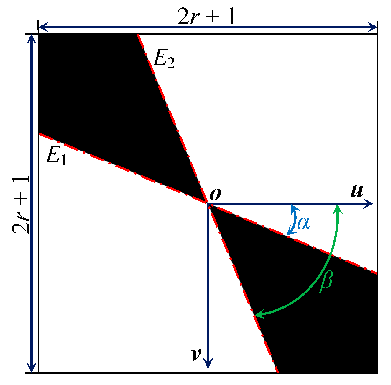
3.1. Ideally Continuous Corner Model
3.2. Sub-Pixel Corner Localization
3.3. Self-Checking for Perspective-n-Point
4. Evaluation
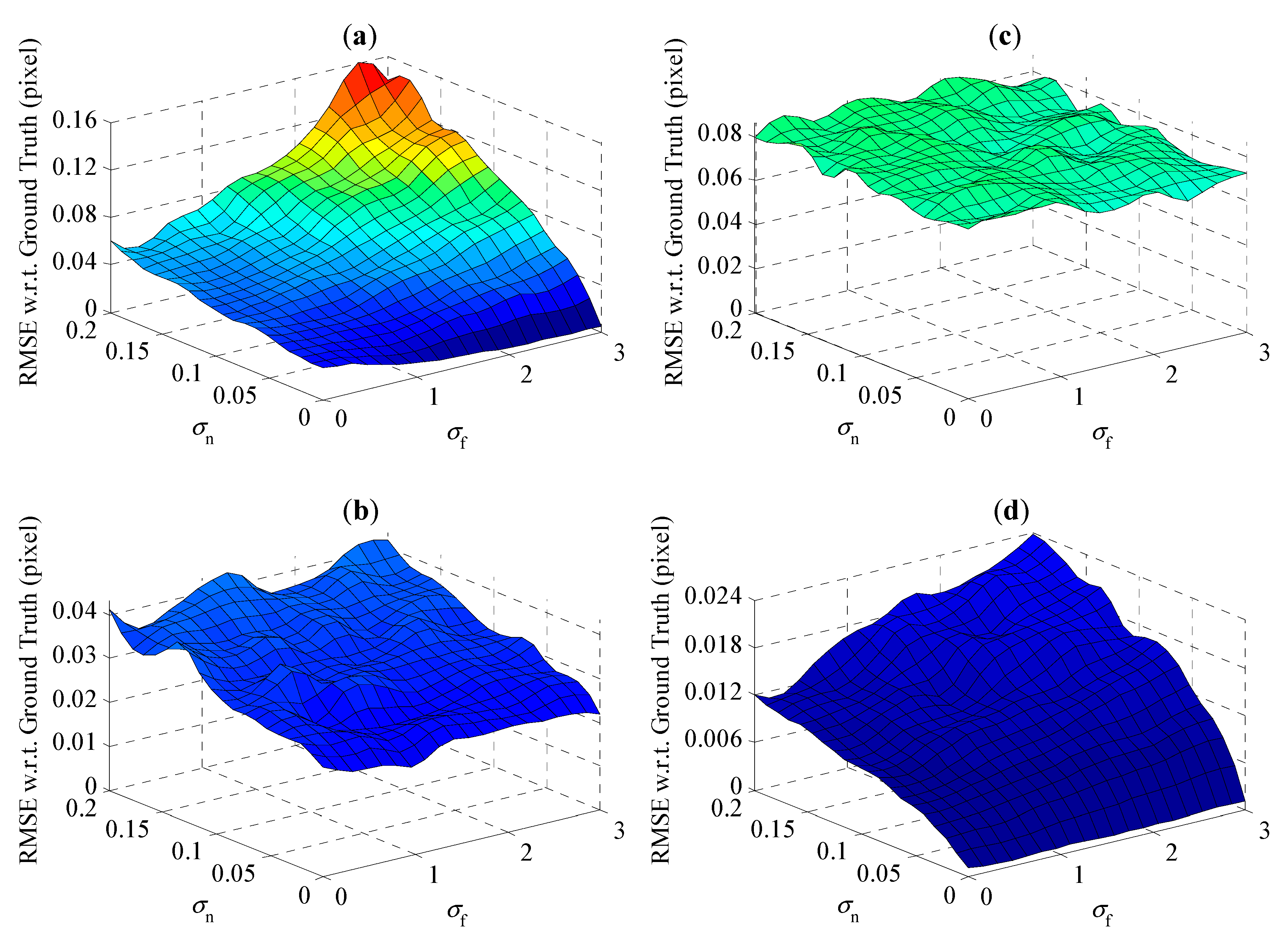
4.1. Synthetic Data
4.2. Real Data
4.3. Practical Application
4.4. Computational Efficiency Test
5. Summary
Author Contributions
Funding
Acknowledgments
Conflicts of Interest
References
- Penate-Sanchez, A.; Andrade-Cetto, J.; Moreno-Noguer, F. Exhaustive Linearization for Robust Camera Pose and Focal Length Estimation. IEEE Trans. Pattern Anal. Mach. Intell. 2013, 35, 2387–2400. [Google Scholar] [CrossRef] [PubMed]
- Zhang, Z. A flexible new technique for camera calibration. IEEE Trans. Pattern Anal. Mach. Intell. 2000, 22, 1330–1334. [Google Scholar] [CrossRef]
- Sužiedelytė-Visockienė, J. Accuracy analysis of measuring close-range image points using manual and stereo modes. Geodesy Cartogr. 2013, 39, 18–22. [Google Scholar] [CrossRef]
- Bundle Adjustment. Available online: http://en.wikipedia.org/wiki/Bundle_adjustment/ (accessed on 5 April 2018).
- Lepetit, V.; Moreno-Noguer, F.; Fua, P. EPnP: An Accurate O(n) Solution to the PnP Problem. Int. J. Comput. Vis. 2009, 81, 155–166. [Google Scholar] [CrossRef]
- Wang, Y.; Yuan, F.; Jiang, H.; Hu, Y. Novel camera calibration based on cooperative target in attitude measurement. Optik 2016, 127, 10457–10466. [Google Scholar] [CrossRef]
- Harris, C.; Stephens, M. A combined corner and edge detector. In Proceedings of the Alvey Vision Conference, Manchester, UK, 31 August–2 September 1988; pp. 147–151. [Google Scholar]
- KLT: An Implementation of the Kanade-Lucas-Tomasi Feature Tracker. Available online: http://cecas.clemson.edu/~stb/klt/ (accessed on 26 October 2018).
- Escalera, A.D.; Armingo, J.M. Automatic chessboard detection for intrinsic and extrinsic camera parameter calibration. Sensors 2010, 10, 2027–2044. [Google Scholar] [CrossRef] [PubMed]
- Tu, D.; Zhang, Y. Auto-detection of chessboard corners based on grey-level difference. Opt. Precis. Eng. 2011, 19, 1360–1365. [Google Scholar]
- Liu, Y.; Liu, S.; Cao, Y.; Wang, Z. Automatic chessboard corner detection method. IET Image Process 2016, 10, 16–23. [Google Scholar] [CrossRef]
- Yang, S.; Scherer, S.A.; Yi, X.; Zell, A. Multi-camera visual SLAM for autonomous navigation of micro aerial vehicles. Robot. Auton. Syst. 2017, 93, 116–134. [Google Scholar] [CrossRef]
- Song, L.; Wang, M.; Lu, L.; Huan, H. High precision camera calibration in vision measurement. Opt. Laser Technol. 2007, 39, 143–1420. [Google Scholar] [CrossRef]
- Zhang, T.; Liu, J.; Liu, S.; Tang, C.; Jin, P. A 3D reconstruction method for pipeline inspection based on multi-vision. Measurement 2017, 98, 35–48. [Google Scholar] [CrossRef]
- Sroba, L.; Ravas, R.; Grman, J. The Influence of Sub-pixel Corner Detection to Determine the Camera Displacement. Procedia Eng. 2015, 100, 834–840. [Google Scholar] [CrossRef]
- Bok, Y.; Ha, H.; Kweon, I.S. Automated checkerboard detection and indexing using circular boundaries. Pattern Recognit. Lett. 2016, 71, 66–72. [Google Scholar] [CrossRef]
- Camera Calibration Toolbox for Matlab. Available online: http://www.vision.caltech.edu/bouguetj/calib_doc/ (accessed on 1 September 2018).
- Camera Calibration and 3D Reconstruction. Available online: http://docs.opencv.org/2.4/modules/imgproc/doc/ (accessed on 5 September 2018).
- Chu, J.; Lu, A.G.; Wang, L. Chessboard corner detection under image physical coordinates. Opt. Laser Technol. 2013, 48, 599–605. [Google Scholar] [CrossRef]
- Zhao, Q.; Chen, Z.; Yang, T.; Zhao, Y. Detection of sub-pixel chessboard corners based on gray symmetry factor. In Proceedings of the SPIE Ninth International Symposium on Precision Engineering Measurement and Instrumentation, Changsha, China, 8–11 August 2014; Volume 9446, p. 94464S. [Google Scholar]
- Lucchese, L.; Mitra, S.K. Using saddle points for sub-pixel feature detection in camera calibration targets. In Proceedings of the Asia-Pacific Conference on Circuits and Systems, Denpasar, Indonesia, 28–31 October 2002; Volume 2, pp. 191–195. [Google Scholar]
- Chen, D.; Zhang, G. A New Sub-Pixel Detector for X-Corners in Camera Calibration Targets. In Proceedings of the 13th International Conference in Central Europe on Computer Graphics, Visualization and Computer Vision, Plzen, Czech Republic, 31 January–4 February 2005. [Google Scholar]
- Mallon, J.; Whelan, P.F. Which pattern? biasing aspects of planar calibration patterns and detection methods. Pattern Recognit. Lett. 2007, 28, 921–930. [Google Scholar] [CrossRef]
- Placht, S.; Fürsattel, P.; Mengue, E.A.; Hofmann, H.; Schaller, C.; Balda, M.; Angelopoulou, E. ROCHADE: Robust Checkerboard Advanced Detection for Camera Calibration. In Proceedings of the European Conference on Computer Vision, Zurich, Switzerland, 6–12 September 2014; Fleet, D., Pajdla, T., Schiele, B., Tuytelaars, T., Eds.; Springer: Cham, Switzerland, 2014. [Google Scholar]
- Alturki, A.S.; Loomis, J.S. X-Corner Detection for Camera Calibration Using Saddle Points. In Proceedings of the International Conference on Image Analysis and Processing, Boston, MA, USA, 25–26 April 2016. [Google Scholar]
- Wang, C.; Sun, T.; Wang, T.; Miao, X.; Wang, R. Multi-PSF fusion in image restoration of range-gated systems. Opt. Laser Technol. 2018, 103, 219–225. [Google Scholar] [CrossRef]
- Chang, S.H.; Cosman, P.C.; Milstein, L.B. Chernoff-Type Bounds for the Gaussian Error Function. IEEE Trans. Commun. 2011, 59, 2939–2944. [Google Scholar] [CrossRef]
- Wang, Z.; Wu, W. Recognition and location of the internal corners of planar checkerboard calibration pattern image. Appl. Math. Comput. 2007, 185, 894–906. [Google Scholar] [CrossRef]
- Hubert, M.; Vandervieren, E. An adjusted boxplot for skewed distribution. Comput. Stat. Data Anal. 2008, 52, 5186–5201. [Google Scholar] [CrossRef]
- Yang, T.; Zhao, Q.; Wang, X.; Huang, D. Accurate calibration approach for non-overlapping multi-camera system. Opt. Laser Technol. 2018. [Google Scholar] [CrossRef]


| gmax | gmin | yaw, pitch, roll | tx (mm) | ty (mm) | tz (mm) |
|---|---|---|---|---|---|
| [191, 255] | [0, 63] | [−π/4, π/4] | [−40, 40] | [−30, 30] | [950, 1050] |
| [u0, v0] | [fx, fy] | [k1, k2] | |
|---|---|---|---|
| [16] | [1344.42, 937.37] | [7296.06, 7298.85] | [0.2332083, 0.4313581] |
| [20] | [1342.78, 936.71] | [7298.67, 7302.12] | [0.2237942, 1.2905459] |
| [24] | [1340.02, 937.04] | [7297.59, 7300.76] | [0.2118124, 2.2750773] |
| Proposed | [1343.70, 936.62] | [7299.13, 7302.50] | [0.2253345, 0.9926340] |
| [16] | [20] | [24] | Proposed | |
|---|---|---|---|---|
| RMSD (pixel) | 0.419 | 0.287 | 0.396 | 0.241 |
| findChessboardcorners | cornerSubPix | Proposed | |
|---|---|---|---|
| Time (ms) | 41,715 | 1296 | 3051 |
© 2018 by the authors. Licensee MDPI, Basel, Switzerland. This article is an open access article distributed under the terms and conditions of the Creative Commons Attribution (CC BY) license (http://creativecommons.org/licenses/by/4.0/).
Share and Cite
Yang, T.; Zhao, Q.; Wang, X.; Zhou, Q. Sub-Pixel Chessboard Corner Localization for Camera Calibration and Pose Estimation. Appl. Sci. 2018, 8, 2118. https://doi.org/10.3390/app8112118
Yang T, Zhao Q, Wang X, Zhou Q. Sub-Pixel Chessboard Corner Localization for Camera Calibration and Pose Estimation. Applied Sciences. 2018; 8(11):2118. https://doi.org/10.3390/app8112118
Chicago/Turabian StyleYang, Tianlong, Qiancheng Zhao, Xian Wang, and Quan Zhou. 2018. "Sub-Pixel Chessboard Corner Localization for Camera Calibration and Pose Estimation" Applied Sciences 8, no. 11: 2118. https://doi.org/10.3390/app8112118
APA StyleYang, T., Zhao, Q., Wang, X., & Zhou, Q. (2018). Sub-Pixel Chessboard Corner Localization for Camera Calibration and Pose Estimation. Applied Sciences, 8(11), 2118. https://doi.org/10.3390/app8112118