An Improved Model-Based Self-Adaptive Filter for Online State-of-Charge Estimation of Li-Ion Batteries


Abstract
:1. Introduction
2. Battery Modeling
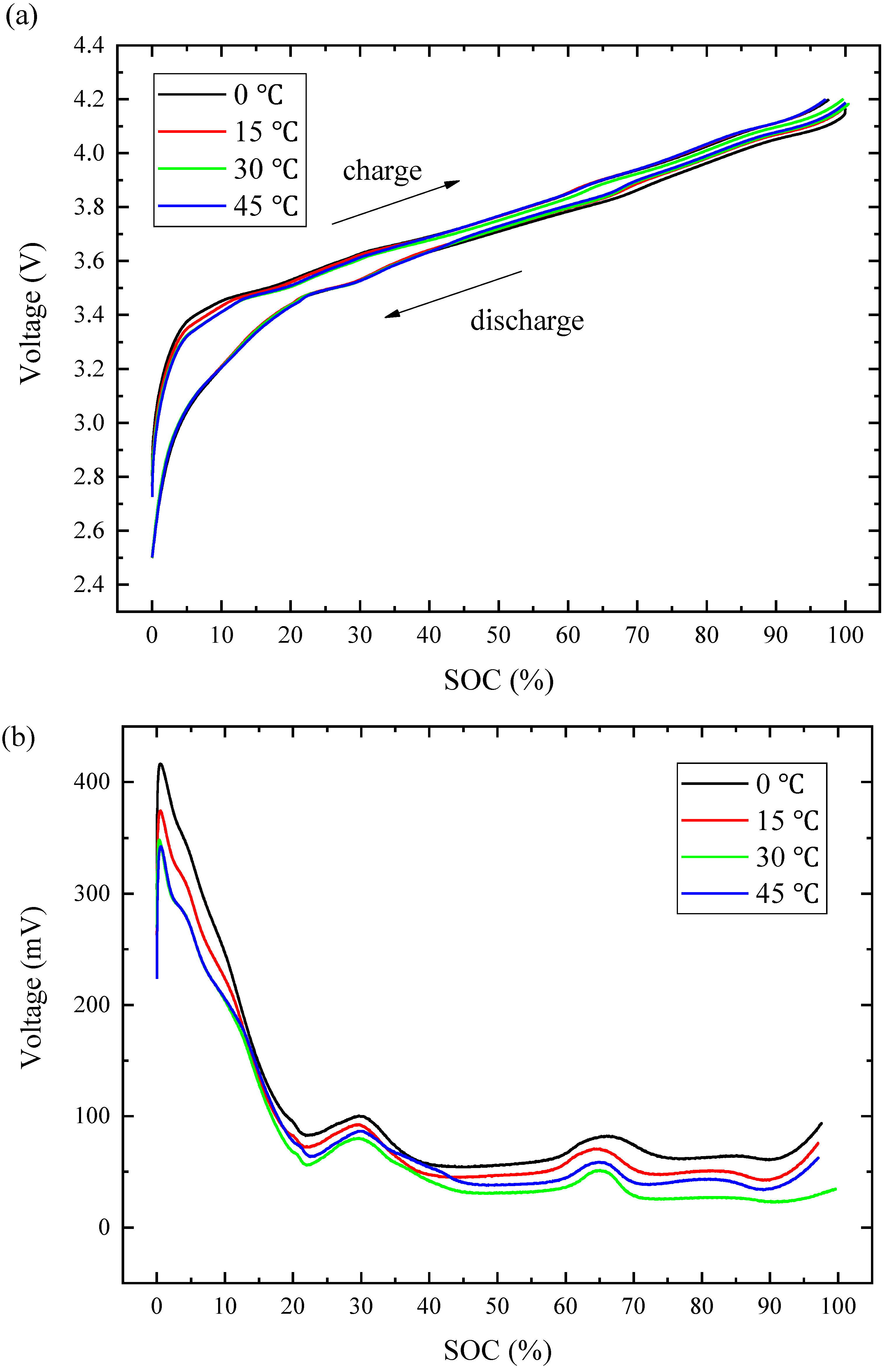
3. Battery Experiments
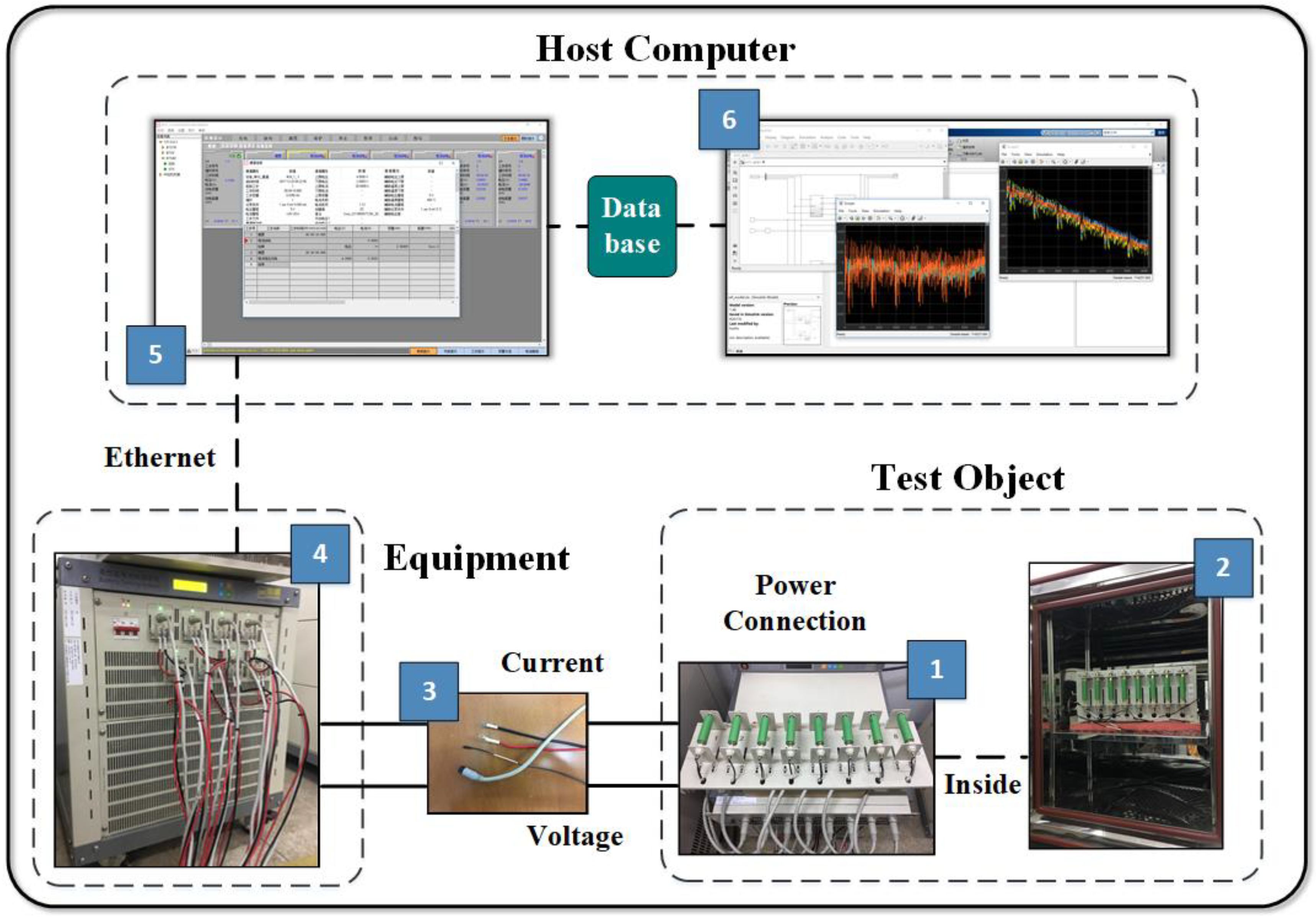
3.1. Test Bench
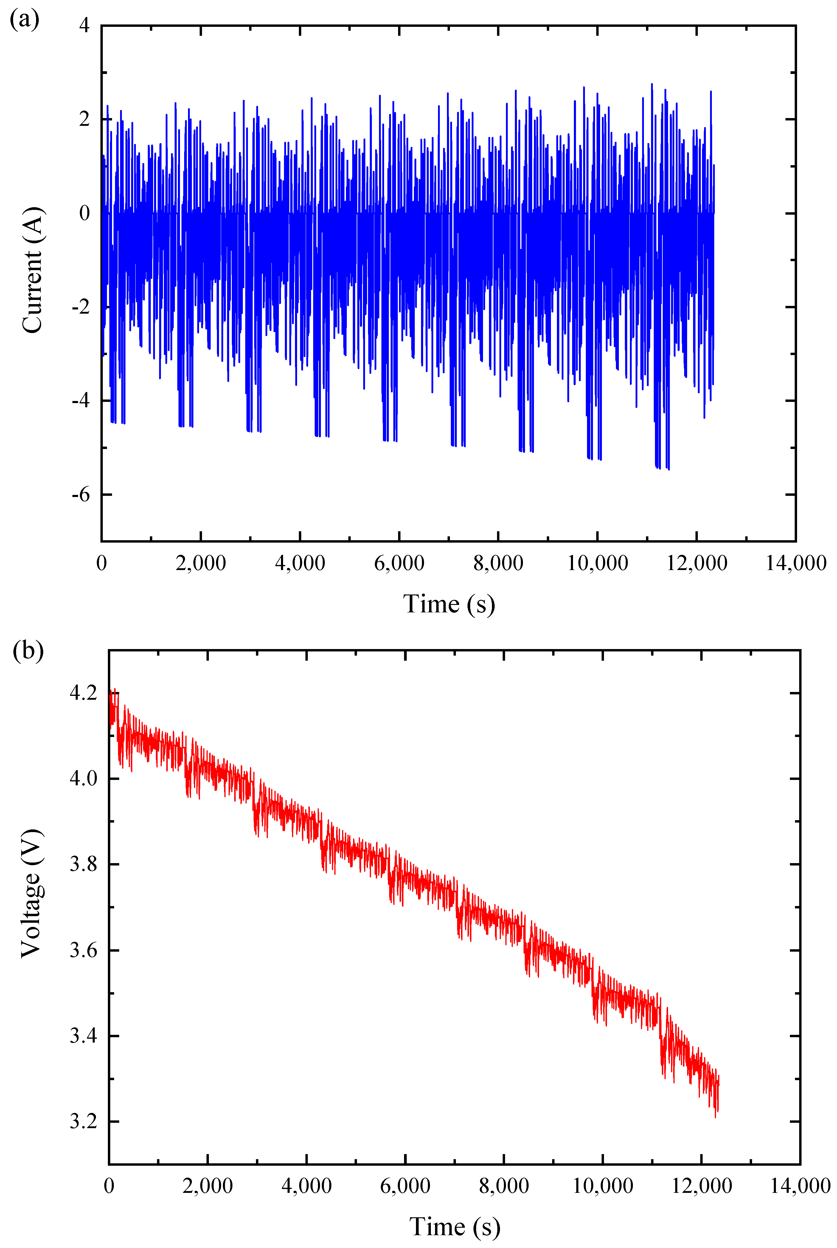
3.2. Test Schedule
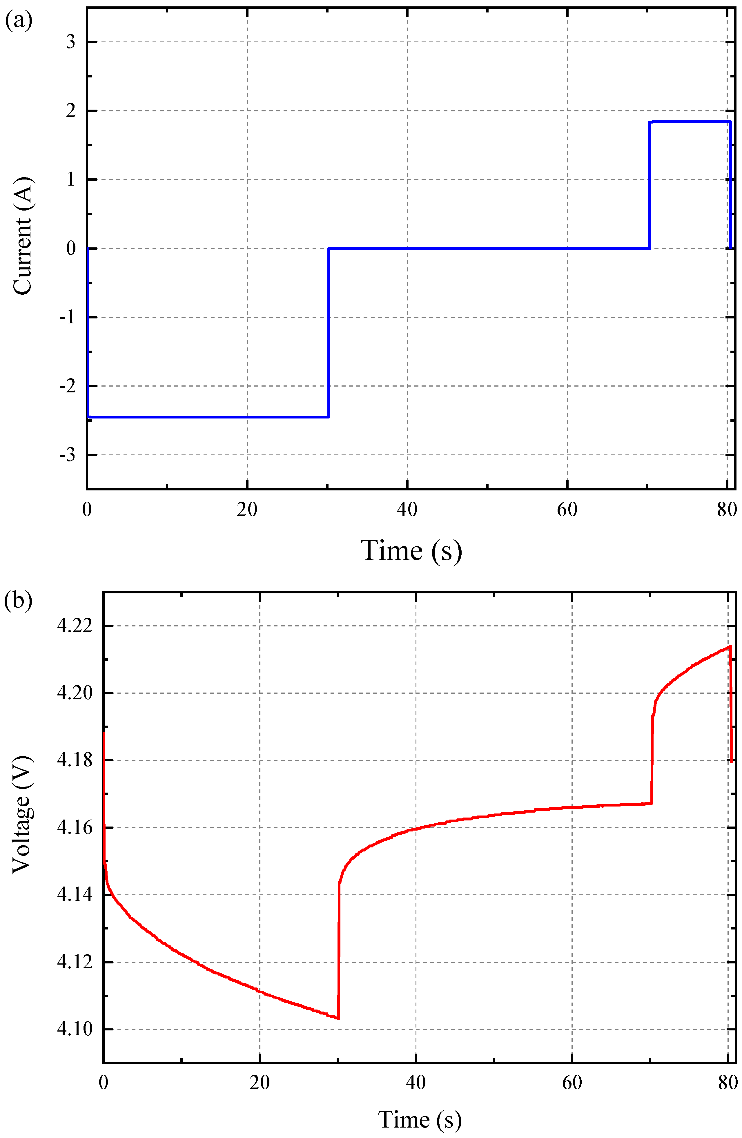
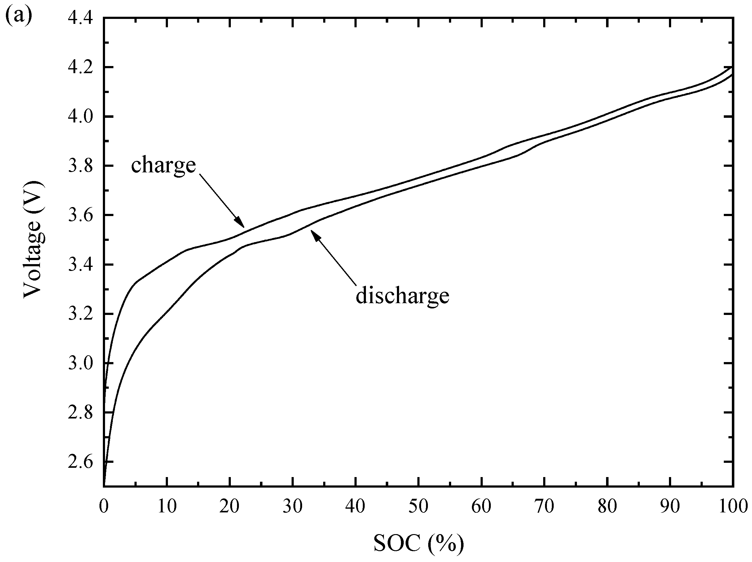
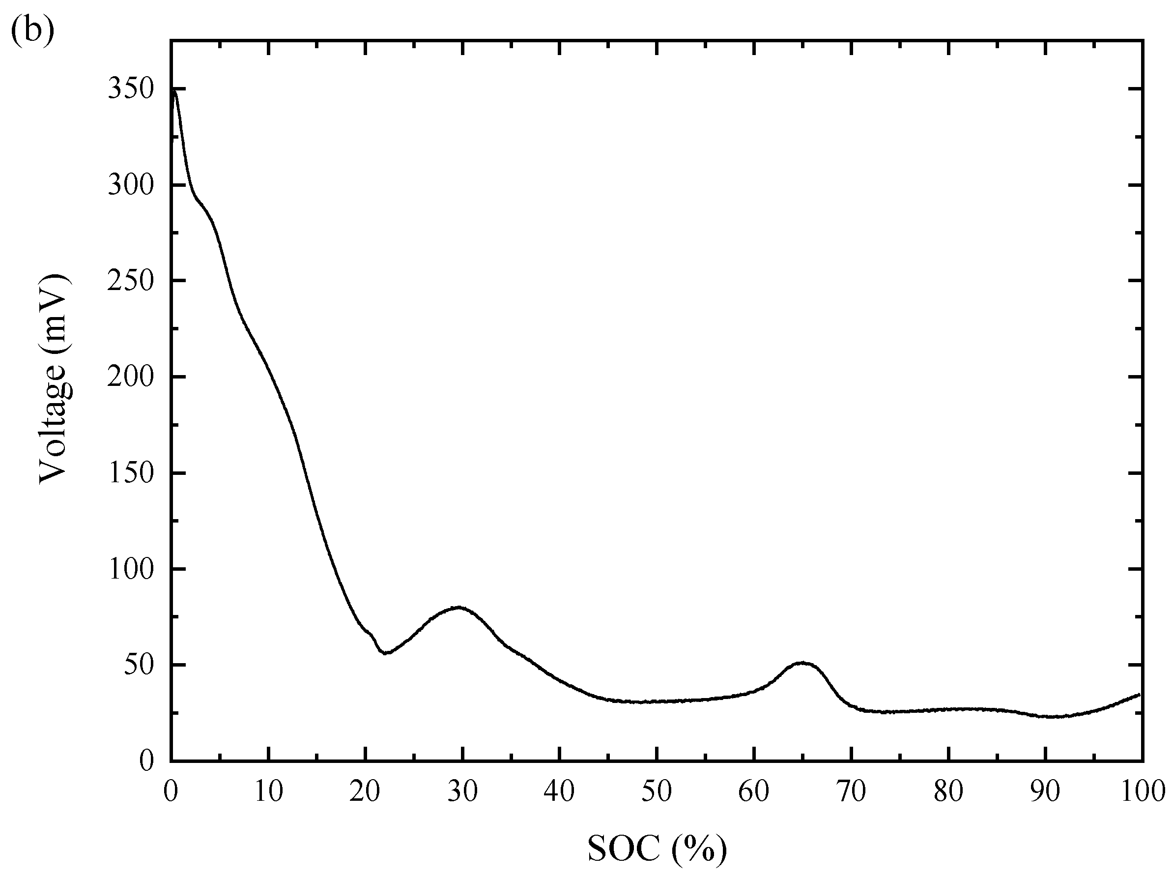
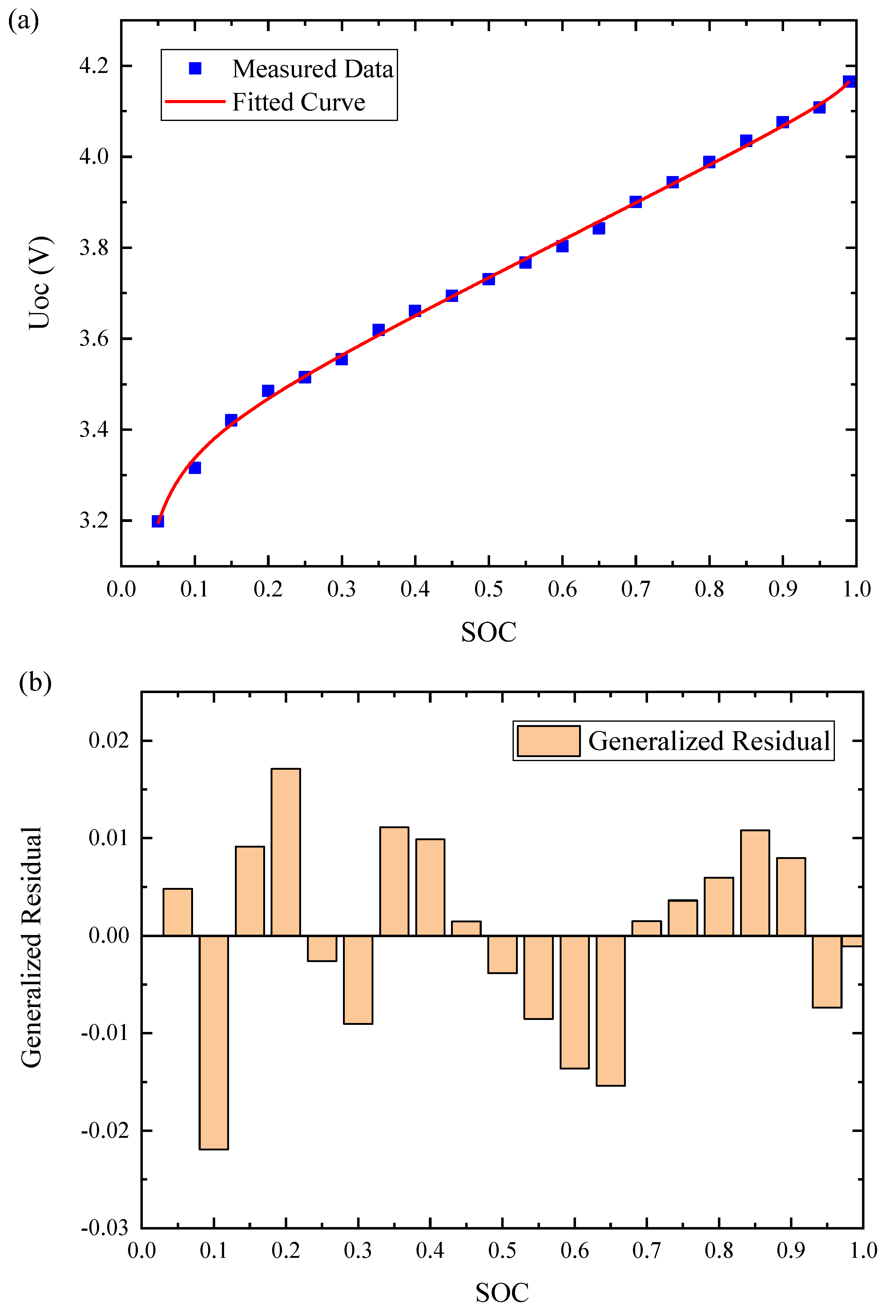
3.3. Parameters Identification
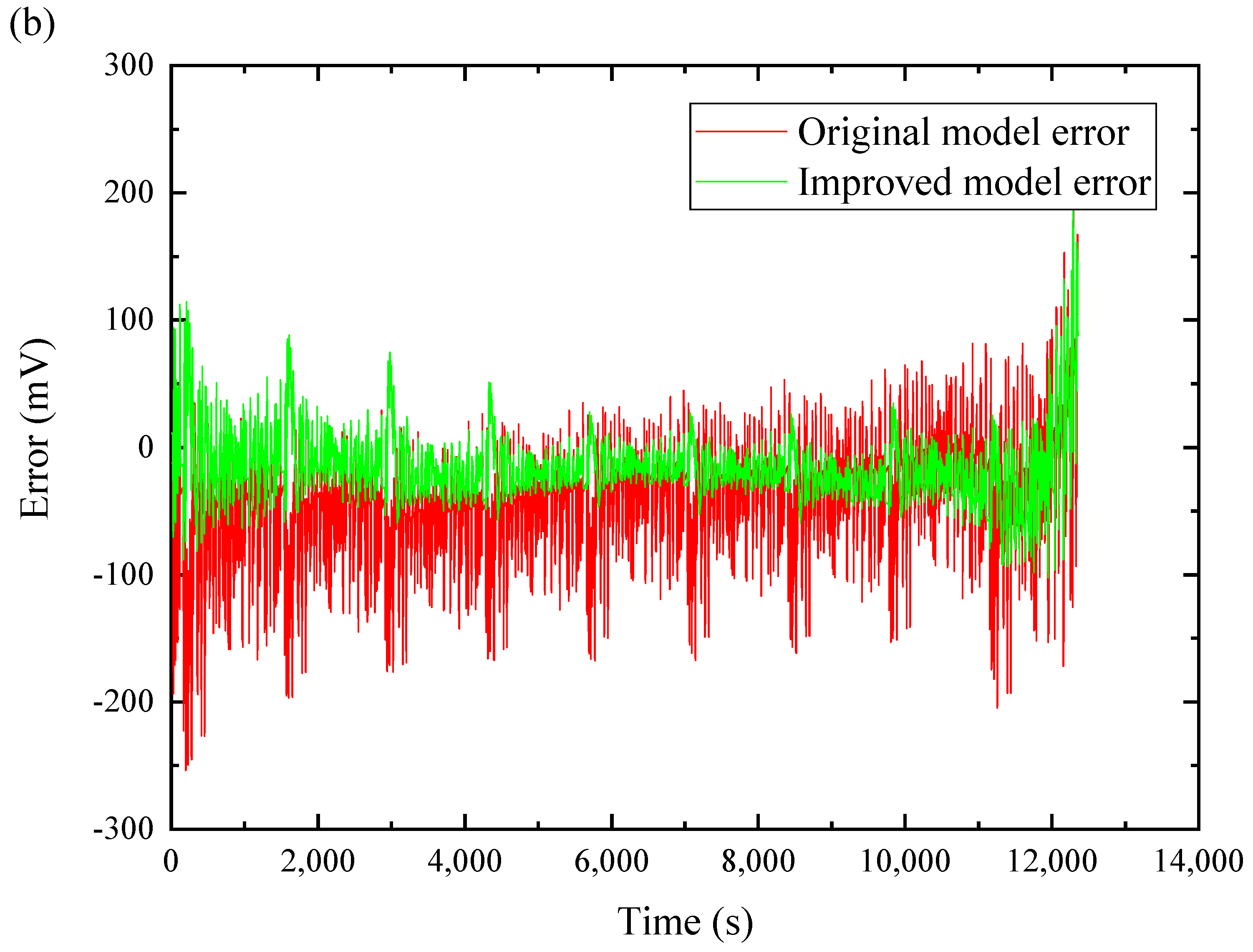
3.4. Identification Results
4. SOC Estimation Based on EKF and UKF
4.1. Extended Kalman Filtering
4.2. Unscented Kalman Filtering
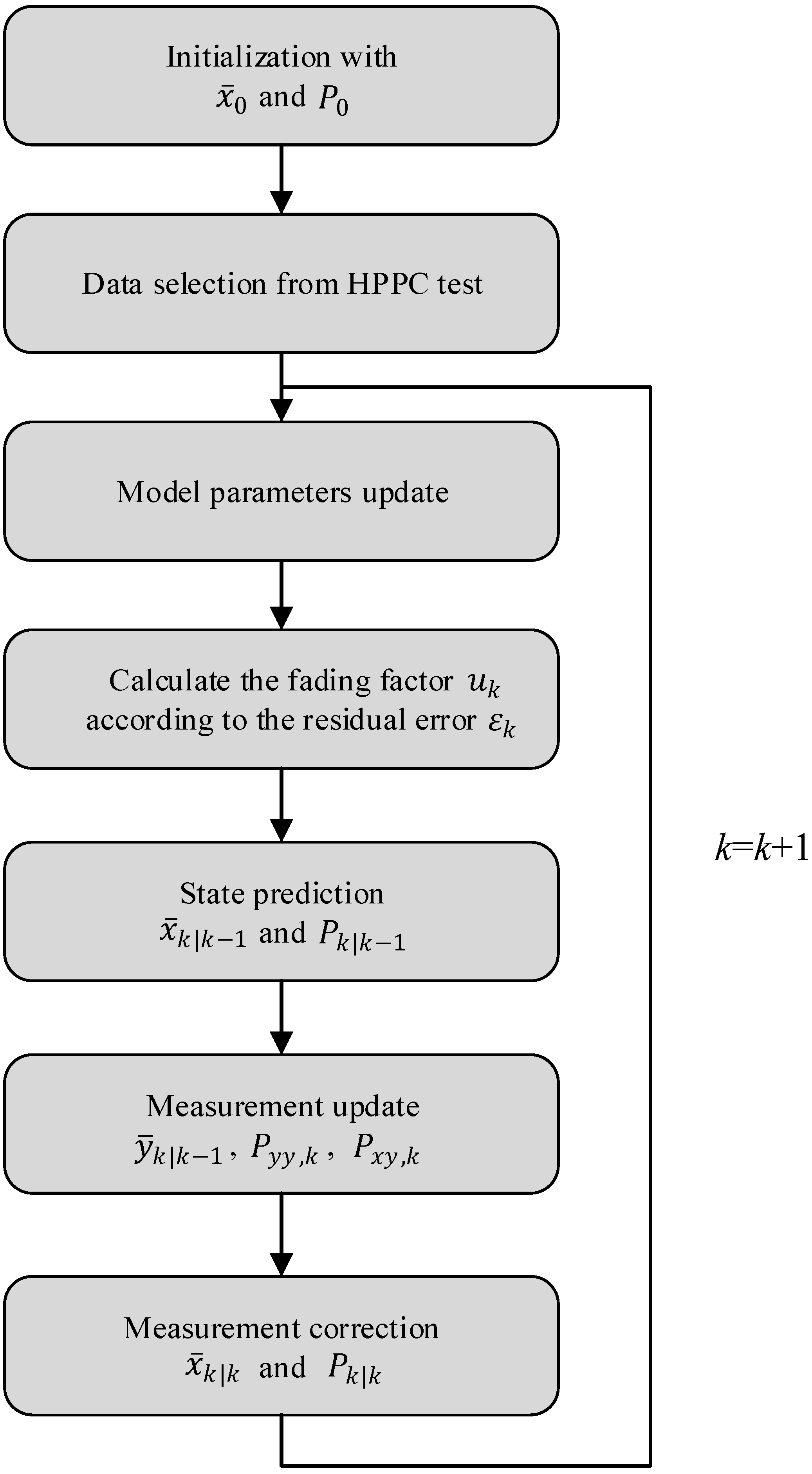
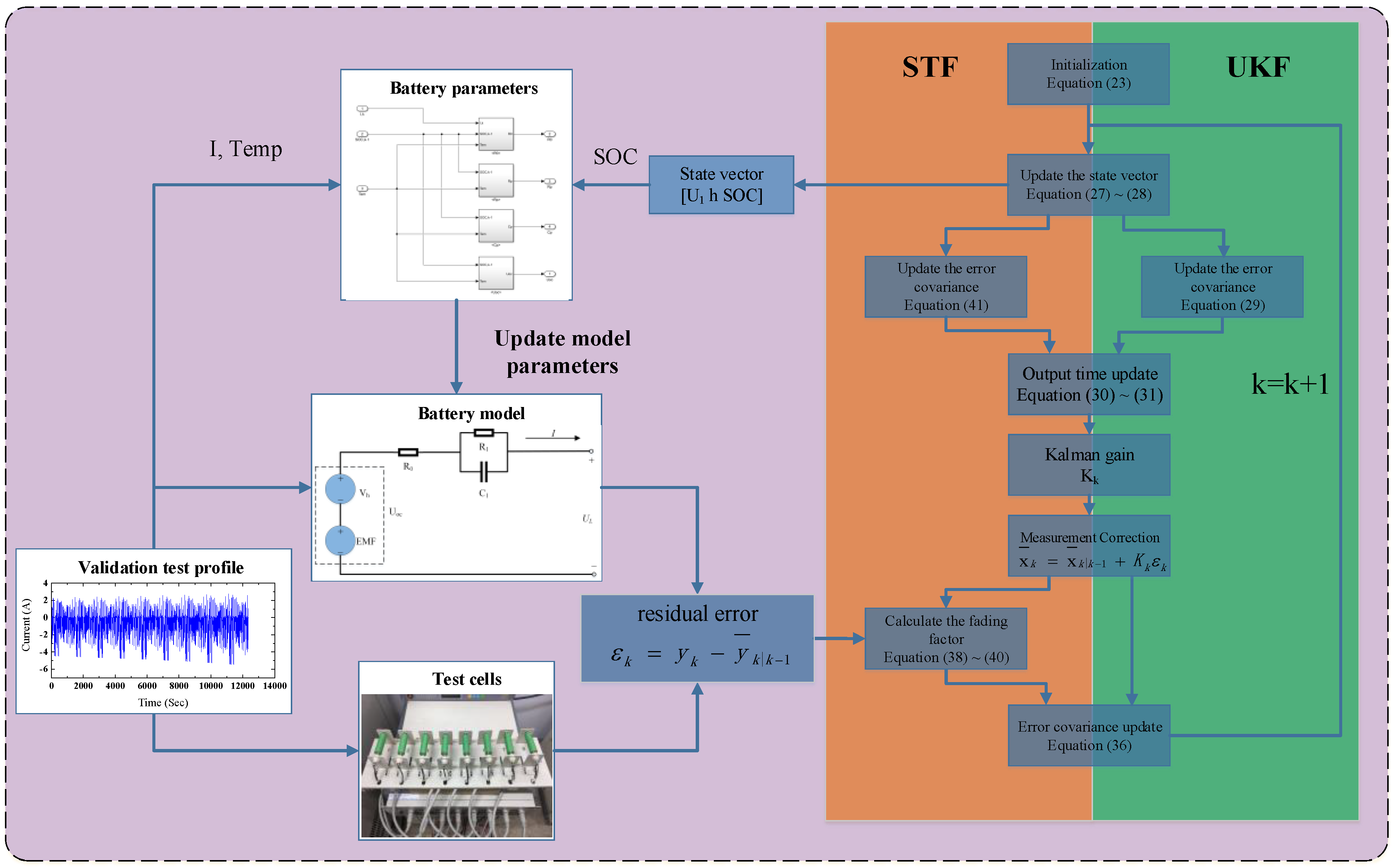
4.3. Strong Tracking Unscented Kalman Filtering
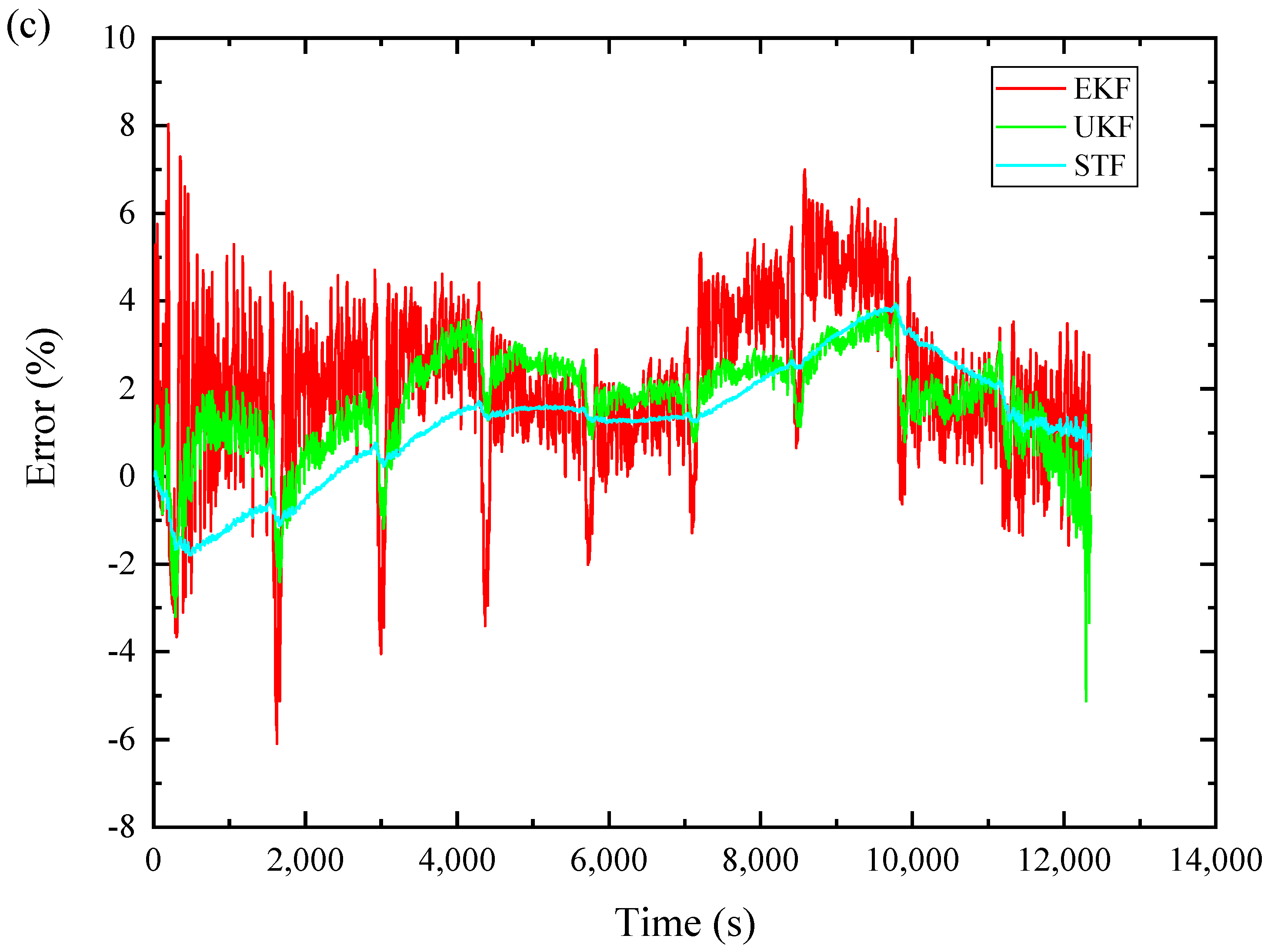
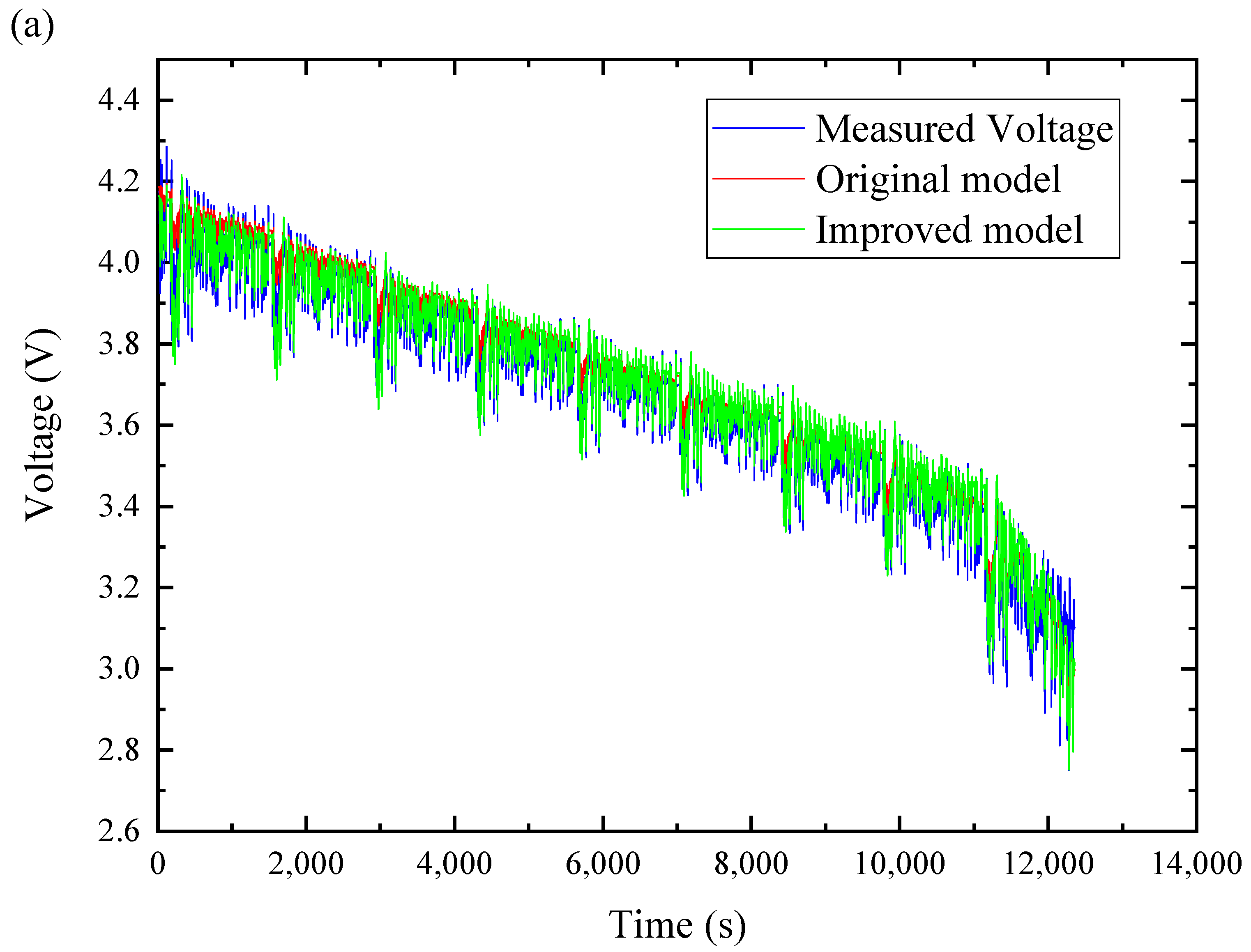
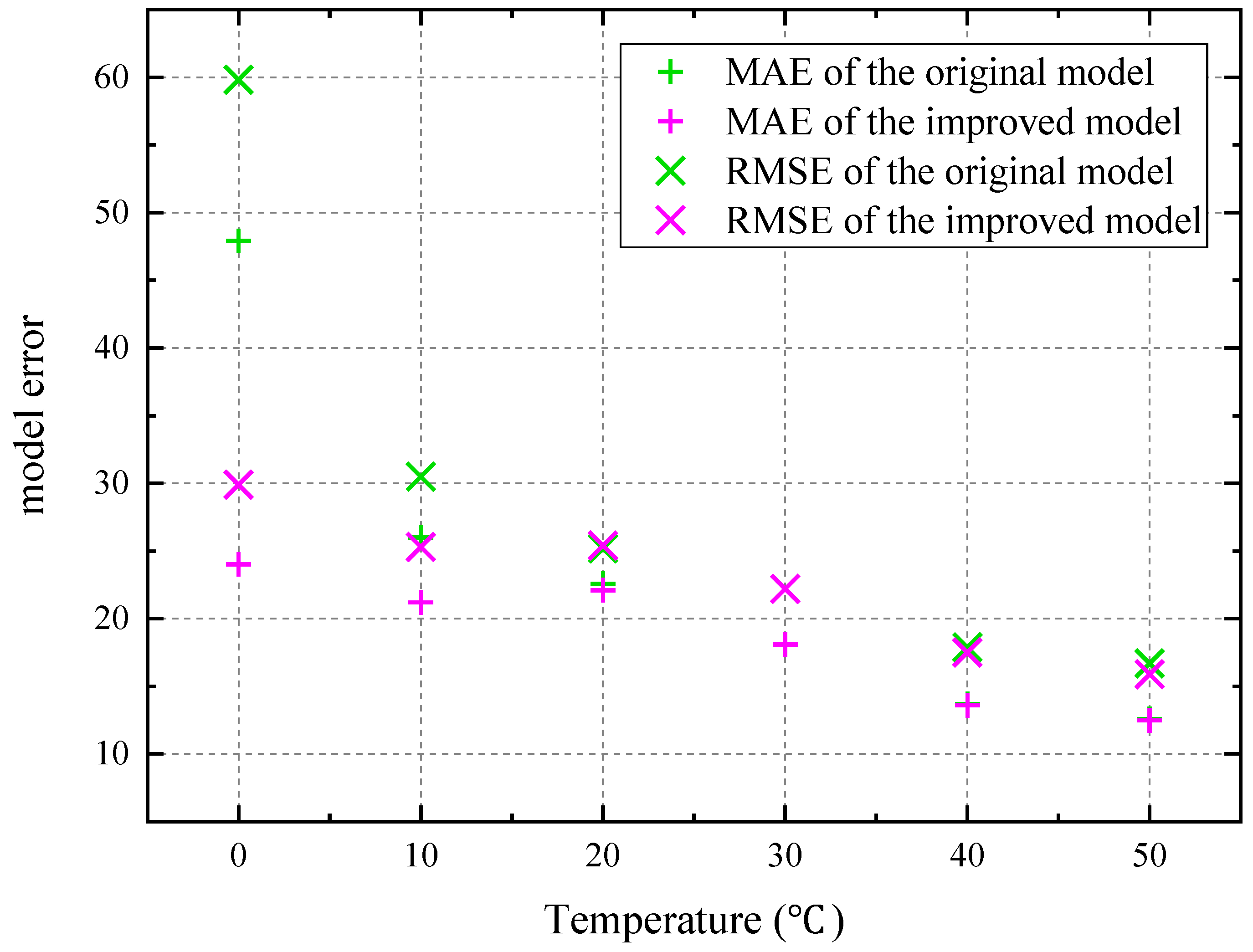
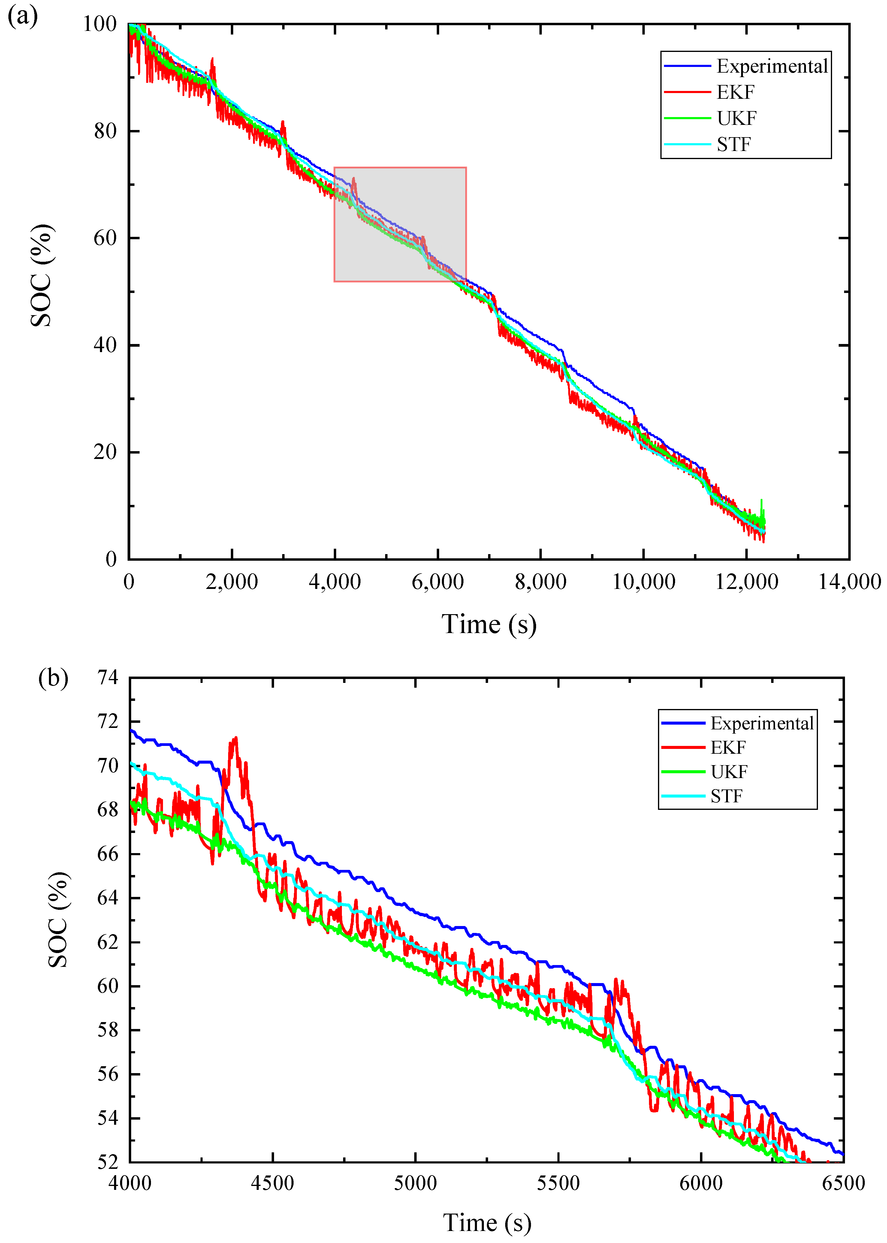
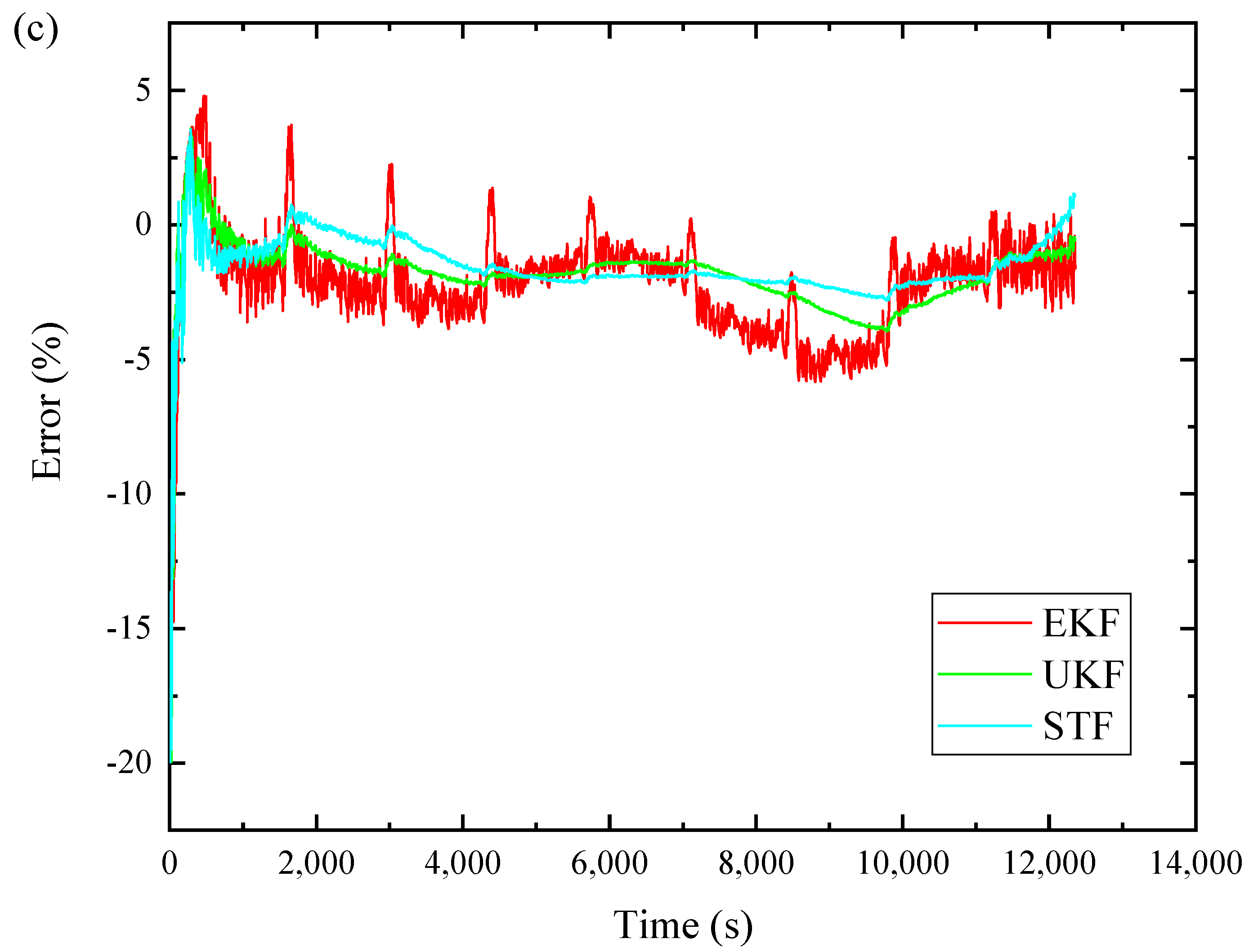
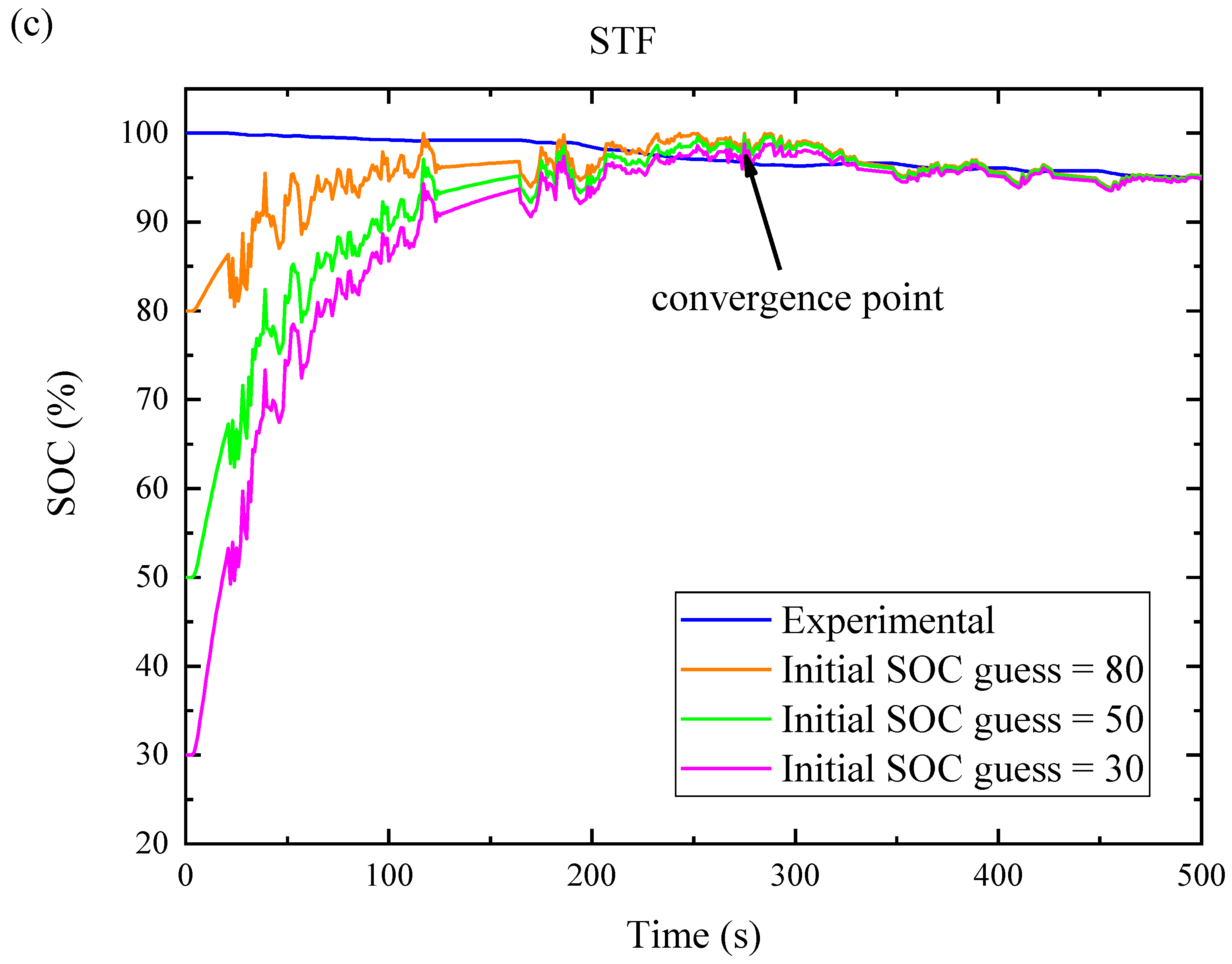
5. Results and Discussion
6. Conclusions
Author Contributions
Funding
Conflicts of Interest
Nomenclature
| CN | Battery nominal capacity |
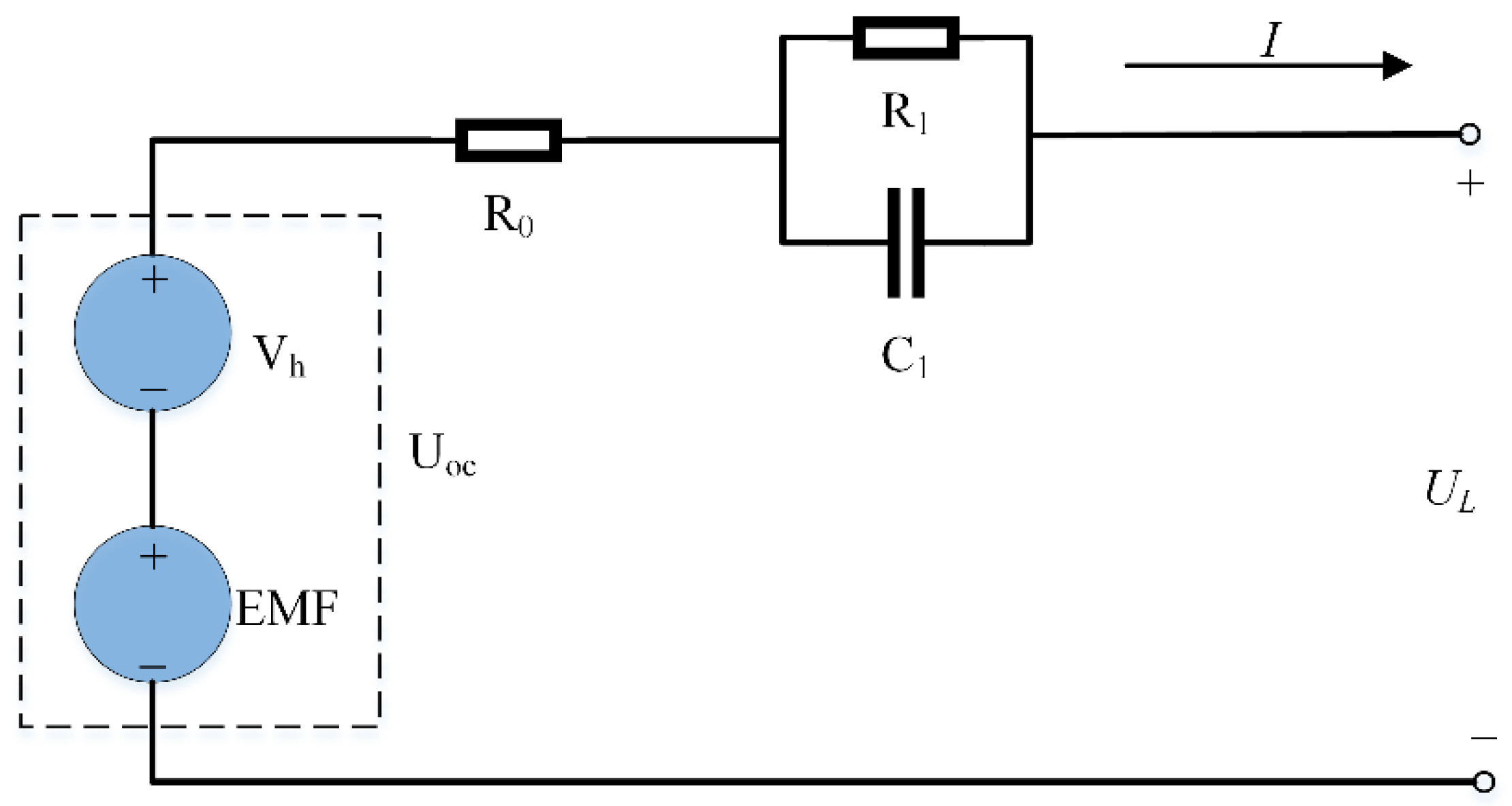
| UL | terminal voltage |
| U1 | voltage over RC network |
| Uoc | open circle voltage |
| R1 | polarization resistance |
| C1 | polarization capacitance |
| I+ | battery charge current |
| I− | battery discharge current |
| k | time step index |
| η | coulomb efficiency |
| hk | hysteresis voltage |
| γ | positive constant to tune the rate of decay |
| S(k) | experimental data (battery voltage or SOC) at step k |
| estimated value (battery voltage or SOC) at step k | |
| k|k-1 | prior estimation state |
| ωk | system process noise |
| υk | measurement noise |
| ξ | identification parameters |
| χ | a n-dimension vector for state space |
| λ | scaling parameter |
| weights of mean | |
| weights of covariance | |
| α | small positive number |
| β | state distribution parameter |
| κ | scaling factor |
| Qk | covariance matrix of the state noise |
| Rk | covariance matrix of the measurement noise |
| Kk | Kalman gain |
| εk | residual error |
| Vk | residual error sequence covariance matrix |
| μk | fading factor |
| List of abbreviations | |
| ANN | Artificial Neural Network |
| BMS | Battery Management System |
| BSF | Battery Size Factor |
| CDKF | Central-Difference Kalman filter |
| ECM | Equivalent Circuit Model |
| EKF | Extended Kalman Filter |
| EMF | Electro-Motive Force |
| EV | Electric Vehicles |
| FL | Fuzzy Logic |
| FUDS | Federal Urban Driving Schedule |
| HPPC | Hybrid Pulse Power Characterization |
| KF | Kalman filter |
| MAE | Mean Absolute Error |
| OCV | Open Circuit Voltage |
| RLS | Least Square Method |
| RMSE | Root Mean Squared Error |
| SOC | State of Charge |
| STF | Strong Tracking Filter |
| SVM | Support Vector Machine |
| UKF | Unscented Klaman Filter |
References
- Li, Z.; Huang, J.; Liaw, B.Y.; Zhang, J. On state-of-charge determination for lithium-ion batteries. J. Power Sources 2017, 348, 281–301. [Google Scholar] [CrossRef]
- Waag, W.; Fleischer, C.; Sauer, D.U. Critical review of the methods for monitoring of lithium-ion batteries in electric and hybrid vehicles. J. Power Sources 2014, 258, 321–339. [Google Scholar] [CrossRef]
- Ismail, M.M.; Hassan, M.A.M. The state of charge estimation for rechargeable batteries based on artificial neural network techniques. In Proceedings of the IEEE Control Decision and Information Technologies (CoDIT), Hammamet, Tunisia, 6–8 May 2013; pp. 733–739. [Google Scholar]
- Ismail, M.; Dlyma, R.; Elrakaybi, A. Battery state of charge estimation using an Artificial Neural Network. In Proceedings of the 2017 IEEE Transportation Electrification Conference and Expo (ITEC), Chicago, IL, USA, 22–24 June 2017. [Google Scholar]
- Burgos, C.; Sáez, D.; Orchard, M.E.; Cárdenas, R. Fuzzy modelling for the state-of-charge estimation of lead-acid batteries. J. Power Sources 2015, 274, 355–366. [Google Scholar] [CrossRef]
- Jiani, D.; Zhitao, L.; Youyi, W. A fuzzy logic-based model for Li-ion battery with SOC and temperature effect. In Proceedings of the 11th IEEE Control & Automation (ICCA), Taichung, Taiwan, 18–20 June 2014; pp. 1333–1338. [Google Scholar]
- Álvarez Antón, J.C.; García Nieto, P.J.; de Cos Juez, F.J.; Sánchez Lasheras, F.; González Vega, M.; Roqueñí Gutiérrez, M.N. Battery state-of-charge estimator using the SVM technique. Appl. Math. Modell. 2013, 37, 6244–6253. [Google Scholar] [CrossRef]
- Hansen, T.; Wang, C.-J. Support vector based battery state of charge estimator. J. Power Sources 2005, 141, 351–358. [Google Scholar] [CrossRef]
- Sheng, H.; Xiao, J. Electric vehicle state of charge estimation: Nonlinear correlation and fuzzy support vector machine. J. Power Sources 2015, 281, 131–137. [Google Scholar] [CrossRef]
- Surendar, V.; Mohankumar, V.; Anand, S.; Prasanna, V.D. Estimation of State of Charge of a Lead Acid Battery Using Support Vector Regression. Procedia Technol. 2015, 21, 264–270. [Google Scholar] [CrossRef]
- Alvarez Anton, J.C.; Garcia Nieto, P.J.; Blanco Viejo, C.; Vilan Vilan, J.A. Support Vector Machines Used to Estimate the Battery State of Charge. IEEE Trans. Power Electron. 2013, 28, 5919–5926. [Google Scholar] [CrossRef]
- Campestrini, C.; Horsche, M.F.; Zilberman, I.; Heil, T.; Zimmermann, T.; Jossen, A. Validation and benchmark methods for battery management system functionalities: State of charge estimation algorithms. J. Energy Storage 2016, 7, 38–51. [Google Scholar] [CrossRef]
- Plett, G.L. Extended Kalman filtering for battery management systems of LiPB-based HEV battery packs Part 1. Background. J. Power Sources 2004, 134, 252–261. [Google Scholar] [CrossRef]
- Plett, G.L. Extended Kalman filtering for battery management systems of LiPB-based HEV battery packs Part 2. Modeling and identification. J. Power Sources 2004, 134, 262–276. [Google Scholar] [CrossRef]
- Plett, G.L. Extended Kalman filtering for battery management systems of LiPB-based HEV battery packs Part 3. State and parameter estimation. J. Power Sources 2004, 134, 277–292. [Google Scholar] [CrossRef]
- Plett, G.L. High-Performance Battery-Pack Power Estimation Using a Dynamic Cell Model. IEEE Trans. Veh. Technol. 2004, 53, 1586–1593. [Google Scholar] [CrossRef] [Green Version]
- Dai, H.; Sun, Z.; Wei, X. Online SOC Estimation of High-power Lithium-ion Batteries Used on HEVs. IEEE Veh. Electron. Saf. 2006, 342–347. [Google Scholar]
- Mastali, M.; Vazquez-Arenas, J.; Fraser, R.; Fowler, M.; Afshar, S.; Stevens, M. Battery state of the charge estimation using Kalman filtering. J. Power Sources 2013, 239, 294–307. [Google Scholar] [CrossRef]
- Sepasi, S.; Ghorbani, R.; Liaw, B.Y. Improved extended Kalman filter for state of charge estimation of battery pack. J. Power Sources 2014, 255, 368–376. [Google Scholar] [CrossRef]
- Pérez, G.; Garmendia, M.; Reynaud, J.F.; Crego, J.; Viscarret, U. Enhanced closed loop State of Charge estimator for lithium-ion batteries based on Extended Kalman Filter. Appl. Energy 2015, 155, 834–845. [Google Scholar] [CrossRef]
- Pan, H.; Lü, Z.; Lin, W.; Li, J.; Chen, L. State of charge estimation of lithium-ion batteries using a grey extended Kalman filter and a novel open-circuit voltage model. Energy 2017, 138, 764–775. [Google Scholar] [CrossRef]
- Li, Z.; Zhang, P.; Wang, Z.; Song, Q.; Rong, Y. State of Charge Estimation for Li-ion Battery Based on Extended Kalman Filter. Energy Procedia 2017, 105, 3515–3520. [Google Scholar]
- Sun, F.; Hu, X.; Zou, Y.; Li, S. Adaptive unscented Kalman filtering for state of charge estimation of a lithium-ion battery for electric vehicles. Energy 2011, 36, 3531–3540. [Google Scholar] [CrossRef]
- Xiong, R.; Gong, X.; Mi, C.C.; Sun, F. A robust state-of-charge estimator for multiple types of lithium-ion batteries using adaptive extended Kalman filter. J. Power Sources 2013, 243, 805–816. [Google Scholar] [CrossRef]
- Roscher, M.A.; Sauer, D.U. Dynamic electric behavior and open-circuit-voltage modeling of LiFePO4-based lithium ion secondary batteries. J. Power Sources 2011, 196, 331–336. [Google Scholar] [CrossRef]
- García-Plaza, M.; Eloy-García Carrasco, J.; Peña-Asensio, A.; Alonso-Martínez, J.; Arnaltes Gómez, S. Hysteresis effect influence on electrochemical battery modeling. Electr. Power Syst. Res. 2017, 152, 27–35. [Google Scholar] [CrossRef]
- Dong, G.; Wei, J.; Zhang, C.; Chen, Z. Online state of charge estimation and open circuit voltage hysteresis modeling of LiFePO 4 battery using invariant imbedding method. Appl. Energy 2016, 162, 163–171. [Google Scholar] [CrossRef]
- Li, H.; Song, Y.; Lu, B.; Zhang, J. Effects of stress dependent electrochemical reaction on voltage hysteresis of lithium ion batteries. Appl. Math. Mech. 2018, 39, 1453–1464. [Google Scholar] [CrossRef]
- Christopherson, J.P. Battery Test Manual For Electric Vehicles; Idaho National Laboratory: Idaho Falls, ID, USA, 2015. [Google Scholar]
- Li, Y.; Wang, C.; Gong, J. A combination Kalman filter approach for State of Charge estimation of lithium-ion battery considering model uncertainty. Energy 2016, 109, 933–946. [Google Scholar] [CrossRef]
- Xiong, R.; Sun, F.; Gong, X.; Gao, C. A data-driven based adaptive state of charge estimator of lithium-ion polymer battery used in electric vehicles. Appl. Energy 2014, 113, 1421–1433. [Google Scholar] [CrossRef]
- Li, D.; Ouyang, J.; Li, H.; Wan, J. State of charge estimation for LiMn2O4 power battery based on strong tracking sigma point Kalman filter. J. Power Sources 2015, 279, 439–449. [Google Scholar] [CrossRef]


| Item | Rating |
|---|---|
| Capacity | 2.5 Ah |
| End of discharge voltage | 2.5 V |
| Maximum charge voltage | 4.2 V |
| Maximum discharge current rate | 12 C |
| Initialization |
| 1. Initialize with: , |
| State prediction |
| 1. Update the step state vector: |
| 2. Update the step error covariance: |
| Measurement update |
| 1. Calculate the Kalman gain: |
| 2. Update the measurement vector: |
| 3. Update the error covariance: |
| Initialization |
| 1. Initialize with: |
| State prediction |
| 1. Update the step state vector: |
| 2. Update the step error covariance: |
| Measurement update |
| 1. Output estimate time update: |
| 2. Calculate prediction covariance: 3. Calculate cross-covariance covariance: |
| Measurement correction |
| 1. Calculate the Kalman gain: 2. State estimate measurement update: 3. Error covariance measurement update: |
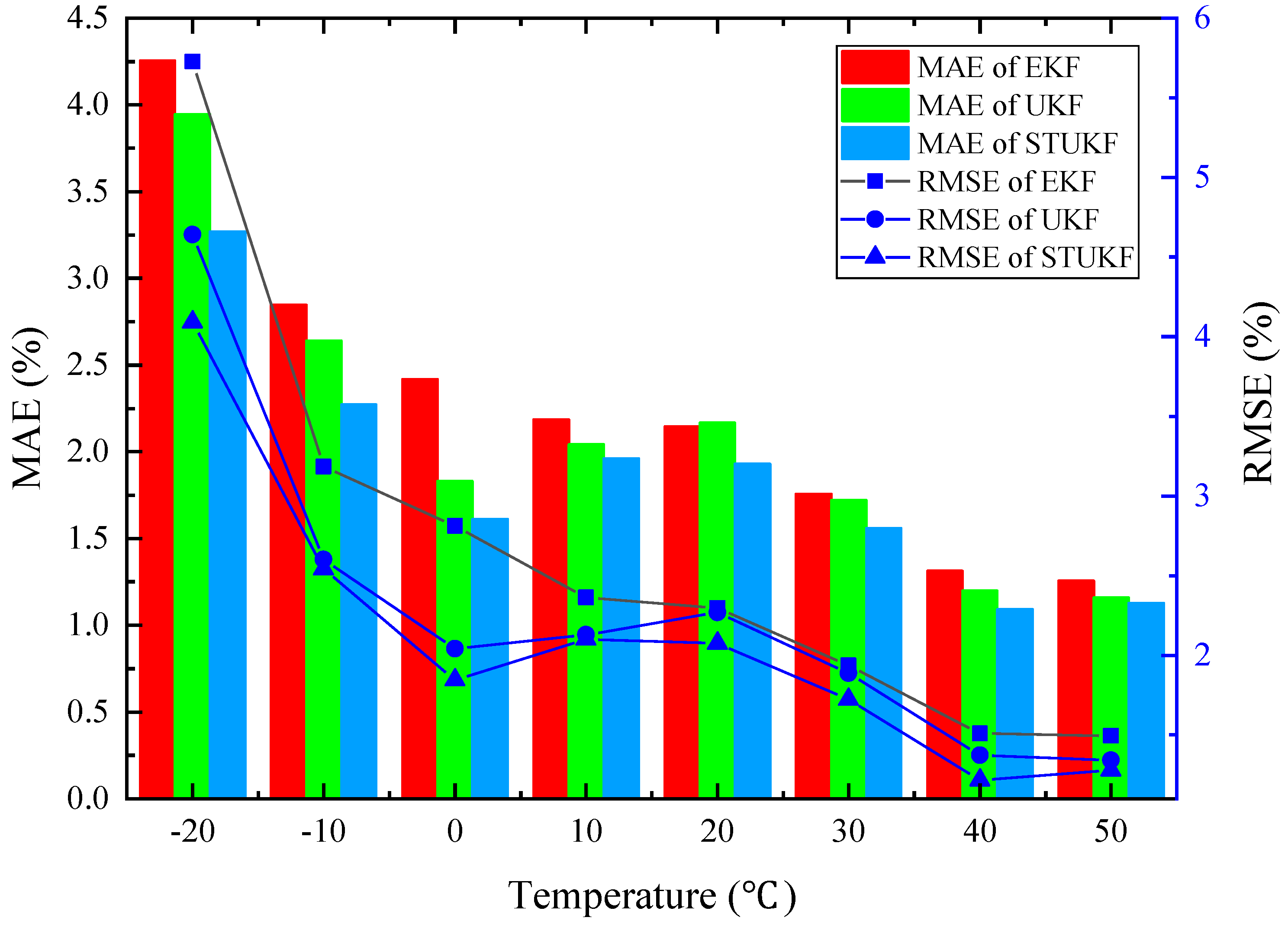
| MAE | ||||||||
| −20 °C | −10 °C | 0 °C | 10 °C | 20 °C | 30 °C | 40 °C | 50 °C | |
| EKF | 4.2556 | 2.8469 | 2.4179 | 2.1860 | 2.1458 | 1.7587 | 1.3136 | 1.2558 |
| UKF | 3.9459 | 2.6408 | 1.8307 | 2.0419 | 2.1688 | 1.7202 | 1.1985 | 1.1593 |
| STF | 3.2692 | 2.2711 | 1.6102 | 1.9618 | 1.9292 | 1.5580 | 1.0925 | 1.1274 |
| RMSE | ||||||||
| −20 °C | −10 °C | 0 °C | 10 °C | 20 °C | 30 °C | 40 °C | 50 °C | |
| EKF | 5.7263 | 3.1847 | 2.8112 | 2.3636 | 2.2978 | 1.9360 | 1.5081 | 1.4964 |
| UKF | 4.6393 | 2.6023 | 2.0419 | 2.1297 | 2.2687 | 1.8886 | 1.3736 | 1.3426 |
| STF | 4.0924 | 2.5410 | 1.8461 | 2.1017 | 2.0763 | 1.7240 | 1.2160 | 1.2795 |
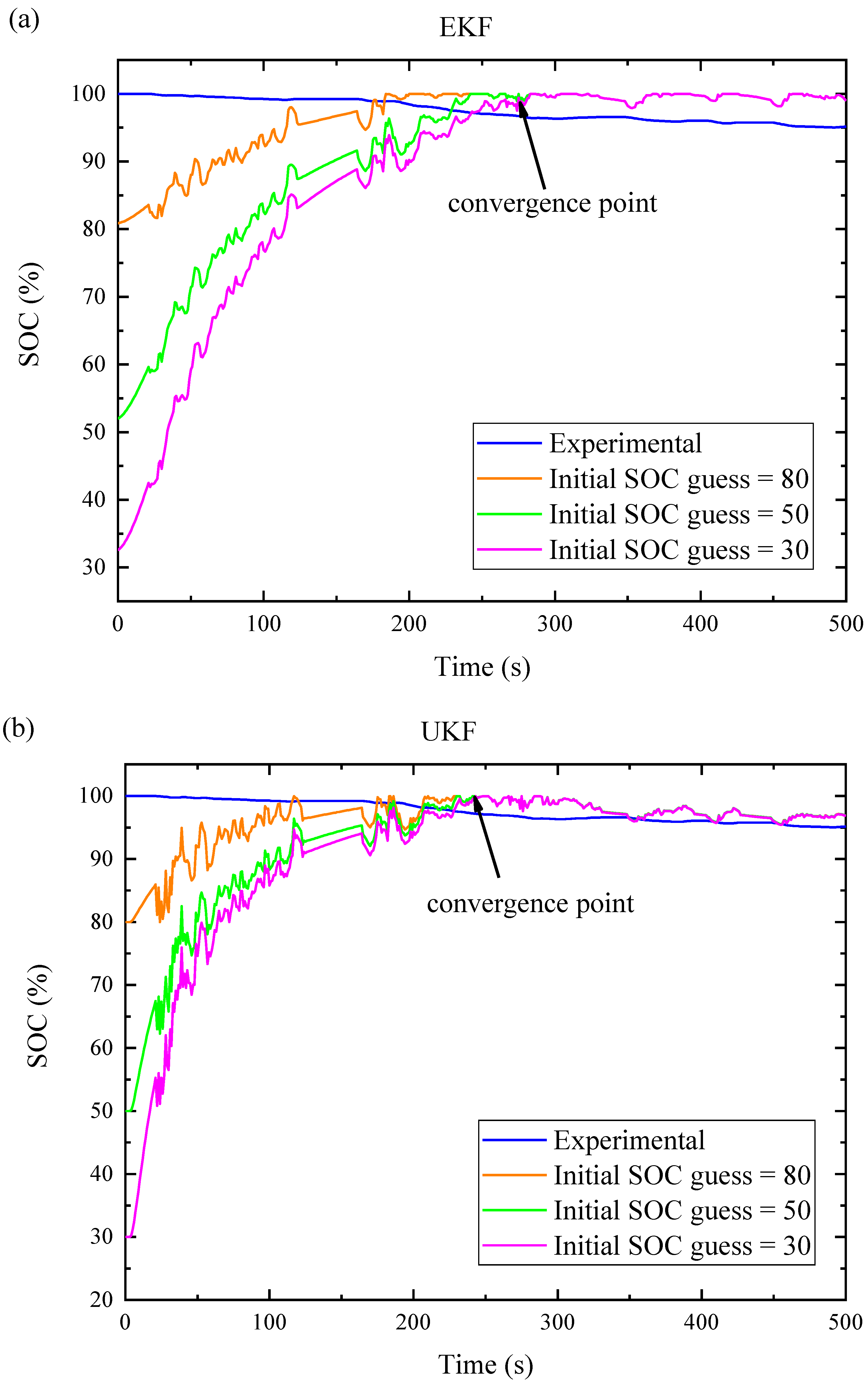
| MAE | |||
| Initial SOC Guess (%) | EKF | UKF | STF |
| 80 | 2.431 | 1.906 | 1.603 |
| 50 | 2.632 | 2.043 | 1.732 |
| 30 | 2.761 | 2.122 | 1.826 |
| RMSE | |||
| Initial SOC Guess (%) | EKF | UKF | STF |
| 80 | 2.936 | 2.260 | 1.980 |
| 50 | 4.045 | 3.173 | 2.967 |
| 30 | 5.032 | 3.884 | 3.805 |
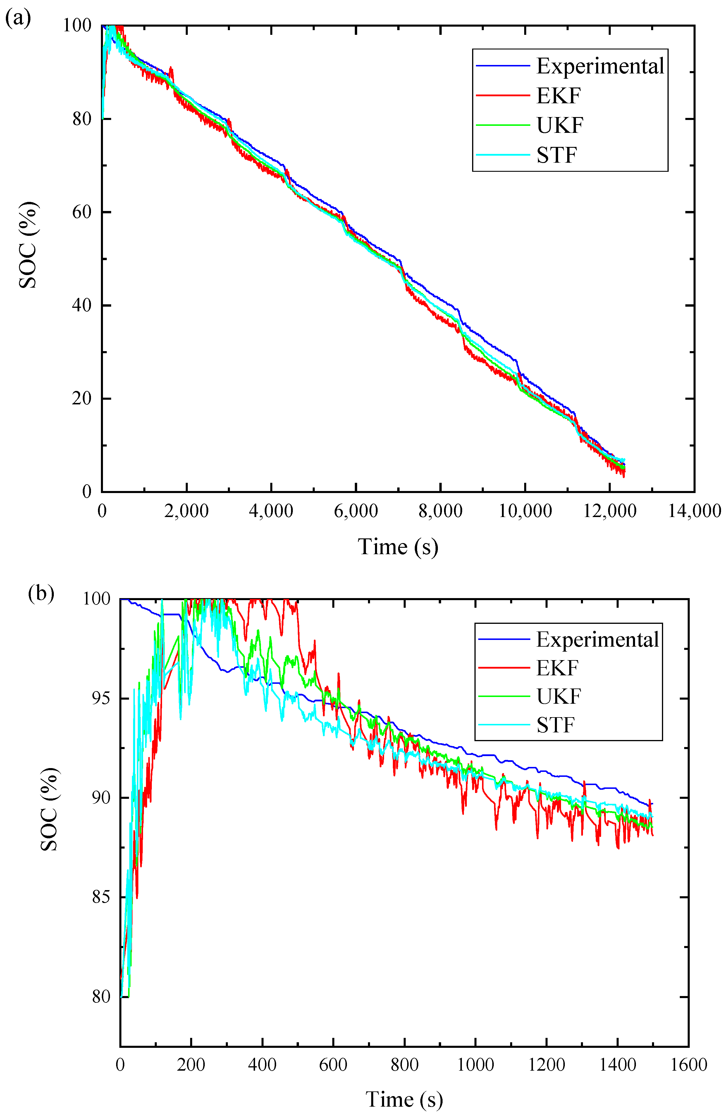
| Algorithm | MAE (%) | RMSE (%) |
|---|---|---|
| EKF | 2.262 | 2.385 |
| UKF | 2.222 | 2.305 |
| STF | 2.186 | 2.280 |
© 2018 by the authors. Licensee MDPI, Basel, Switzerland. This article is an open access article distributed under the terms and conditions of the Creative Commons Attribution (CC BY) license (http://creativecommons.org/licenses/by/4.0/).
Share and Cite
Zhang, C.; Yan, F.; Du, C.; Rizzoni, G. An Improved Model-Based Self-Adaptive Filter for Online State-of-Charge Estimation of Li-Ion Batteries. Appl. Sci. 2018, 8, 2084. https://doi.org/10.3390/app8112084
Zhang C, Yan F, Du C, Rizzoni G. An Improved Model-Based Self-Adaptive Filter for Online State-of-Charge Estimation of Li-Ion Batteries. Applied Sciences. 2018; 8(11):2084. https://doi.org/10.3390/app8112084
Chicago/Turabian StyleZhang, Chi, Fuwu Yan, Changqing Du, and Giorgio Rizzoni. 2018. "An Improved Model-Based Self-Adaptive Filter for Online State-of-Charge Estimation of Li-Ion Batteries" Applied Sciences 8, no. 11: 2084. https://doi.org/10.3390/app8112084
APA StyleZhang, C., Yan, F., Du, C., & Rizzoni, G. (2018). An Improved Model-Based Self-Adaptive Filter for Online State-of-Charge Estimation of Li-Ion Batteries. Applied Sciences, 8(11), 2084. https://doi.org/10.3390/app8112084