Featured Application
Paper compares the adaptive non-linear controller using the evolution strategies with the linear PI-controller on a non-linear robotic control plant.
Abstract
The majority of non-linear systems nowadays are controlled online using rapid PI-controllers with linear characteristics. Evolutionary algorithms are rarely used, especially for online adaptive control, due to their time complexity. This paper proposes an online adaptive controller based on a dynamic evolution strategy and attempts to overcome this performance problem. The main advantage of the evolution strategies over other gradient machine learning algorithms is that they are insensitive to becoming stuck into local optima. As a result, the proposed controller is capable of responding in real-time (sampling time between 1–5 ms) and was tested on a non-linear, single-degree-of-freedom robotic mechanism. To the extent of our knowledge, this is the first application of evolutionary algorithms in such an online control. In general, the results obtained were better than the results achieved using a traditional PI-controller.
1. Introduction
Evolutionary Algorithms (EAs) are stochastic, population-based, nature-inspired search algorithms especially suitable for solving complex and multi-dimensional NP-hard optimization problems [1]. The principles underlying these algorithms are found in Darwinian evolutionary theory [2], where fitter individuals have better chances of surviving under crude environmental conditions and subsequently pass their advantageous characteristics on to their offspring. Basically, these are also adaptive because they can adapt to the fitness landscape throughout the evolutionary search process [3]. This process is focused on exploring as yet undiscovered and promising regions of the search space, whereby the current best solution can be further improved.
Although the majority of EAs are suitable for solving static problems where the fitness landscape [4] does not change over time, dynamic problems have become more and more amenable to being solved with EAs due to the rapid development of computer technology. In dynamic problems, objective function changes over time and thus delineates the so-called “dynamic fitness landscape” [3]. These changes can occur either after some predefined number of generations or, more commonly, in each generation, where the online responses are desired by the EAs. These kinds of problems typically occur in engineering control systems, where they must respond to changes as rapidly as possible.
In general, two obstacles have restricted the application of EAs in solving dynamic problems:
- their stochastic nature,
- their time complexity.
The stochastic nature of EAs appears due to the use of the random generator in constructing new solutions, and in the worst case means that, at a particular step in the optimization process, solutions cannot be improved any further. As the majority of the problems in physics are distinguished by their stochastic nature, EAs have been became a useful tool for solving the variety of the problems in physics and astronomy [5,6]. EA’s time complexity is related to the fact that EAs maintain a population of individuals during the evolutionary process, where a mixing of the elements between individuals allows offspring to preserve the best characteristics of their parents and pass them on to future generations. This means that, unlike traditional deterministic algorithms, EAs cannot find a suitable solution in only a few steps, but only after carrying out time-consuming calculations.
Researchers from the EA community have been endeavoring to apply these algorithms in dynamic environments for over two decades. One of the first attempts to track the optimum in simple dynamic environments was proposed by Bäck [7] using the capabilities of Evolution Strategies (ES) and Evolutionary Programming (EP), which have extensively been used for reinforcement learning [8], fluid dynamics [9] and credit risk evaluation [10]. Branke and Schmeck recognized the importance of dynamic optimization problems for the EA community in real-world problems. In line with this, they have suggested two design approaches for building EAs in dynamic environments: memory-based and multi-population-based. Simões and Costa [11] developed a memory-based EA for evolving the best solution and predictor module based on the Markov chain for predicting the possible appearance of an environment in the next change. A theoretical study of dynamic fitness landscapes was conducted by Richter [12], while the effects of population diversity on EAs in dynamic environments were studied by Hughes [13]. Among others, EAs have also successfully been applied for improving reliability and efficiency of technological equipment [14]. On the other hand, differential Evolution (DE) has frequently been applied to dynamic optimization by solving a suite of benchmark functions, as for example at the Competition on Evolutionary Computation in Dynamic and Uncertain Environment, held during the 2009 IEEE Congress on Evolutionary Computation (CEC) [15,16]. Additionally, optimal DC-motor control [17] and quantum computing [18] have been conducted using EAs. More information on EAs for dynamic environments can be found in review papers [19,20]. Finally, alternative ways of solving NP-hard problems on heterogeneous networks were introduced in [21,22].
The purpose of our study is to build an online adaptive controller using ESs for a dynamic non-linear control plant. The task of this controller is to minimize the difference between a desired input value and measured output value (also tracking error) obtained as a response by the controlled system. On the other hand, the optimal tracking error value must be obtained as quickly as possible. This means that in practice, such a controller, belonging to a class of fast mechatronic devices, must react within 1–5 ms. When a system is capable of responding within the mentioned interval, this response is treated as the online response. Typically, controls for systems requesting online response have until now been provided using PI-controllers with a proper parameter setting obtained after a lengthy parameter tuning process [23]. These controllers are linear in nature and have limited capabilities in controlling non-linear systems. The proposed adaptive controller using EAs is therefore better suited to this task and represents a novelty in control technique because, as far as we know, EAs have not been used for these purpose before. Although some authors have already tried to build an adaptive controller using an Artificial Neural Network (ANN) [24,25], the ANN-learning process usually became stuck in local optima, causing the ANN to crash.
In our study, we try to overcome both obstacles that occur when solving dynamic problems with EAs by focusing on Evolution Strategies (ES). ES are one of the older members of the EA family suitable for global optimization, and were originally introduced by Rechenberg [26] and Schwefel [27] at the Technical University of Berlin in 1970. Due to an increase in the reactive behavior of the proposed adaptive controller, the single-membered Dynamic Evolution Strategies (DES) algorithm denoted as (1+1)-DES was chosen, because a single-membered population does not require long-term calculations. On the other hand, the inherited self-adaptation feature allows changes made in the current individual to better track the modifications of input values due to a characteristic of the Gaussian perturbation, where smaller changes are more likely than larger ones.
Interestingly, the (1+1)-DES is not executed in a disembodied computer system, but is moved into the hardware, where it acts autonomously. Consequently, the fitness function cannot be calculated from the phenotype directly, but must be evaluated on the basis of its behavior in the environment in which it acts [28]. Actually, the environment is expressed as a difference between the desired (reference) and actual (measured) value obtained from the controlled system. Unfortunately, the measured value is not known at the moment when it is needed for the evaluation. Therefore, this value must be predicted using the so-called surrogate model [29]. In our study, the surrogate model is implemented using Artificial Neural Networks (ANN) capable of modeling highly non-linear systems [30,31]. As a result, the proposed Online Adaptive Controller based on dynamic ES (OAC-DES) consists of two components: (1+1)-DES for dynamic optimization and ANN for fitness function prediction.
The OAC-DES was used in controlling the highly non-linear laboratory setup (i.e., non-linear, single-degree-of-freedom robotic mechanism) in which velocity control was tested. Thus, the behavior of the proposed adaptive controller was compared with the behavior of the traditional PI-controller in a velocity control response test in real-time. The results obtained for the OAC-DES were very promising and showed significant potential for the future.
We should note that the aim of the present paper is to show that the proposed (1+1)-DES can be applied in solving dynamic optimization problems in real-time. Therefore, no rigorous theoretical analysis of the stability of the overall OAC-DES system is provided here. This study was just based on the fact that (1+1)-DES algorithm is asymptotically stable, as was proven in the sources [26,27]. Actually, the last assertion presents the theoretical basis for the analysis of an asymptotic stability of the controlled system for the future work.
The structure of the remainder of this paper is as follows: Section 2 describes the laboratory setup and presents the characteristics of the controlled system in detail. In Section 3, evolutionary algorithms for dynamic environments are presented. First, the ANN fundamentals necessary for understanding the principles of fitness function evaluation are discussed followed by an outline of the proposed (1+1)-DES algorithm. The experiments and their results are the subject of Section 4. The paper concludes with Section 5, which offers suggestions for future research.
2. Laboratory Setup
The OAC-DES proposed in this paper was tested in a carefully designed laboratory setup in order to demonstrate possibility of using the (1+1)-DES as an optimization algorithm for online adaptive control. The laboratory setup was comprised of three elements:
- a non-linear, single-degree-of-freedom robotic mechanism,
- a controller,
- a computer system with power electronics.
The central device was a non-linear mechanism with a DC-motor windings electrical time constant of approximately 1 ms and a mechanical time constant varying from 5 ms to 25 ms. The latter varies depending on the mode of the non-linear mechanism made by spring and sliding gear-box (see Figure 1). The non-linear mechanism is controlled by a controller with current and velocity feedback control loops. The computer system is used to create an online run-time environment, and the power electronics to amplify and transform the signals. In the following subsections, these elements are described in detail.
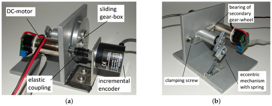
Figure 1.
A non-linear robotic mechanism: (a) front view, (b) back view.
2.1. Non-Linear, Single-Degree-of-Freedom Robotic Mechanism
Used robotic device (also non-linear robotic mechanism) is a single-degree-of-freedom mechanism that is simulated by an eccentric coupling with a spring to create a changeable and repetitive torque. It can be further partitioned into the following elements:
- DC-motor (ESCAP 28D11-219P) with a nominal voltage of , nominal current , nominal velocity rad/s, inertia moment × , viscous friction coefficient and nominal torque .
- Incremental encoder Omron E6B2-CWZ1Y of resolution 2000 pulses/rev (electronically multiplied by four to reach resolution 8000 pulses/rev), mechanically connected directly to the axis of the DC-motor using elastic coupling.
- Sliding gear-box with transmission ratio used to produce unexpected slips (unexpected load torque disturbances) between the primary and secondary axis of the sliding gear-box. The friction between both gear-wheels can be adjusted by a clamping screw which can move the bearing of the secondary gear-wheel left or right and thus adjust the amplitude of the slide between both gear-wheels. Maximum rotational velocity on the secondary side of the sliding gear-box is .
- The non-linear robotic mechanism with a spring used to drive the DC-motor from the motor to generator regime and vice versa, thus producing the repeatable load torque disturbances.
Repeatable load torque disturbances produced by the non-linear robotic mechanism with spring require that the DC-motor produces variable drive torque. The latter varies between the minimum and maximum torques, causing the DC-motor to switch to the generator regime and vice versa. When the secondary axis is rotated , the load torque reaches its maximum peak, and at the moment of rotation, the sliding gear-box usually slides between both contact surfaces. Furthermore, a singular point emerges between the minimum and maximum points when the drive torque is zero. The singular point is presented in Figure 2.
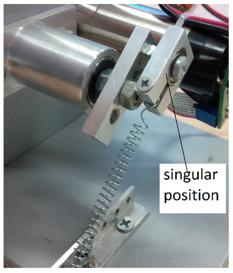
Figure 2.
A non-linear robotic mechanism: overview of singular position.
In the remainder of this section, we provide a detailed description of the controller, along with proof of non-linearity of the robotic mechanism.
2.2. Controller
The controller, illustrated in Figure 3, consists of a non-linear mechanism that is controlled by the inner current (faster) and outer velocity (slower) feedback controllers. Current control is designed using the linear PI-antiwindup controller with sampling time . The velocity controller runs at sampling time and can be implemented either as a classical PI-antiwindup or as the proposed OAC-DES controller, using a simple switch to select the desired mode. To guarantee equal conditions for both velocity controllers, the same sampling times are taken. Antiwindup controllers are used to prevent the integral (I element in PI-controller) windup that can cause sudden increases of a control variable and cause saturations of the non-linear robotic mechanism.
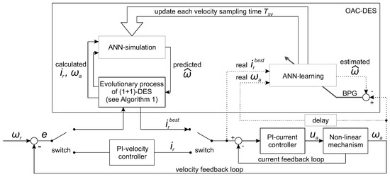
Figure 3.
Block scheme of controller with design of the OAC-DES.
As can be seen from Figure 3, design of the OAC-DES (presented in the upper rectangle) is more complex than the linear PI-controller, because of the coexistence of the (1+1)-DES and ANN. Although two ANNs are denoted in the OAC-DES box, i.e., ANN-learning and ANN-simulation, only a single ANN is used, although it plays two different roles. At first, ANN-learning is used to model the behavior of the estimated velocity according to the actual rotational velocity in real time. Next, the learned ANN is used to predict the velocity in the ANN-simulation needed for the calculation of the fitness function in (1+1)-DES. It is noteworthy that both phases, i.e., ANN-learning and (1+1)-DES are run sequentially one after another within one velocity sampling time . In each velocity sampling time , weights are updated according to the behavior of the control plant.
To prove that the control plant is really non-linear, a simple test was performed. Using the actual rotational velocity and reference current of a DC-motor , a non-linear characteristic was simultaneously recorded. The latter was varied within the interval A, and the actual rotational velocity was recorded. As a result, the double hysteresis-like curve of the non-linear characteristics was obtained, as shown in Figure 4.
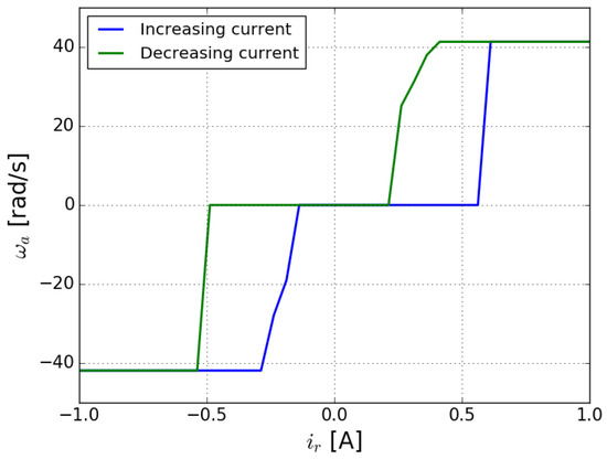
Figure 4.
Non-linear characteristic of the robotic mechanism.
Figure 4 shows the measured non-linear characteristic. First, when the reference current was increased, the DC-motor did not move due to the load of the spring. Next, when the reference current was increased still further, the DC-motor started to move, but did not rotate. By even further increasing the current, the DC-motor overcame the load at some point. As a consequence, the non-linear robotic mechanism started rotating at maximum velocity (the sudden jump of the blue line). Finally, additional increases in the reference current did not results in any further acceleration of the DC-motor.
Once rotating, the DC-motor did not react to slight decreases in the reference current. A significant decrease in was needed to reduce velocity, and two additional reference decreases were necessary to fully stop the DC-motor. Stopping the DC-motor was somewhat more gradual than starting it had been. The difference can be explained by static friction in the DC-motor and load, which is present only when starting the DC-motor.
2.3. Computer System with Power Electronics
A computer system with power electronics is both the brain and the heart of our application. A modern digital signal controller (DSC), together with a current sensor, are used as a computer system, while a motor driver and power supply unit (PSU) serve as power electronics. The former collects and processes necessary information, and enables execution of control algorithms. Actually, it is a hardware into which the (1+1)-DES is embedded. The latter delivers information received as a commands from the computer system to the DC-motor.
The following computer configuration is employed in our study:
- digital signal controller Texas Instruments TMS320F28377S Delfino,
- current sensor Allegro ACS712,
- motor driver STM L298N,
- power supply unit InterTech CombatPower CP-650W Plus.
The DSC architecture consists of two computer components: the central processing unit (CPU) and control law accelerator (CLA). These can both run on clock frequency 200 MHz in hardware parallelism and execute 800 million instructions per second (MIPS), which provides the means for the online execution of OAC-DES.
The control program is thus divided into two parts: the two linear controllers which run on the CLA accelerator (coprocessor), and the main management program, together with OAC-DES and ANN, which run on the CPU. Table 1 specifies the most important properties of TMS320F28377S [32].

Table 1.
Common characteristics of TMS320F28377S.
The current sensor operates on the Hall Effect. Its input is connected to the DC-motor, while the output goes to the DSC. It is then incorporated into the CPU using an A/D conversion. If the current sensor weakens the power of the DC-motor to receive usable information, then the motor driver does the opposite, i.e., strengthens the information to power the DC-motor. The PSU guarantees that the computer system and motor driver are well supplied.
3. Implementation of the OAC-DES
Many of the problems with which people are confronted today are dynamic in nature. This means that environmental conditions are not static, but change over time. In EAs, these changes often affect the real-time fitness function, whereby the optimal solution at one time is non-optimal at another and vice versa. Algorithms for solving dynamic problems must therefore [3]:
- be aware of the changing environment,
- respond to environmental changes efficiently.
Usually, the first condition can be met by using additional memory, where a redundant individual (also called a sentinel) is used in the population. The change in the fitness landscape is detected due to the change of the fitness function value. Indeed, the fitness value is changed after the environment has been changed. The prerequisite for the second condition is sufficient population diversity that allows the already converged population at the most recent optimum to search for the new optimum in a changed fitness landscape.
Classical EAs suffer from a lack of reactivity due to maintaining the population of the solution. Although this population allows EAs to find a near-optimum solution in many cases, the time needed for finding it is unsuitable for systems in real situations, in which the so-called feedback control systems must respond to a sequence of cause-and-effect relationships among the system variables. The theory of feedback control systems [33] asserts that for mechanical time constants of non-linear robotic mechanisms, a suitable sampling time should be between . This means that when the EAs are applied in the feedback control system, small populations with rapid responses should be achieved to limit the time complexity. Consequently, the most suitable EAs for this purpose are most certainly Evolution Strategies (ES) [34] that are, in their simplest configuration (1+1)-ES, capable of maintaining only one population member, and are therefore not too time complex. Additionally, ES also support self-adaptation, which is indispensible in achieving the fast response time of this feedback system.
Unfortunately, the (1+1)-ES cannot be run autonomously on the computer system, because of fitness function evaluation. This evaluation actually demands an immediate response from the feedback control system, where a behavior of the generated solution needs to be estimated. This means that the wrong solutions generated by (1+1)-DES could cause faulty operation of the control system, resulting in damage. At the same time, however, changing the test values of the real control system online is time consuming and therefore inappropriate for real-time processing. Therefore, in our study the evaluation is not performed on the real system directly, but is predicted using ANN-simulation.
However, reliable prediction by an ANN-simulator is possible only when it is conducted on the regularly learned ANN. Consequently, ANN-learning must be launched before ANN-simulation in each sampling time. The OAC-DES consists of three algorithms:
- ANN-learning,
- (1+1)-DES,
- ANN-simulation.
In the remainder of this paper, these OAC-DES algorithms are presented in detail.
3.1. ANN-Learning
ANNs are a universal tool for system modeling [35]. During the modeling, the ANN searches for an optimal mapping of the input to the output values. In our case, the main goal of the modeling is to incorporate the aforementioned non-linearity into the modeled system. This non-linearity is recognized during the ANN-learning process in which the proper ANN model is constructed on the basis of known pairs of input and output values. The learned ANN model is then capable of predicting output values according to the unknown input during the ANN-simulation.
The principle of ANN-learning, launched at the start of each sampling time before (1+1)-DES optimization, is presented in Figure 5, from which it can be seen that the ANN consists of two inputs, n-neurons in hidden layer “J”, and one neuron in output layer “L”. Linear activation functions are used for neurons in both the hidden and output layers [36]. The two inputs enter the ANN-learning block, i.e., the reference current and previous actual rotational velocity , while the output value returns the estimated rotational velocity , where k denotes the observed sampling time . In the feedback system, the supervisory back-propagation (BPG) learning algorithm is engaged for modifying the weights in the hidden and output layers. Thus, the BPG learning algorithm is guided by decreasing the magnitude of tracking error on the one hand, and the learning pace controlled by two learning rates, i.e., the hidden layer learning rate and output layer learning rate , on the other hand. The task of the BPG algorithm is to decrease the tracking error as much as possible.
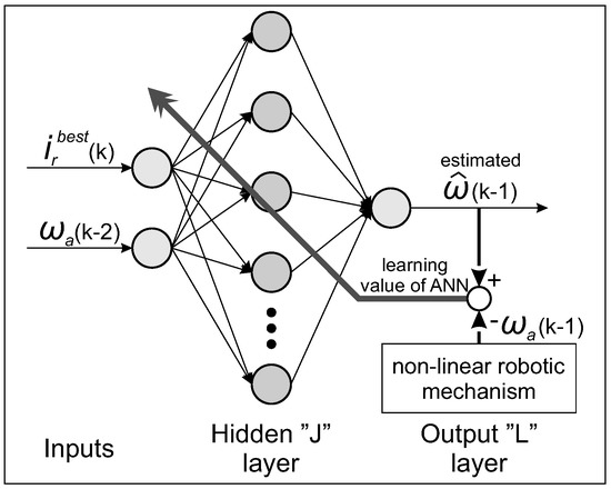
Figure 5.
Online ANN-learning.
Practically speaking, we realized that two simple rules apply with regard to BPG learning rates: (1) the higher the learning rates and , the more rapid the ANN-learning, and (2) divergence and instability may occur when the learning rates are set too high. Additionally, wrong starting weights may have a crucial influence on the stability of the system. Therefore, it is important to start the control process with proven weights found during so-called introductory ANN-learning, as described in detail below.
In summary, two diverse inputs in the ANN guarantee that it is equipped with enough information history for proper modeling. It is particularly important to keep the number of neurons in the input and hidden layers as low as possible. There are two reasons for this: (1) the learning process increases in complexity as the number of neurons increases, and consequently an extra time is needed for back-propagation, which is not suitable for real-time operation, and (2) the momentum problem occurs, whereby the ANN-simulation cannot predict the result properly due to low effect of the best reference current . By increasing the number of neurons, the variation of is lowered and therefore modeling becomes inaccurate. As a result, choosing the proper number of neurons in the hidden layer is crucial for system stability.
Introductory ANN-Learning
Introductory ANN-learning, or ANN-learning from scratch, usually takes a long time. Initial ANN weights are set using a random number generator. The purpose of introductory ANN-learning is to build a model based on the input/output pairs obtained from the control plant, which is good enough to be used as a stepping stone in the continuing operation of the OAC-DES. This learning should guarantee favorable starting weights of the ANN and thus prevent crashing of the OAC-DES controller. This is done by first running introductory ANN-learning until convergence occurs, and then storing the obtained weights in permanent memory. These then guarantee a stable and accurate start. However, this does not mean that ANN-learning cannot improve the weight values during OAC-DES operation. On the contrary, it only ensures that the controller does not crash instantly. The weights are then further improved during OAC-DES operation.
During introductory ANN-learning, the learning rates are lowered to the minimum in order to enable slow learning and to prevent instability of the non-linear robotic mechanism.
3.2. Evolutionary Algorithm in OAC-DES
In our study, the EA was moved from the disembodied computer system into real hardware in a dynamic environment, where it acts autonomously. In line with this, the fitness of solutions could not be calculated directly from a phenotype of solution, but had to be obtained after observation of how the phenotype reacted to the conditions of the dynamic process governed by the environment [37]. Thus, the behavior of the phenotype was evaluated after the solution was exposed to the dynamic conditions of the environment. Consequently, the traditional three-step evaluation chain genotype-phenotype-fitness was replaced by the four-step genotype-phenotype-behavior-fitness chain [29].
Moreover, evaluating the behavior of the solution in real-world systems presents another problem due to the need for long-term calculations. Therefore, a so-called surrogate model [29] was used to employ computationally cheaper models in place of full fitness function evaluations. As a result, in our study the behavior of the solution is predicted using ANN-simulation.
In what follows, the fundamentals of ES are discussed, after which the proposed (1+1)-DES algorithm is illustrated in detail.
3.2.1. Theory of ES
ES are especially suitable for solving global optimization, high-dimensional problems because of their insensitivity to becoming stuck in local optima. Normally, each individual in a population of solutions is represented as a real-valued vector:
where denotes the population size and n is a dimension of the problem to be solved.
The classical ES operates with a mutation only. As a mutation operator, a Gaussian perturbation is implemented. However, an uncorrelated mutation with one step size [38] was used in our study. This mutation requires expansion of the original representation of an individual with an additional control parameter , as follows:
where designates the mutation step size (also mutation strength). Actually, the individual is modified according to the following equations:
where represents a learning rate and is the random number drawn from the Gaussian distribution with mean zero and standard deviation one. To avoid falling too close to zero, the following boundary rule is used:
where is some predefined small value.
The mutation scheme represented in Equation (3) allows the process of self-adaptation, where the control parameters are included in the representation of individuals in Equation (2) and undergo the consequences of operating the mutation operator together with problem variables.
Normally, uniform random parent selection is used in ES, while two population models are typicaly employed, i.e., -ES and -ES. The first model generates offspring from a population of parents, from which the best offspring are preserved in the next population. In the second model, the offspring are generated from the population of parents that compete with their parents for a place in the next generation. A ratio between the number of generated offspring and parents of approximately , as found throughout most experimental work [34], is a prerequisite for successful self-adaptation.
Additionally, the evolutionary process can operate correctly in ESs only when a proper initial mutation step size is used. The proper range of step size values within which the search process can take place is called the evolution window. This, however, depends on the problem in question and must be determined during experimentation.
3.2.2. The Proposed (1+1)-DES
A characteristic of the feedback control system is that it responds to the desired input value (cause) with a measured output value (effect) such that the error tracking value becomes as small as possible. Thus, the response of the system must be instantaneous if we wish to build a purely reactive system. This assumption requires that the decision feedback response takes less than 5 ms. In our study, the decision-making process governing this response is entrusted to the single membered (1+1)-DES. Because we are dealing with a non-linear, single-degree-of-freedom robotic mechanism, we must solve the 1-dimensional optimization problem. Although the question may arise as to why EAs were used for solving such a seemingly trivial problem, it can be asserted that an increase in problem dimension would not have had a crucial influence on the performance of the proposed algorithm.
In each generation g, the proposed algorithm maintains two individuals and . The first individual denotes an evolution of the original solution, where the regular mutation step size normally decreases in each generation due to the multiplicative process in Equation (3), and thus allows smaller and smaller modifications of the problem variable . The second individual starts the evolution process using initial mutation step size in each generation anew, and thus allows for larger modifications of the problem variable . However, the better of the two individuals according to the fitness function is preserved in the new best solution .
The effect of using two different individuals in the (1+1)-DES is depicted in Figure 6, from which reactions of the algorithm to the hypothetical step signal can be viewed. Practically speaking, the modifiable regular step sizes are used to retain the current level (horizontal step signal) and to move the constant larger, initial ones to a higher/lower signal level (vertical step signal).
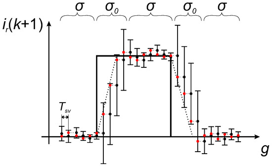
Figure 6.
Effect of the different mutation step sizes on optimization results.
In summary, the pseudocode of the proposed (1+1)-DES is illustrated in Algorithm 1, from which it can be seen that the proposed algorithm is launched at every sampling time using the following parameters: desired (reference) velocity , measured velocity , regular reference current and mutation step size , respectively. Actually, the last two parameters represent the starting point for the evolutionary search process. In each generation, two individuals and using different search strategies (i.e., different starting mutation step sizes) compete with each other to become the current best solution . Finally, the (1+1)-DES algorithm returns this best solution consisting of the best reference current and as optimized by the (1+1)-DES, and the best velocity as predicted by the ANN. Moreover, the best reference current is put on the control plant, and thus controls the velocity controller. Interestingly, the algorithm consists of two functions: (1) the ‘evaluation’ implementing Equation (5) and (2) the ‘mutation’ implementing Equation (3). We should emphasize that two fitness function evaluations are launched in each generation.
| Algorithm 1 Pseudocode of (1+1)-DES | |
| Input: Reference , measured , reference and . | |
| Local:, , and | |
| Output: The best reference , and . | |
| 1: | ; {initialization of an original solution} |
| 2: | ; {initialization of an initial solution} |
| 3: | ; {initialization of the best solution} |
| 4: | ; {current fitness} |
| 5: | fortodo |
| 6: | = mutate(); {uncorrelated mutation according to Equation (3)} |
| 7: | ; |
| 8: | = mutate(); {uncorrelated mutation according to Equation (3)} |
| 9: | ; |
| 10: | if then |
| 11: | |
| 12: | end if {long-step search prevailed?} |
| 13: | if then |
| 14: | |
| 15: | end if {best solution found} |
| 16: | end for |
| 17: | return; {the final solution: } |
3.3. ANN-Simulation
Fitness function evaluation is the most complex task in the (1+1)-DES, because the quality of the solution cannot be calculated directly, but must be determined by evaluating its behavior in real environmental conditions. Due to the time complexity of this estimation, the fitness evaluation is instead performed using ANN-simulation, which presents the surrogate model. In our study, the behavior of each solution is actually predicted using ANN-simulation as depicted in Figure 7, from which it can be seen that the same two inputs used in ANN-learning also enter into the ANN-simulation. The former is obtained from the non-linear robotic mechanism and denotes the measured velocity , while the latter shows the output from the (1+1)-DES and denotes the trial solution reference current (actually ), where determines whether either the original or the initial solution is evaluated, respectively. The output from the ANN-simulation presents the predicted velocity that enters into the fitness function calculation. This predicted value is then subtracted from a reference velocity (i.e., desired value), and the difference is squared to obtain the fitness function value. In other words, the fitness function is defined as:
where the square of the difference between the reference and predicted velocity ensures that the difference is always positive. The task of the (1+1)-DES is to minimize the value of the fitness function, with actual and reference velocities held constant during the single sample time interval.
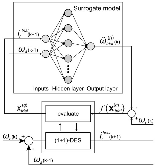
Figure 7.
The fitness function evaluation in OAC-DES.
4. Experiments and Results
The purpose of our experimental work was to show that the results of the proposed OAC-DES are comparable with (if not better than) the results of the linear PI-controller on the non-linear control plant. In line with this, several experiments were performed:
- proof of concept,
- real-time test,
- step response tests,
- influence of the spring constant.
In the first test, the OAC-DES and the linear PI-controller were compared according to the error between the desired and actual values of the rotational velocity in order to show that the former is capable of adapting, in contrast to the latter. The purpose of the real-time test was to show that the time complexities of the OAC-DES components allow for its online response (i.e., reacting in less than 5 ms). In the next experiment, step responses of the OAC-DES, obtained in different tests, were compared to the responses of the linear PI-controller on the same step function. The last experiment highlights the influence of the spring constant k. Indeed, the step response tests were measured at two reference velocities: and .
For all tests, initialization of the OAC-DES was performed using weights as found after the introductory ANN-learning phase. However, these alone do not guarantee controller stability, and therefore, a reduced introductory ANN-learning was conducted on input/output pairs obtained by the linear PI-controller with a duration of T = 0.5 s before each OAC-DES startup. The purpose of this procedure was twofold: (1) to avoid the need for ANN-learning from scratch, which lasts about 12–15 min, and (2) to ensure that ANN-learning is adapted to current control loop demands prior OAC-DES operation.
During the experiments, the same velocity and current feedback loops were used in order to compare both observed velocity controllers as fairly as possible. The linear current PI- and velocity PI-controllers were tuned manually using the Ziegler-Nichols method [39], which is a popular method of tuning the parameters of linear PI-controllers with a linear control plant. The PI-controller parameters thus obtained were then changed slightly to adapt them to the non-linear plant. On the other hand, the proposed OAC-DES controls the velocity controller automatically [23].
The current controller constants as presented in Table 2 were set equally for both of the velocity controllers in the tests.

Table 2.
Linear current PI- and linear velocity PI-controllers constants.
Table 3 specifies the topology of the ANN used by the OAC-DES.

Table 3.
Topology of the ANN.
We should mention that the proper topology was obtained after extensive testing. Moreover, the BPG algorithm was run at exactly = 20 epochs, while both the learning rates were set as during the control process.
The parameter setup of the (1+1)-DES used during the experiments is presented in Table 4, from which it can be seen that the initial reference current value was set to A and the maximum reference current to . For a short time, actual current may exceed maximum reference current. The (1+1)-DES terminates, when the maximum number of generations is reached.

Table 4.
Parameter setup of (1+1)-DES.
In the remainder of the paper, the experiments are described in detail.
4.1. Proof of Concept
In this verification test (also called proof of concept), we compare the performances of both controllers used in our study, i.e., the OAC-DES and linear PI-controller, according to a Root Mean Squared Error (RMSE) indicator. The RMSE indicator is frequently used in control theory for measuring the quality of a control system, where the difference between desired and actual values is observed. The lower the RMSE value, the better the response of the control system. Using this test, we would like to reveal the adaptive nature of the OAC-DES during online control that is its major advance over the linear PI-controller.
The RMSE indicator is expressed as follows:
where N represents the number of samples (every velocity sampling time = 3 ms) in one cycle of duration .
Using the RMSE indicator, the test was conducted similarly for both controllers. At first, the reference generator for velocity control for duration acts as a repeatable driving cycle. For each velocity sampling time , the squared difference between reference and actual velocity is calculated. The differences are then summed up for the duration of the whole cycle . For instance, there are approximately samples, when s, and samples, when s. The driving cycle is depicted in detail in Section 4.3.1.
The results of the comparison between OAC-DES and linear PI-controller during the proof of concept test are shown in Figure 8, where the behavior of the OAC-DES with ANN-learning is compared with the behavior of the linear PI-controller without learning. The figure shows that at the beginning, the linear PI-controller controls the non-linear robotic mechanism more effectively. However, the RMSE indicator for the linear PI-controller remains constant, while it decreases significantly for the OAC-DES during online control, and in fact becomes equal to the linear PI-controller after 5 cycles (i.e., 22.5 s). Furthermore, when the introductory ANN-learning continues, the RMSE indicator decreases steeply for the OAC-DES up to the 11-th cycle, when it starts to decrease gradually.
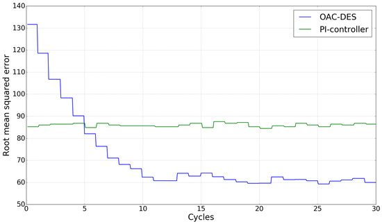
Figure 8.
Online control RMSE comparison between linear PI-controller and OAC-DES.
According to Figure 8, the behavior of the linear PI-controller is much better than that of the OAC-DES during earlier cycles, but falls very far behind after. Obviously, for optimal control, the OAC-DES requires some time to recognize the non-linearity of the system more precisely. This is the crucial limitation, and should be taken into account for the tests that follow.
4.2. Real-Time Test
The purpose of this experiment was to show that the real-time complexity of the proposed OAC-DES is less than the requested velocity sampling time . Indeed, three program routines running consecutively one after another increased the response time of the adaptive controller. The first routine was dedicated to measuring the rotational velocity , the second to ANN-learning, and the third to executing the (1+1)-DES optimization algorithm.
The partial time complexity of each routine was measured using a Tektronix TBS1052B digital oscilloscope. Obviously, the total time complexity of the proposed controller was obtained simply by adding together the individual time complexities of all three program routines. In fact, the velocity sampling time was determined on the basis of the measured total time complexity, which consequently ensured there would be enough time for the successful execution of all three routines. On the other hand, the OAC-DES responds in real-time when the velocity sampling time is drawn from the interval ms.
The results of the real-time test are illustrated in Figure 9, where the real-time execution of the OAC-DES is presented.

Figure 9.
Real-time complexity estimation.
As can be seen in the figure, ANN-learning took 560 s on average. The online learning and evaluation never took the same amount of time. More precisely, the minimum ANN-learning time was 540 s, while the maximum was 600 s. On the other hand, the execution of the (1+1)-DES using 10 generations (21 evaluations of ANN-simulation) lasted 650 s on average, where the single evaluation of the fitness function using the ANN-simulation went on for 8.3 s. More precisely, the minimal time complexity of the (1+1)-DES was 640 s, while the maximum was 690 s. As a result, ANN-learning and (1+1)-DES optimization together took ms on average, which means that enough time was left for applying more complex nature-inspired algorithms in the future.
In contrast, we neglected the time complexity of linear PI-controllers due to their simplicity and rapid execution on the CLA coprocessor. Furthermore, the program routine for this controller was written in the assembly language, which ensures that execution takes less than 10 s.
4.3. Step Response Tests
The performance of the proposed OAC-DES was evaluated by extensive empirical testing. For the non-linear robotic mechanism, we specified a sequence of desired signals (driving cycle), which act as velocity control references . In line with this, the non-linear robotic mechanism’s reactions were recorded according to the actual velocity on the oscilloscope. These reactions are known as velocity control responses. The closer the step response to velocity control reference, the better the controller.
In our study, we were actually interested in the results of three step response tests:
- the reaction of the actual velocity to the changing reference velocity (velocity control response),
- the difference between the actual and reference velocities obtained by changing the output of the velocity controller,
- the output from the particular velocity controller in the form of a reference current signal .
We should mention that the first step response primarily estimates the performance of the controller.
As such, two separate tests were conducted. The purpose of the first was to test robotic behavior on the control plant using the reference velocity , while the second used the higher reference velocity . During experimentation, the actual velocity control response, velocity error, and reference current (i.e., output of OAC-DES) were measured.
Normally, the response of the feedback system to the step function consists of overshoot and consequential settling. Additionally, in our case, periodic disturbances were experienced by the system due to the load torque caused by spring. In control theory, both signals present so-called peak errors, which are divided into two types:
- transient peaks: error peaks due to transient responses immediately after overshooting,
- disturbance peaks: steady state error peaks due to load torque perturbations.
In the remainder of the paper, these step response tests are described in detail.
4.3.1. Step Response Tests at Reference Velocity 10 rad/s
In the first experiment, a comparison between the linear velocity PI-controller and proposed OAC-DES controller was conducted according to the three previously mentioned step responses. These responses are depicted in Figure 10, which is divided into two diagrams denoted as Figure 10a,b. The former presents the step responses of the linear PI-controller, the latter those of the OAC-DES. Each diagram consists of three graphs depicting the corresponding step responses numbered from 1 to 3, respectively.
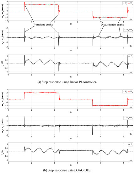
Figure 10.
Step response at reference velocity .
The graphs for the step response 1 show improvements of the OAC-DES compared to the linear PI-controller according to the velocity feedback loop. As can be seen in Figure 10, the overshoot, denoted as a transient peak in the figure representing the linear PI-controller, is much higher than for the OAC-DES. The former amounts to 40% of the whole step signal, while the latter is only 10%.
The graphs for the step response 2 show much higher disturbance peaks for the linear PI-controller than for the OAC-DES. This means that the linear PI-controller initiates a periodic perturbations cannot be eliminated, while the OAC-DES adapts to the oscillations and eliminates the steady state errors almost perfectly.
Interestingly, neither controller had any problem controlling steady state error when the reference value was , although the response of the OAC-DES was a bit more restless.
The graphs illustrating step response 3 are very important, as they directly react to velocity error and therefore dictate the actual velocity . When promptness of the reactions is compared, we find that the linear PI-controller reacts more quickly and intensively, and consequently obtains a higher overshoot. The current ripples for this controller are almost twice as high as those of the OAC-DES. On the other hand, the OAC-DES reacts more prudently and therefore causes less stress on the non-linear robotic mechanism. This is reflected in the reduced reference current ripples and reduced transient peaks. Although the OAC-DES does have advantages compared to the linear PI-controller, the high-frequency noise has been caused by reference current when using the OAC-DES, especially at .
4.3.2. Step Response Tests at Reference Velocity 30 rad/s
In this experiment, we compared the linear velocity PI-controller and the OAC-DES at reference velocity . The results of the comparison are illustrated in Figure 11, which is organized in the same way as in the last subsection. Therefore, we focus our discussion here on the results according to the three step responses presented in the corresponding graphs.
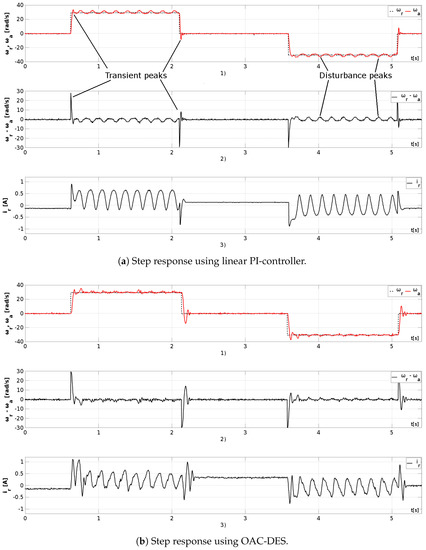
Figure 11.
Step response at reference velocity .
Step response 1 graphs show similar transient reactions of the linear PI-controller and the OAC-DES. Since velocities are higher, overshoots are recognized by both of them. However, transient peaks, just like the disturbance peaks, are a bit higher in the case of the OAC-DES. More precisely, these range up to 6 rad/s for the OAC-DEC, compared to 4 rad/s for the linear PI-controller. It is important to note that the disturbance peaks of OAC-DES lower due to adaptation, while these remain constant in the case of the linear PI-controller. The reason for the raised disturbance peaks lies in the increased velocity, which increases the number of disturbances per time unit. Thus, the OAC-DES reacts a bit slower and additionally becomes more restless when reference velocity .
Despite those facts, it seems that the OAC-DES is the better controller even in this case, because it can adapt to arbitrary disturbances. The more disturbances there are, the more “experienced” the OAC-DES becomes. As the graph for step response 2 shows, soon after the transient peak emerged during the change from to , the disturbance hit the non-linear robotic mechanism, resulting in the disturbance peak. The velocity error of the actual velocity according to reference velocity becomes noticeable. The first disturbance peak is usually the highest of all peaks in the series. The OAC-DES sequentially adapts to those peaks, and each subsequent error is slightly reduced. The sixth disturbance in the series unexpectedly diverges slightly from the OAC-DES, and the adaptation process repeats.
Another example of adaptation can be seen in the transient response when the reference velocity is changed from to . The transient peak is the highest in the series. Then, a bit lower, the first disturbance peak follows, after which all subsequent disturbance peaks are progressively lower. Indeed, we conclude from this that the proposed OAC-DES controller is capable of reducing periodic disturbances in both directions.
In the graph of step response 3, the output variable for the linear PI-controller indicates equivalent reactions to each disturbance. On the other hand, the OAC-DES does not react to each disturbance in the same way, but rather changes both the shape and the magnitude of the reactions. This further supports its adaptation to disturbances. However, reactions to transients are one of the bottlenecks associated with the proposed OAC-DES, since the reference current becomes uncertain within these regions.
4.4. Influence of the Spring Constant
In the last experiment, an influence of a spring constant k was taken into consideration. According to the Hook’s law, the spring constant determines the size of deformation by force loading. The higher the force, the higher the deformation of the elastic body (e.g., spring). Thus, it is expected that the higher spring constants would deteriorate the performance of both used controllers. In line with this, the responses of the controllers by controlling the non-linear robotic mechanism loaded with springs of three various constants were applied in our experiments: N/m, N/m, and N/m. However, in the previous experiment, where the step responses at reference velocity rad/s and rad/s were observed, the spring with constant N/m was used. As a result, in this test, these results need to be supplemented with the results obtained by both controllers when the non-linear robotic mechanism was loaded with springs of constants N/m and N/m.
As can be shown in Figure 12, it becomes more difficult for a DC-motor to overcome the load by tightening springs, or increasing the spring constant. Hence, reference current significantly increases and occasionally hits the maximum reference current (). This means, transient peaks increase for linear PI-controller, while the same decrease for OAC-DES. The same finding applies also for disturbance peaks: these increase for the linear PI-controller and the same ones roughly decrease, or stay unchanged for the OAC-DES. The quality of the proposed controller and its benefit thus come into play at higher loads. However, a significant deterioration is observed for the OAC-DES in case of reference velocity . Compared to Figure 10, the OAC-DES restlessness undoubtedly increases. Restlessness most clearly becomes observable at current reference step response and it is expected, that it will even worsen by further tightening the load. Linear PI-controller on the other hand constitutes smooth current reference , which treats the DC-motor more generously—does not cause instantaneous changes, and thus lower the restlessness. Despite this fact, linear PI-controller velocity step responses become unacceptable for a decent use in practice.
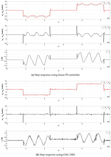
Figure 12.
Step response at reference velocity , spring constant N/m.
Figure 13 depicts controllers step responses, when the spring constant is set at N/m, which makes the DC-motor difficult to overcome the load. Therefore, the reference current becomes regularly saturated at maximum actual current (). This fact causes the following phenomenon: when the spring is loaded at its peak, actual velocity automatically drops and cannot attain the reference velocity . Phenomenon is not caused by controller itself and thus cannot be eliminated easily; the limited actual current should be increased to avoid it, but this might harm existing DC-motor, which should be replaced with a larger one in that case.
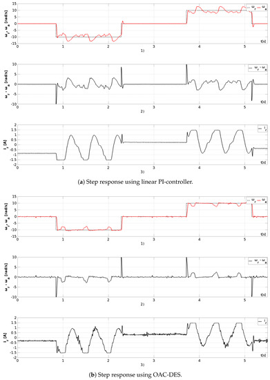
Figure 13.
Step response at reference velocity , spring constant N/m.
As expected, by introducing the heaviest load, disturbance peaks for linear PI-controller become even worse, while transient peaks become partially eliminated. For the OAC-DES, velocity step response becomes occasionally biased due to the reference current saturation, but it exhibits a reliable performance otherwise. Again, reference current restlessness becomes noticeable for the OAC-DES.
4.5. Discussion
Using the laboratory setup, we successfully implemented a real-time online controller that uses ANN for modeling and ES for optimization. We have offered the real-time analysis and proved the convergence of the proposed controller. Additionally, we have shown that under certain conditions, the OAC-DES undoubtedly exceeds the capacities of the linear PI-controller.
In general, we conclude from the results of the step response tests that the OAC-DES reacts to the changes of the step function comparable, or better than the linear PI-controller does. At lower velocities, it achieves lower transient peaks (overshoots). Since it can adapt to disturbance peaks, the OAC-DES also reduces them during the adaptation and over time may even eliminate them altogether. Unfortunately, problems occur due to the noisy reference current and actual velocity . Thus, the OAC-DES increases steady state error, since it appears that the ANN needs constant velocity excitements to work properly.
At higher velocities, the OAC-DES slightly under-performs the linear PI-controller. Transient peaks increase and promptness declines. However, it adapts to disturbances of the non-linear robotic mechanism, resulting in a reduction in a steady state error. This indicates that the OAC-DES has not yet adapted optimally to control plant and requires additional learning time. Indeed, we have discovered that, as long as the step reference is below , the OAC-DES produces negligible disturbance peaks which start to rise only when the step reference exceeds . Nevertheless, for common robotic applications, actual velocities on the secondary axis of up are easily sufficient.
We observed, that spring load heavily affects the linear PI-controller as follows: it becomes less and less manageable by increasing the load. Step responses might be acceptable for a wider practice only at the lowest spring constant N/m. Performance of the OAC-DES, on the other hand, does not deteriorate much by increasing the spring load (not taking the reference current saturation into account), but restlessness becomes very disturbing.
During testing, there were two periodic occasions: periodic disturbances and periodic control cycle. Therefore, two types of adaptation appeared: (1) adaptation to the periodic disturbances, or short-term adaptation, and (2) adaptation to the periodic control cycle, or long-term adaptation.
The first is valid for a single reference velocity, e.g., for one series , while the second comes into play when adaptations from the previous cycle are carried over to the next one. However, the OAC-DES requires time to adapt, and the longer the adaptation time the better the step response (Figure 8). This means that, given sufficient time, the OAC-DES will control the non-linear robotic mechanism optimally.
5. Conclusions
In general, EAs are stochastic, population-based, nature-inspired algorithms that have long been considered too time complex for solving dynamic problems. This paper tries to refute this myth by proposing an online adaptive controller based on the (1+1)-DES algorithm. The (1+1)-DES uses single-membered population that reduces time complexity on the one hand, while exploiting an inherent feature of ES, i.e., the self-adaptation, on the other. This feature allows the proposed algorithm to track the continuous changes in the input variable of the controlled system precisely, due to the mutation operator’s likely preference for smaller changes over larger ones.
The experimental results of the proposed OAC-DES show fairly better properties in comparison with a linear PI-controller for the same highly non-linear plant and sampling time ms. The ability to lower transient and disturbance peaks, reduce steady state error in the step responses of the velocity feedback control loop, and to offer online adaptation capability to load torque changes and unexpected torque disturbances, makes the OAC-DES an excellent candidate to control of fast mechatronic devices such as a non-linear, single-degree-of-freedom robotic mechanism. The rapid response time of the proposed OAC-DES in adapting to torque disturbances could also be further increased simply by adding more evaluations in the (1+1)-DES algorithm.
The unique advantages of using the (1+1)-DES algorithm in the OAC-DES include:
- It is simple to perform complete optimization within 10 generations within the sampling time of the feedback-controlled system ms.
- It can avoid being stuck at into local minimum in the way comparable adaptive online control methods based on gradient learning algorithms (e.g., ANN or classical least square methods) often are. A detailed proof of global convergence for (1+1)-ES with constant mutation strength is found in [40].
These results suggest that properly developed and tuned EAs could also be used in online environments, where robustness and rapid response are the most important requirements. From this we conclude that this controller has great potential for future development. This development could take several directions, but in general this type of controller would be most suitable for constantly changeable and unpredictable control plants, as for instance: (1) a direct-drive robotic mechanism with more degrees of freedom could be used, or (2) the same algorithm could be applied in other feedback control systems (e.g., for adaptive cruise control in automotive industry, or control of hydraulic cylinders and motors). Nevertheless, other population-based, nature-inspired algorithms could be incorporated into the OAC-DES and tested on the non-linear robotic mechanism. Also, a theoretic analysis of the OAC-DES rigorous system’s stability is an important task left for the future.
In our opinion, the proposed approach could be generalized from a single order dynamic system to higher order dynamic systems. However, serious problems with initial introductory learning may be encountered during the start-up, and thus a step-by-step process should be employed. In line with this, step wise learning is proposed here, where controlling the simplest axis would be learned first, followed by the next axis, and so on. For the purposes of higher order dynamic systems, a faster computer configuration would be needed, and the program code of the (1+1)-DES algorithm would need to be time-optimized. Nevertheless, restlessness of OAC-DES should be taken into account and proper remediation should be implemented.
Author Contributions
Methodology, R.Š., D.F. and I.F.; Software, D.F.; Validation, J.Š., I.F.J., I.F., R.Š. and D.F.; Writing—original draft, R.Š., D.F., J.Š., I.F.J. and I.F.; Data curation, I.F.J.
Funding
This research received no external funding.
Acknowledgments
Iztok Fister Jr. acknowledges the financial support from the Slovenian Research Agency (Research Core Funding No. P2-0057). Iztok Fister acknowledges the financial support from the Slovenian Research Agency (Research Core Funding No. P2-0041).
Conflicts of Interest
The authors declare no conflict of interest.
References
- Garey, M.R.; Johnson, D.S. Computers and Intractability: A Guide to the Theory of NP-Completeness; W. H. Freeman & Co.: New York, NY, USA, 1979. [Google Scholar]
- Darwin, C. On the Origin of Species; Harvard University Press: London, UK, 1852. [Google Scholar]
- Morrison, R.W. Designing Evolutionary Algorithms for Dynamic Environments; Springer: Berlin/Heidelberg, Germany, 2004. [Google Scholar]
- Stadler, P.F. Fitness landscapes. In Lecture Notes in Physics; Springer: Berlin/Heidelberg, Germany, 2002; pp. 183–204. [Google Scholar]
- Williams, K.R. Applications of Genetic Algorithms to a Variety of Problems in Physics and Astronomy. Master’s Thesis, University of Tennessee, Knoxville, IL, USA, 2005. [Google Scholar]
- Gutierrez, J.A.G.; Cotta, C.; Fernandez-Leiva, A.J. Evolutionary Computation in Astronomy and Astrophysics: A Review. arXiv, 2012; arXiv:1202.2523. [Google Scholar]
- Bäck, T. On the behavior of evolutionary algorithms in dynamic environments. In Proceedings of the 1998 IEEE International Conference on Evolutionary Computation, IEEE World Congress on Computational Intelligence (Cat. No. 98TH8360), Anchorage, AK, USA, 4–9 May 1998; pp. 446–451. [Google Scholar] [CrossRef]
- Müller, N.; Glasmachers, T. Challenges in High-dimensional Reinforcement Learning with Evolution Strategies. arXiv, 2018; arXiv:1806.01224. [Google Scholar]
- Andrés-Pérez, E.; González-Juárez, D.; Martin-Burgos, M.J.; Carro-Calvo, L. Constrained Single-Point Aerodynamic Shape Optimization of the DPW-W1 Wing Through Evolutionary Programming and Support Vector Machines. In Advances in Evolutionary and Deterministic Methods for Design, Optimization and Control in Engineering and Sciences; Springer: Berlin/Heidelberg, Germany, 2018; pp. 35–48. [Google Scholar]
- Wei, L.W.; Li, W.W.; Zhang, Y.; Qiang, X. A New Method Evaluating Credit Risk with ES Based LS-SVM-MK. In DEStech Transactions on Computer Science and Engineering; DEStech Publications, Inc.: Lancaster, PA, USA, 2017. [Google Scholar]
- Simões, A.; Costa, E. Prediction in Evolutionary Algorithms for Dynamic Environments Using Markov Chains and Nonlinear Regression. In Proceedings of the 11th Annual Conference on Genetic and Evolutionary Computation, Montreal, QC, Canada, 8–12 July 2009; ACM: New York, NY, USA, 2009; pp. 883–890. [Google Scholar] [CrossRef]
- Richter, H. Evolutionary optimization and dynamic fitness landscapes. In Evolutionary Algorithms and Chaotic Systems; Springer: Berlin/Heidelberg, Germany, 2010; pp. 409–446. [Google Scholar]
- Hughes, M. Investigating the effects Diversity Mechanisms have on Evolutionary Algorithms in Dynamic Environments. arXiv, 2016; arXiv:1610.02732. [Google Scholar]
- Vlasov, A.; Fedorenko, V.; Yakovlev, V. Application of the Evolutionary Algorithm for Creating Advanced Technologies for the Beneficial Use of Gas in Order to Increase the Efficiency and Reliability of the Operation of the Technological Equipment. In Proceedings of the SPE Russian Petroleum Technology Conference, Moscow, Russia, 15–17 October 2018. [Google Scholar]
- Brest, J.; Zamuda, A.; Boškovič, B.; Maučec, M.S.; Žumer, V. Dynamic optimization using Self-Adaptive Differential Evolution. In Proceedings of the 2009 IEEE Congress on Evolutionary Computation, Trondheim, Norway, 18–21 May 2009; pp. 415–422. [Google Scholar]
- Das, S.; Mandal, A.; Mukherjee, R. An Adaptive Differential Evolution Algorithm for Global Optimization in Dynamic Environments. IEEE Trans. Cybern. 2014, 44, 966–978. [Google Scholar] [CrossRef] [PubMed]
- Rodríguez-Molina, A.; Villarreal-Cervantes, M.G.; Aldape-Pérez, M. An adaptive control study for a DC motor using meta-heuristic algorithms. IFAC-PapersOnLine 2017, 50, 13114–13120. [Google Scholar] [CrossRef]
- Chmiel, W.; Kwiecień, J. Quantum-Inspired Evolutionary Approach for the Quadratic Assignment Problem. Entropy 2018, 20, 781. [Google Scholar] [CrossRef]
- Cruz, C.; González, J.R.; Pelta, D.A. Optimization in dynamic environments: A survey on problems, methods and measures. Soft Comput. 2011, 15, 1427–1448. [Google Scholar] [CrossRef]
- Nguyen, T.T.; Yang, S.; Branke, J. Evolutionary dynamic optimization: A survey of the state of the art. Swarm Evol. Comput. 2012, 6, 1–24. [Google Scholar] [CrossRef]
- Caleffi, M.; Akyildiz, I.; Paura, L. On the Solution of the Steiner Tree NP-Hard Problem via Physarum BioNetwork. IEEE/ACM Trans. Netw. 2015, 23, 1092–1106. [Google Scholar] [CrossRef]
- Caleffi, M.; Trianni, V.; Cacciapuoti, A. Self-Organizing Strategy Design for Heterogeneous Coexistence in the Sub-6 GHz. IEEE Trans. Wirel. Commun. 2018. [Google Scholar] [CrossRef]
- Fister, D.; Fister, I.J.; Fister, I.; Šafarič, R. Parameter tuning of PID controller with reactive nature-inspired algorithms. Robot. Autom. Syst. 2016, 84, 64–75. [Google Scholar] [CrossRef]
- Jezernik, K.; Rodič, M.; Šafarič, R.; Curk, B. Neural network sliding mode robot control. Robotica 1997, 15, 23–30. [Google Scholar] [CrossRef]
- Šafarič, R.; Jezernik, K.; Pec, M. Neural network control for direct-drive robot mechanisms. Eng. Appl. Artif. Intell. 1998, 6, 735–745. [Google Scholar] [CrossRef]
- Rechenberg, I. Evolutionsstrategie: Optimierung Technischer Systeme nach Prinzipien der Biologischen Evolution; Problemata Frommann-Holzboog: Stuttgart, Germany, 1973. [Google Scholar]
- Schwefel, H.P. Numerische Optimierung von Computer-Modellen Mittels der Evolutionsstrategie: Mit Einer Vergleichenden Einführung in die Hill-Climbing- und Zufallsstrategie; Interdisciplinary Systems Research; Birkhäuser Basel: Basel, Switzerland, 1976. [Google Scholar]
- Doncieux, S.; Mouret, J.B. Beyond black-box optimization: A review of selective pressures for evolutionary robotics. Evol. Intell. 2014, 7, 71–93. [Google Scholar] [CrossRef]
- Eiben, A.E.; Smith, J.E. From evolutionary computation to the evolution of things. Nature 2015, 521, 476–482. [Google Scholar] [CrossRef] [PubMed]
- Russell, S.; Norvig, P. Artificial Intelligence: A Modern Approach; Prentice Hall: Upper Saddle River, NJ, USA, 2009. [Google Scholar]
- Lopez-Garcia, P.; Onieva, E.; Osaba, E.; Masegosa, A.D.; Perallos, A. A hybrid method for short-term traffic congestion forecasting using genetic algorithms and cross entropy. IEEE Trans. Intell. Transp. Syst. 2016, 17, 557–569. [Google Scholar] [CrossRef]
- Texas, I. TMS320F2837xS Delfino Microcontrollers; Texas Instruments: Dallas, TX, USA, 2015. [Google Scholar]
- Uran, S.; Šafarič, R. Neural-network estimation of the variable plant for adaptive sliding-mode controller. Strojniški Vestn.-J. Mech. Eng. 2012, 58, 93–101. [Google Scholar] [CrossRef]
- Bäck, T. Evolutionary Algorithms in Theory and Practice: Evolution Strategies, Evolutionary Programming, Genetic Algorithms; Oxford University Press: Oxford, UK, 1996. [Google Scholar]
- Demuth, H.B.; Beale, M.H.; De Jesús, O.; Hagan, M.T. Neural Network Design, 2nd ed.; Martin Hagan: Jersey City, NJ, USA, 2014. [Google Scholar]
- Engelbrecht, A.P. Computational Intelligence: An Introduction; John Wiley & Sons: Chichester, UK, 2007. [Google Scholar]
- Fister, I.; Iglesias, A.; Galvez, A.; Del Sser, J.; Osaba, E.; Fister, I., Jr. Using novelty search in differential evolution. In International Conference on Practical Applications of Agents and Multi-Agent Systems; Communications in Computer and Information Science; Springer: Cham, Switzerland, 2018; pp. 534–542. [Google Scholar] [CrossRef]
- Eiben, A.E.; Smith, J.E. Introduction to Evolutionary Computing, 2nd ed.; Springer: Berlin/Heidelberg, Germany, 2015. [Google Scholar]
- Ziegler, J.G.; Nichols, N.B. Optimum settings for automatic controllers. Trans. ASME 1942, 64, 759–768. [Google Scholar] [CrossRef]
- Beyer, H.G. Theory of Evolution Strategies; Springer: Berlin/Heidelberg, Germany, 2001. [Google Scholar]
© 2018 by the authors. Licensee MDPI, Basel, Switzerland. This article is an open access article distributed under the terms and conditions of the Creative Commons Attribution (CC BY) license (http://creativecommons.org/licenses/by/4.0/).