Differential Learning for Outliers: A Case Study of Water Demand Prediction

Featured Application

Prediction of daily water demands.

Abstract

Predicting water demands is becoming increasingly critical because of the scarcity of this natural resource. In fact, the subject was the focus of numerous studies by a large number of researchers around the world. Several models have been proposed that are able to predict water demands using both statistical and machine learning techniques. These models have successfully identified features that can impact water demand trends for rural and metropolitan areas. However, while the above models, including recurrent network models proposed by the authors are able to predict normal water demands, most have difficulty estimating potential deviations from the norms. Outliers in water demand can be due to various reasons including high temperatures and voluntary or mandatory consumption restrictions by the water utility companies. Estimating these deviations is necessary, especially for water utility companies with a small service footprint, in order to efficiently plan water distribution. This paper proposes a differential learning model that can help model both over-consumption and under-consumption. The proposed differential model builds on a previously proposed recurrent neural network model that was successfully used to predict water demand in central Indiana.

1. Introduction

Accurate water consumption prediction models provide city planners with information to support infrastructure design and city planning. Water utility companies also use these models to optimize operations. In general, long-term prediction models are used for planning while short-term daily and monthly prediction models are used for operational decision support. Utility companies maintain these models over time and adjust them based on predicted weather conditions as well as changes in their service areas.

In a previous study [1], we developed a daily prediction model based on recurrent neural networks for water demand in central Indiana. This model was compared to two other models based on multiple linear regression and feed-forward neural network. All three models were trained using data from 1997 to 2010 and then tested over a period of five years from 2011 to 2015. The average error over the testing period was 12.73% for the multiple linear regression model, 8.84% for the feed-forward neural network and 3.84% for the recurrent neural network.

The recurrent network model yielded the highest predictive accuracy. Each input feature in this model was analyzed in order to reduce the number of features in the model while retaining its high accuracy. The initial recurrent network model included the following features: day of the year, holiday, maximum temperature, minimum temperature, rainfall, snow, snow depth, number of customers and average income. The revised recurrent network model included fewer features which consisted of day of the year, maximum temperature and precipitation as the sum of rainfall and snow. This latter model resulted in an average error of 3.17% over the testing period from 2011 to 2015.

While the above low average errors are indicative of the highly predictive nature of the recurrent neural network model, it was observed that most of the errors were associated with outliers days that had unexpected low or high water demands [1].

In this paper, we propose an enhanced model that can provide utility companies with estimated ranges for water demands in the case of over-consumption or under-consumption. This new model does not considerably improve the prediction error for normal water demand days however, it does provide lower and upper bound estimates for water demand during outlier days. The proposed model consists of three parallel networks:

• Baseline network for normal days,
• Positive outlier network for over-consumption days and
• Negative outlier network for under-consumption days.

Predicting water demand for outlier days is difficult because of the limited number of occurrences of these days even over an extended historical period. The aim of the proposed model is to provide a range for the expected daily water demand as well as the potential deviation from normal consumption levels. Section 2 of this paper summarizes previous related work. Section 3 describes the water demand data set used in this study. Section 4 discusses the performance of the daily water demand models and their limitations especially in the case of outlier days. Section 5 introduces the new differential learning network and investigates various training methods for the proposed model. Section 6 summarizes the findings of this paper and offers direction for future work.

2. Related Work

Predicting water demand has been an active area of research for several decades. This interest is motivated by the increase in water consumption as a result of urbanization as well as the limited availability of this natural resource. A review of various water demand modeling approaches over the last three decades is provided in [2]. This review highlights the differences between short-term and long-term predictions. In general, the focus of previous research in this area is either on identifying predictive features or developing predictive models for water demand.

With respect to predictive features, the correlation between water consumption and weather conditions was confirmed in [1,3,4,5]. In particular, temperature and precipitation have been identified as having a strong influence on water demand. Temperature and rainfall were used in [3]. Temperature and precipitation were used in [4]. In [6], a water demand prediction model for summer using maximum temperature, holiday and previous day’s water demand was proposed.

Economic factors such as water price and household income were also identified as key features in water demand prediction in [2]. An analysis of the spatio-temporal patterns of water consumption across the United States [7] concluded that urban areas are more efficient in terms of water usage. Higher efficiency of water usage was also observed in counties with higher income and education levels.

Different models were also proposed for water demand prediction. These include regression, time-series clustering, support vector regression and neural networks. In [3,4], linear regression models were used. Seasonal variations in hourly and daily water demand patterns are investigated in [8,9]. In [8], time-series clustering and support vector regression (SVR) were used for hourly water demand prediction in Milan, Italy. Patterns for the type of day (e.g., weekday, weekend or holiday) and specific periods of the year (e.g., spring, summer, fall or winter) were identified. The water supplied up to 6 a.m. in the morning was then used to generate an accurate prediction for water demand for the rest of the day. Different SVRs were trained for each hour of the day and for each pattern. The resulting model was able to predict within a 2.56% and 13.26% standard deviation from the observed water demand in the best and worst case, respectively. Despite the fine granularity of this model and its predictive accuracy for normal water demand days, the study indicates that high prediction errors are associated with outlier days. This particular aspect of water demand prediction is the focus of the model proposed in this paper.

An artificial neural network was used in [6] to predict water demand in Seoul, South Korea. The neural network model for the summer months consisted of one input layer with 3 input nodes, 3 hidden layers with 5 hidden nodes each and 1 output node. The resulting neural network outperformed the regression model yielding smaller prediction errors. Other neural network models for water demand forecasting with varying architectures have been proposed in [10,11].

Despite the extent of the above studies in the water sector, very few address issues related to outliers. In [12], a model for leakage detection in water meters is developed by using a cumulative sum approach. A k-means clustering approach is used in [13] to detect outliers in automated meter reading systems due to leaks, meter breakdowns and meter frauds. A clustering approach for differentiating among different consumption levels is introduced in [14]. A classifier for high and low consumption households is presented in [15]. The first stage of this model is an unsupervised clustering algorithm based on self-organizing maps and the second stage is a neural network classifier.

Outliers [16] are anomalies or rare events that are not well represented in the data set used to train the model. Novelties [17] are another type of rare events. Compared to outliers, novelties are not at all observed in the training data used to develop the model. The focus of this study is on outlier prediction in water consumption. Typically, in applications such as water leaks detection [13] or activity monitoring [18], there is only one outlier class compared to the baseline (e.g., a spike in news, intrusion in a network system, etc.) However, in the case of water demand two types of outliers are of interest, namely, over-consumption and under-consumption.

A survey of outlier detection techniques in various sectors is discussed in [19]. This survey compares different outlier detection methods in time series data, data streams, distributed data and spatio-temporal data for different sectors including environmental, industrial, biological and economical sectors. Other previous research efforts focused on outlier detection for specific applications. For instance, detecting unusual energy consumption by using variances from the mean was covered in [20]. In [21], a clustering approach was used to predict daily electricity consumption for buildings. The resulting model generates abnormal daily energy consumption profiles by using canonical variate analysis combined with latent discriminate analysis and a simple classifier.

As mentioned in [16], outlier detection techniques fall under three categories: unsupervised learning which is often based on distance clustering [22], supervised learning which models both normal and abnormal behavior or semi-supervised learning which either models normal or abnormal behavior independently. In the latter case, an event is classified as an outlier if it is rejected by the model trained on the normal data.

The model proposed in this paper adopts a supervised learning approach and creates a combined model for baseline, over-consumption and under-consumption. A similar approach was adopted in [23] for the detection of one class of outliers. The baseline was trained first and an outlier network was trained with samples that are rejected by the baseline. This approach was applied to fault detection in a helicopter gear box and to other applications. This paper extends this previous work for applications that have multiple outlier classes.

3. Data Set

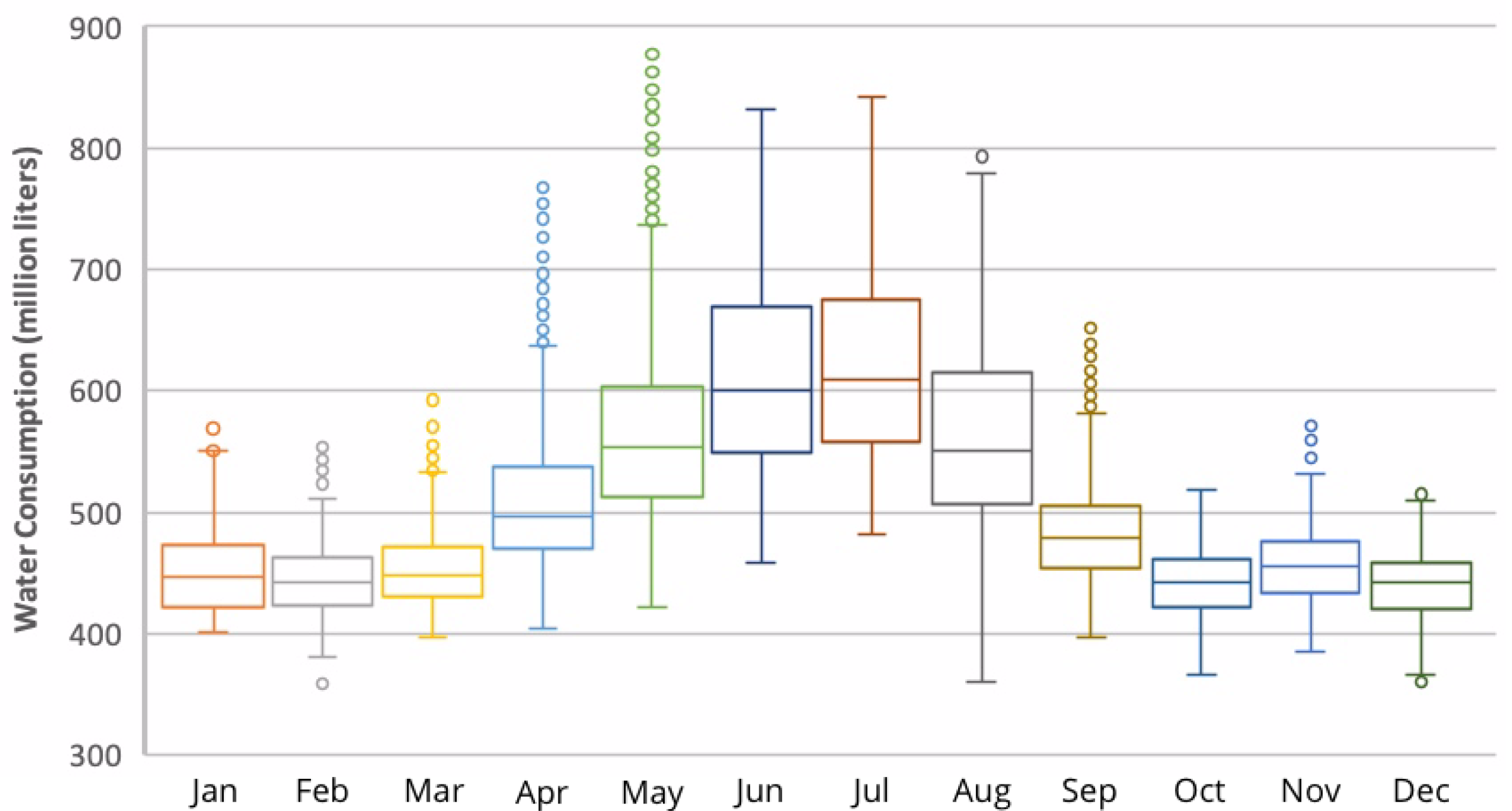
The data used in this paper was collected for a water distribution service area (Figure 1) in central Indiana from 1997 to 2017. Figure 2 shows a box-plot of the water consumption throughout the study period. The bottom line in each box in Figure 2 is the first quartile, the middle line is the median and the top line is the third quartile of the water consumption levels for the corresponding month of the year. The upper and lower whiskers are $1.5\times$ (third quartile - first quartile) above the third quartile and below the first quartile, respectively. This figure shows that water consumption is the highest during the summer months of May through September. A large number of deviations from the median are also observed during these months. For the remainder of the year (i.e., January through April and October through December), the consumption is largely constant with limited deviations from the median values.

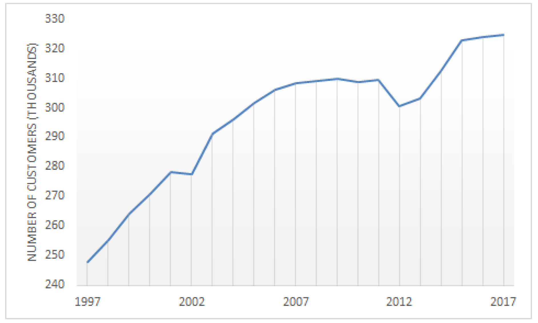
The customer count (Figure 3) for the service area is also collected. It is only available on a yearly basis with an average increase of 1.37% from one year to the next over the study period. The customer count reached 324,500 in 2017.

In addition to the operational data, three external data sets relevant to the study were collected. The first external data set connects observed water consumptions to the weather conditions. Weather data from seven weather stations within the service area were obtained from the National Oceanic and Atmospheric Administration’s (NOAA) National Climatic Data Center (NCDC) [24] database. The seven weather stations are USC00121303, USC00121326, USC00124260, USC00124272, USC00124286, USW00053842 and USW00093819. They were all active during the target time period from 1997–2017 and their geographical locations are overlaid on the service area map in Figure 1. For some stations, weather data were missing for some days (i.e., not recorded for the day). When available, the daily values of minimum temperature, maximum temperature, rainfall, snow and snow depth from each of the stations for each day were extracted. The mean values for each type of weather data were then calculated based on these available values.

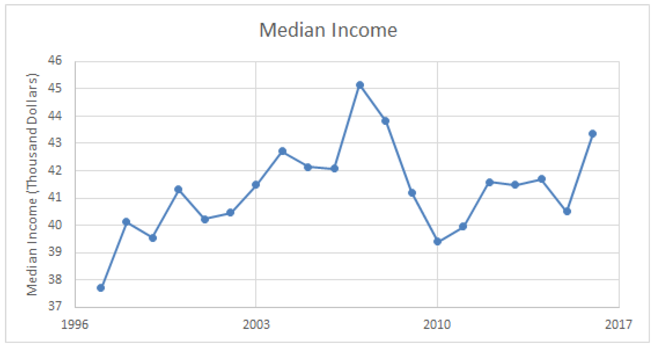
The second external data consisted of the median household income of the service region. It was obtained from the US Census Bureau [25] for the county (i.e., Marion County). As shown in Figure 4, the highest median income was in 2007 and the lowest was in 1997. The median income for 2017 is unavailable at the time of this publication.

The third external dataset is the calendar with holidays and major observances [26]. This data set includes all the major public holidays, bank holidays and observances (e.g., Halloween) which may not be holidays but are widely celebrated across the US.

4. Predicting Water Demand

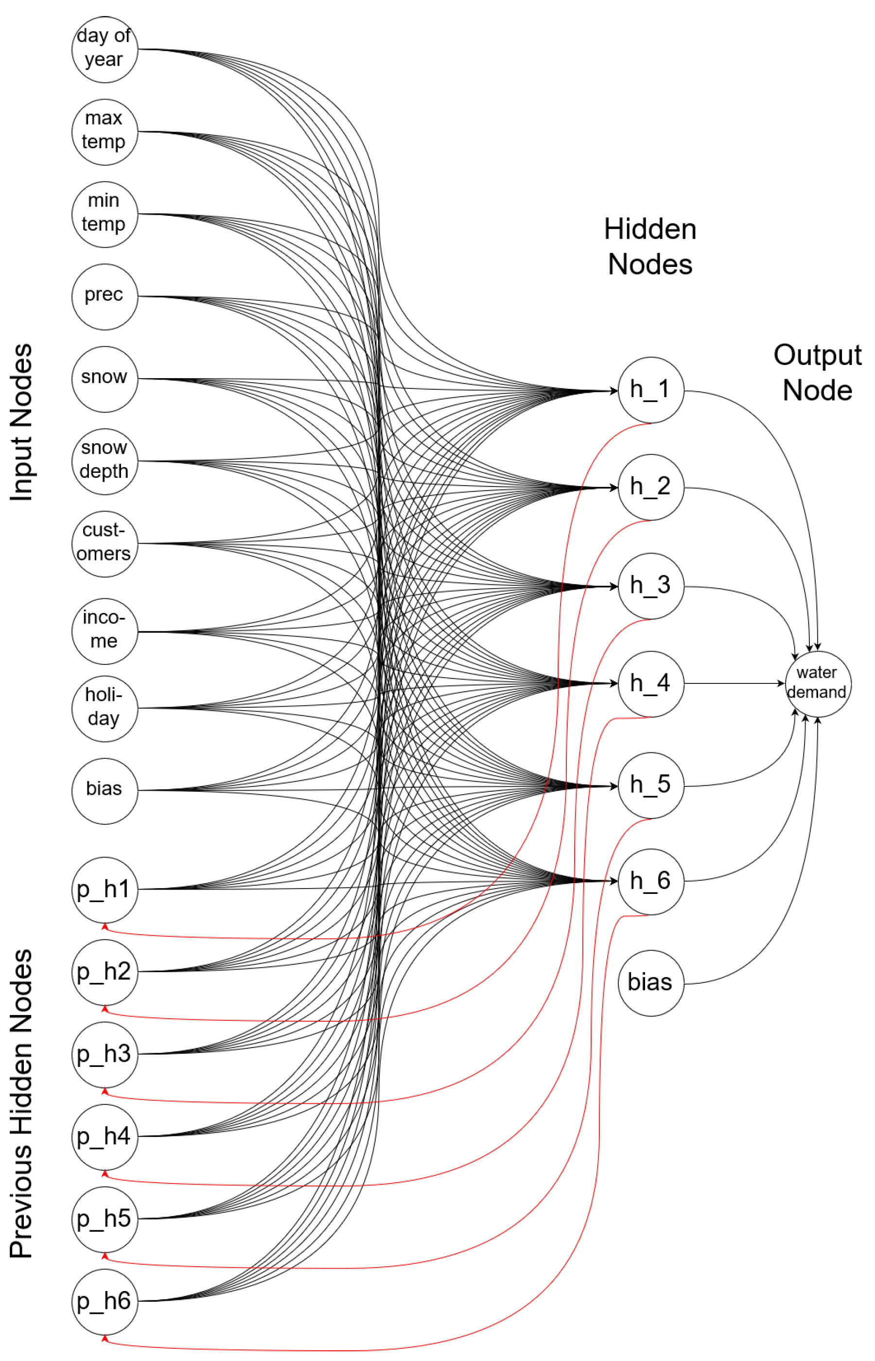
A recurrent neural network water demand model for the target service area was developped in [1]. This model (Figure 5) consists of ten input nodes, namely, day of the year, maximum temperature, minimum temperature, rainfall, snow, snow depth, number of customers, median income, holiday and a positive bias set to 1. The hidden layer consists of eight nodes and a positive bias node. The hidden layer values from the current day are used in the prediction of the next day’s water consumption. This hidden layer recurrence is based on the approach proposed in [27].

The output of the nodes in the hidden layer is calculated as follows,

$$H_j=tanh\left(h_j\right)where{h}_j=\sum _{i=1}^n{w}_{ij}^h·x_i$$

(1)

and $x_i$ represents the input node i, $w_{ij}^h$ represents the value of the weight from the input layer node $x_i$ to the hidden layer node $H_j$ and n is the total number of input nodes.

Similarly, the output ($\tilde{O}$) is calculated as follows,

$$\tilde{O}=tanh\left(\tilde{o}\right)where\tilde{o}=\sum _{j=1}^m{w}_j^o·H_j$$

(2)

and $w_j^o$ represents the weight from the hidden layer node $H_j$ to the output node and m is the number of hidden nodes.

The resulting network is a three-layer network: input, hidden and output. During the training of the model, backpropagation [28] is used to propagate the error from the output layer to the input layer and to update the weights in the network. The weights from the hidden layer to the output layer are updated by using the following error correction term

$$\Delta w_j^o=\alpha ·(\widehat{O}-\tilde{O})·\frac{\partial \tilde{O}}{\partial \tilde{o}}·H_j$$

(3)

where $\alpha$ is the learning rate, $\widehat{O}$ is the target value and $\frac{\partial \tilde{O}}{\partial \tilde{o}}$ is the partial derivative of the output $\tilde{O}$ with respect to $\tilde{o}$. Similarly, the weights of the network from the input layer to the hidden layer are updated as follows:

$$\Delta w_{ij}^h=\alpha ·(\widehat{O}-\tilde{O})·w_j^o·\frac{\partial \tilde{O}}{\partial \tilde{o}}·\frac{\partial H_j}{\partial h_j}·x_i$$

(4)

The accuracy of the models is measured by comparing the predicted values to the actual observations according to the following equation:

$$e=\frac{|\widehat{o}-\tilde{o}|}{\widehat{o}}\times 100$$

(5)

The average error ($\overline{e}$) for the model is then obtained by calculating the average of the errors (e) for all the predicted values in the testing period as follows:

$$\overline{e}=\frac{1}{p}\sum _{k=1}^p{e}_k$$

(6)

where p is the number of data points and $e_k$ is the error for the corresponding data point k.

The predictive importance of each input feature is evaluated by using the following metric:

$$I{W}_i=\frac{{\sum }_{j=1}^m\left|w_{ij}^h\right|}{{\sum }_{i=1}^n{\sum }_{j=1}^m\left|w_{ij}^h\right|}\times 100$$

(7)

where the numerator corresponds to the weights from the input layer to the hidden layer for a specific input feature i.

For each month, a different recurrent neural network is developed for a total of 12 networks. The output of the hidden nodes for the 1st of January is used as an input in the prediction of the water consumption for the 2nd of January, and so forth. At the end of the month, on the 31st of January, the hidden layer output is stored and used as an input for next year’s 1st of January. The initial values of the previous hidden layer nodes for each network are set to 0 during the training of the model. During testing, the initial values of the previous hidden layer nodes are set to the output of these nodes from the last training iteration of the model.

Offline training is performed using the data spanning 1997 to 2010. This step is followed by an online training and testing step by using the data from 2011 to 2017. The online training process updates the weights once for each data point (i.e., one epoch for each data point). This approach assumes that the actual water consumption is available at the end of the day. This value is used to update the weights by using Equations (3) and (4) and to predict the next day’s water consumption. 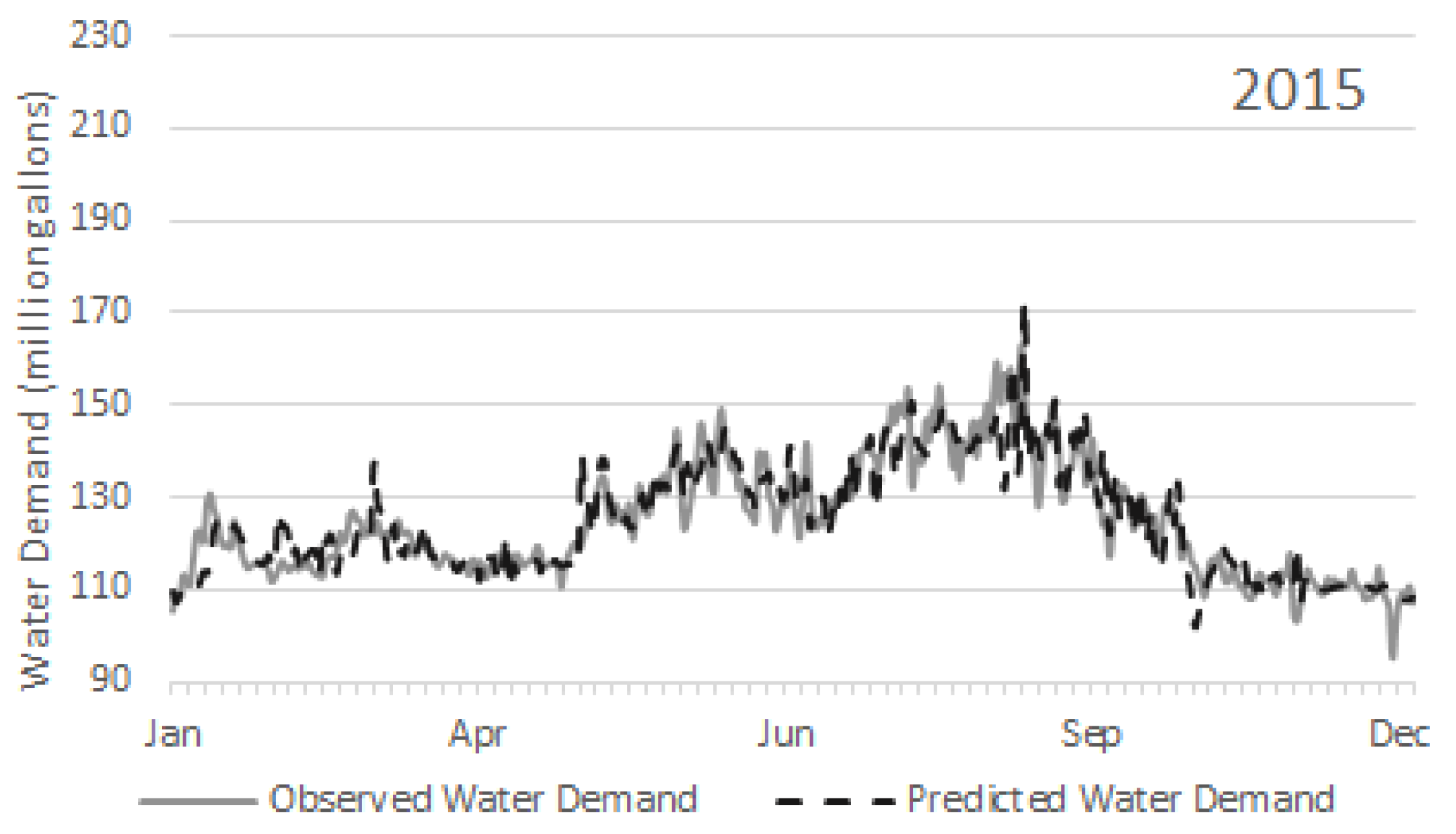The model developed using this training approach and the features described above is labeled original model [29]. The predicted water demand produced by the original model compared to the observed water demand for 2015 is shown in Figure 6. The online training and testing for the period 2011–2016 produced an average error ($\overline{e}$) of less than 4% as shown in

Table 1. Yearly average error ($\overline{e}$) for the original and reduced-feature models during the online testing period of 2011–2017 (in percent).

Year	Original Model	Reduced Model
2011	3.59	3.14
2012	4.61	3.82
2013	3.87	3.04
2014	3.81	3.20
2015	3.30	2.63
2016	3.36	1.67
2017	–	2.39
Average	3.76	2.84

. In general, the error kept decreasing as the model was trained with data from 2012 to 2016. In the case of the original model, 2017 was not included in the testing period because the income, one of the features of the model, was not available at the time of this publication. Few years in Table 1 show an increase in average error with respect to the previous year. Most of these increases, as will be discussed in Section 5, are due to the number of outlier days in that year.

Based on the results in Table 1 and by evaluating the $IW$ values, feature reduction was performed on the original recurrent neural network model, and the input features with low $IW$ were omitted. A reduced configuration of the model consisting of four input nodes was created. The input nodes are: (1) day of the year as a bitonic function increasing from 1 to 183 during the first half and decreasing from 183 to 1 during the second half of the year; (2) maximum temperature; (3) precipitation as the sum of rainfall and snow and (4) an input bias. The number of hidden nodes in the reduced model was set to 8. The recurrence pattern was maintained and 12 networks, one for each month, were created. The day of the year was normalized with respect to the difference ($D=182$) between the maximum and minimum values across the study period by using the following equation:

$$\tilde{x}=tanh\frac{x-\frac{D}{2}}{\frac{D}{4}}$$

(8)

where $\tilde{x}$ is the normalized value for each data point x. The normalization of the temperature and precipitation is with respect to $D=5\sigma$ where $\sigma$ is the standard deviation of the temperature and precipitation, respectively.

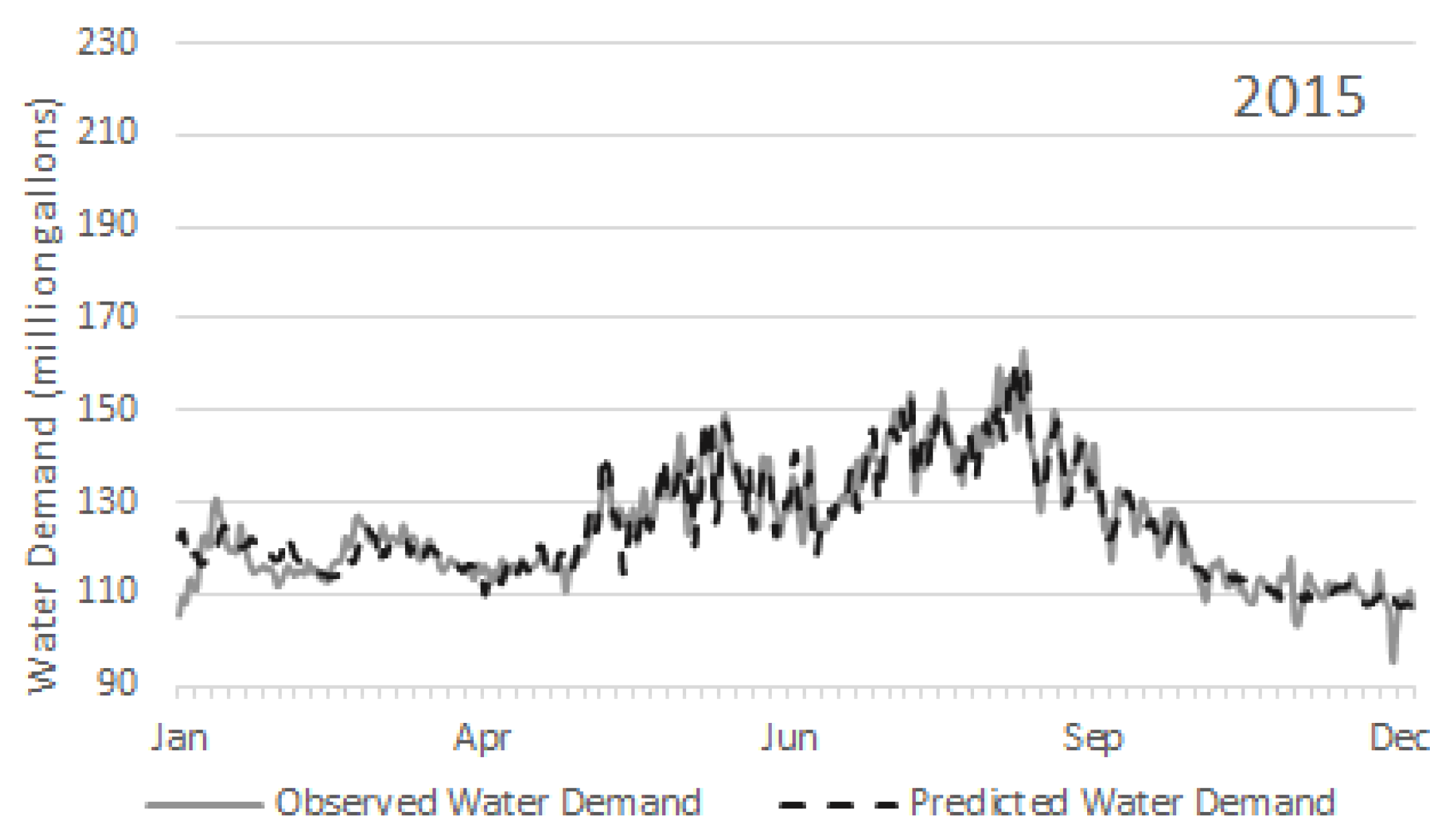
The predicted output using the reduced model compared to the actual water consumption levels for 2015 is shown in Figure 7. Table 1 also shows the average prediction errors for the reduced model over the period 2011 to 2017. The average error for the original model in 2011 is 3.59% whereas it is 3.14% for the reduced model. As in the case of the original model, the average error generally reduces throughout the online training for the reduced model. However, this trend is not consistent for the years 2012 and 2017. In the case of 2012, the deviation from the trend is due to under-consumption during the June–September period as a result of mandatory restrictions. For 2017, the deviation is due to over-consumption during the months of August and September and to under-consumption during the months of November and December.

The values of $IW$ (Equation (7)) obtained for the reduced model are shown in

Table 2. Importance of weight ($IW$) of each input feature in the reduced model, for each month over the period from 2011 to 2015. In addition to the bias node, the features are DoYr: day of the year, MxTp: maximum temperature, Prcp: precipitation and PHL: previous hidden layer.

	DoYr	MxTp	Prcp	Bias	PHL
January	29.53	2.42	0.50	26.41	41.15
February	16.39	2.57	6.64	14.08	60.32
March	9.82	1.68	2.66	9.92	75.92
April	10.28	6.65	6.62	20.60	55.85
May	10.97	30.79	3.67	37.33	17.24
June	15.82	27.21	1.97	40.79	14.21
July	15.86	39.01	2.46	26.77	15.90
August	4.83	24.73	3.02	28.33	39.09
September	6.93	23.86	5.72	31.31	32.18
October	16.06	14.26	4.79	20.60	44.29
November	13.68	2.08	5.80	14.13	64.31
December	12.65	3.32	1.70	15.72	66.61

. These $IW$s show a strong correlation between the water demand and two input features: day of the year and the previous day’s hidden layer values throughout the year. The dependence on the previous day’s hidden layer values captures the autoregressive component of water demand [30]. It is also the main reason for the improved performance of the proposed recurrent neural network model compared to the feed forward neural network model [1].

The dependence of the water demand prediction on the maximum temperature is low for the low demand months of January–April and November–December whereas, the dependence on maximum temperature is high for the high demand months of May–September. This confirms the correlation between maximum temperature and high water demand during the summer months. Moreover, the model’s dependence on precipitation is low and indicative of the lesser importance of this feature in the service area.

In addition to the original and the reduced features recurrent networks, four variant configurations were investigated. In the first configuration, precipitation was encoded as a binary (i.e., 0 or 1) input feature instead of a scaled input. In the second configuration, the hidden layer node values were propagated throughout the year instead of on a monthly basis. That is, the hidden layer values for 31 January 1997, were used as an input to the 1 February 1997, instead of as an input for the 1 January 1998. Both of these variant configurations failed to improve the accuracy of the prediction. In the third and fourth variant configurations, input recurrence and output recurrence were used in the reduced feature set model instead of the proposed hidden layer recurrence, respectively. Again, both of these configurations under-performed compared to the original recurrent network model and the reduced feature model with hidden layer recurrence. The input layer recurrent network had an average error of 4.16% and the output layer recurrent network produced an average error of 3.65%.

5. Differential Learning Prediction Models

Despite the low average error obtained over the 7 year testing period (Table 1), there are days with high prediction errors. In some cases, prediction errors can reach up to 66% for the reduced feature model. This is particularly true for the months of May to September. These months correspond to high water consumption months as exemplified by Figure 6.

In the remainder of this section, days with prediction errors $\ge \pm 10\%$ are defined as outliers. Using this definition, a large number of the outliers occur during the summer months and are associated with days that register maximum temperatures greater than 29 ${}^{\circ }$C. A recurrent neural network configuration with an additional input indicating maximum temperature greater than 29 ${}^{\circ }$C was tested. Unfortunately, this configuration produced worse results because there were a significant number of days with temperature greater than 29 ${}^{\circ }$C but with normal water consumption levels.

In addition to days with high temperatures, operational practices may also induce outliers in water demand. For instance, utility companies can have voluntary or mandatory watering restrictions days. These restrictions limit the levels of water consumption. For the data set used in this study, mandatory restrictions were enforced only once during the study period for 55 days from 07/13/2012 to 09/05/2012. Voluntary restrictions were advised twice. The first voluntary restriction was for 6 days from 06/14/2007 to 06/19/2007. The second voluntary restriction was for 7 days from 07/06/2012 to 07/12/2012. These restrictions led to higher average prediction errors in 2012 (Table 1) for both the original and the reduced feature models. A configuration of the model that takes into account watering restrictions as a binary input feature was also investigated. However, this configuration did not improve the prediction accuracy.

5.1. Positive and Negative Outlier Networks

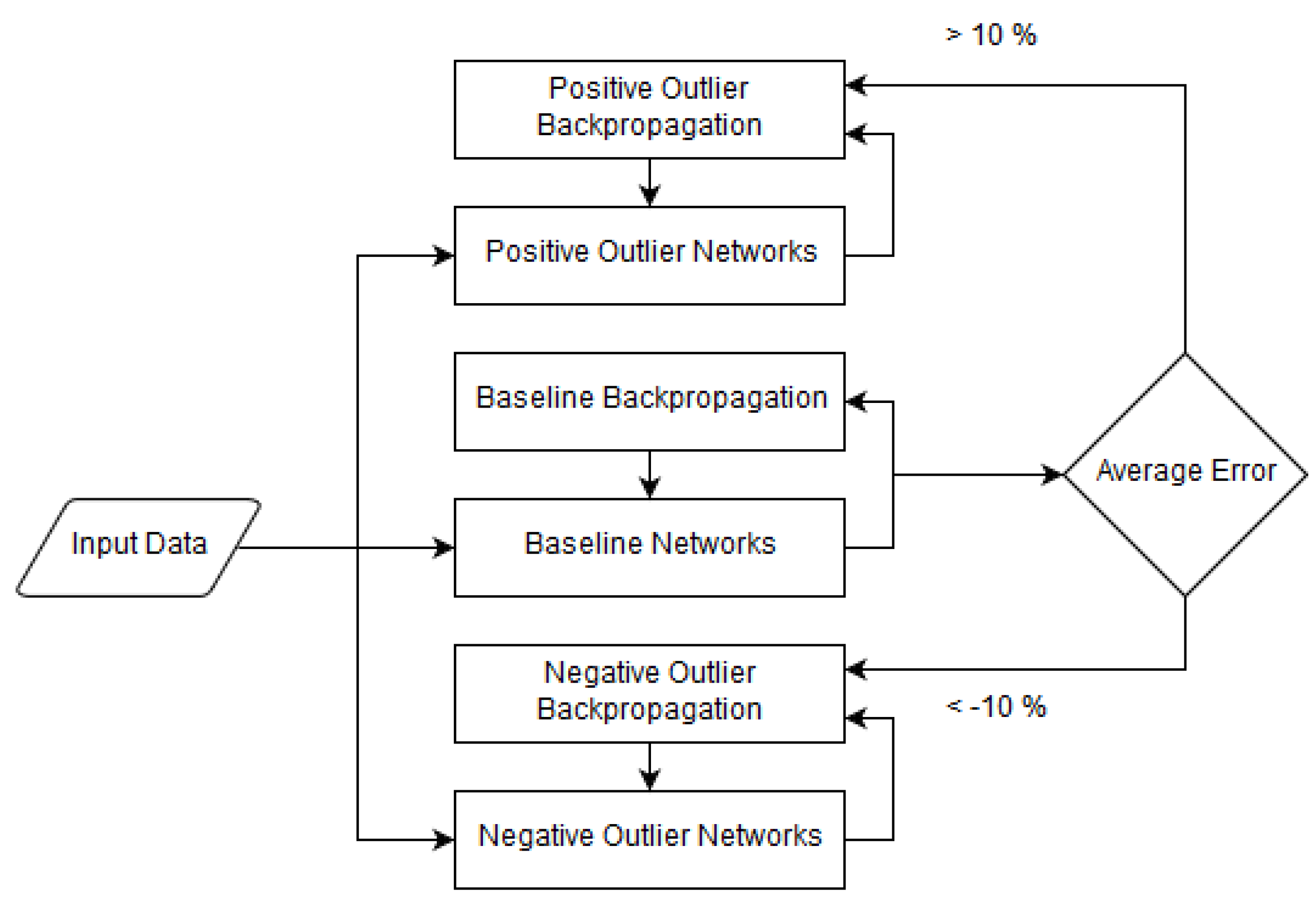
To estimate the water demand for outlier days as a result of restrictions or under/over-consumption a differential learning model is proposed. The new model includes the reduced feature model as the baseline, along with parallel network(s) for outlier range estimation. The general configuration of the proposed model is shown in Figure 8.

The first differential learning model investigated consisted of the 12 reduced features monthly recurrent networks (baseline network) and one single outlier network. The additional outlier network is also a recurrent network and was trained by using only the data points with an error $\ge \pm 10\%$. The baseline network was trained by using the data points that produced an error $\le \pm 10\%$. For each predicted data point in the differential network, the error is calculated as the minimum error of either the baseline network or the outlier network compared to the actual consumption level. With this configuration, the error improved for some of the over-consumption days. However, the error increased for under-consumption days. The average error for this model was 2.59%.

The above result indicates that over-consumption should be treated differently from under-consumption. Therefore, a new configuration was developed. This configuration consisted of the same baseline network and two outlier networks, one for positive outliers (over-consumption) and one for negative outliers (under-consumption). Moreover, for this new configuration, the baseline network was trained by using all the data points, the positive outlier network was trained by using data points with error $\ge 10\%$ and the negative outlier network was trained by using data points with error $\le -10\%$. This training approach is referred to as Training Method A in the remainder of the paper. The resulting model produced an average error of 2.36% for 2011–2017 as show in

Table 3. Average error for the differential prediction configuration networks with one positive and one negative outlier networks over the period 2011–2017. Outlier threshold is set to 10%.

Training Method	Average Error
Method A: Baseline network trained on all data points	2.36%
Method B: Baseline network not trained on outliers	2.87%
Method C: Outlier networks trained after 50,000 epochs	2.31%

. This error is lower than that of both the original and the reduced feature recurrent network models shown in the last row of Table 1.

Other training strategies were also tested. In the first variant, the baseline network was trained by using only the data points that produced an error less than $\pm 10\%$ (Training Method B). That is, the positive and negative outlier data points were not used in the training of the baseline network. The training of the positive and negative outlier networks was maintained as in Method A. The resulting average error for this training approach over the testing period from 2011–2017 was 2.87% (Table 3). This error is higher than the previously obtained average error where the baseline network was trained with all the data points.

A third training approach (Training Method C) was also investigated in order to help avoid overfitting in the outlier networks. In this method, the training of both the positive and the negative outlier networks is delayed 50,000 epochs after the start of the training of the baseline network. Training Method C has an improved average error compared to Training Method A (Table 3). Overfitting can occur in the outlier networks because of the limited number of outlier data points [23].

Table 4. Total number of positive and negative outliers occurring each month over the period 2011–2017.

	Positive Outliers	Negative Outliers	Total
January	23	63	86
February	19	68	87
March	10	46	56
April	4	50	54
May	7	85	92
June	26	73	99
July	40	64	104
August	30	45	75
September	15	50	65
October	5	82	87
November	5	63	68
December	15	68	83
Total	199	757	956

shows the number of these outliers for each month over the period 2011–2017. Most of the outliers are negative (i.e., under-consumption). Moreover, the number of positive outliers (i.e., over-consumption) during the months of July-September are much higher than the rest of the year.

A review of the number of outliers over the time period of this study shows that on average, the period from 2011–2015 had more outliers than the period 2016–2017. The proposed machine learning model is sensitive to variations in the distribution of the outliers. Understanding this variation is therefore important for the development of an accurate predictive model. For example, due to the distribution of the outliers in the water demand data set, the differential learning model improved accuracy prediction for the period 2011–2015 more than for the period 2016–2017.

5.2. Analysis

The previous section investigated various configurations of the proposed differential learning network. The results show that two outlier networks [one positive and one negative] produce better results than a single outlier network. The results also indicate that the best performance is obtained when the baseline network is trained using all the data points and the training of the outlier networks is delayed with respect to the baseline network (Training Method C).

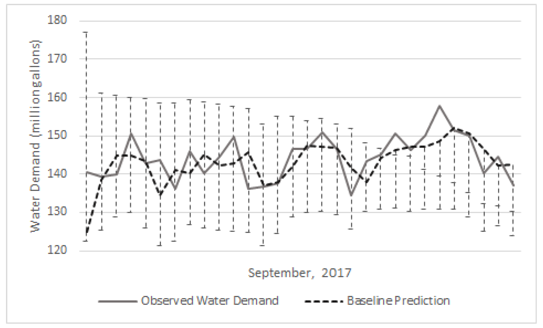
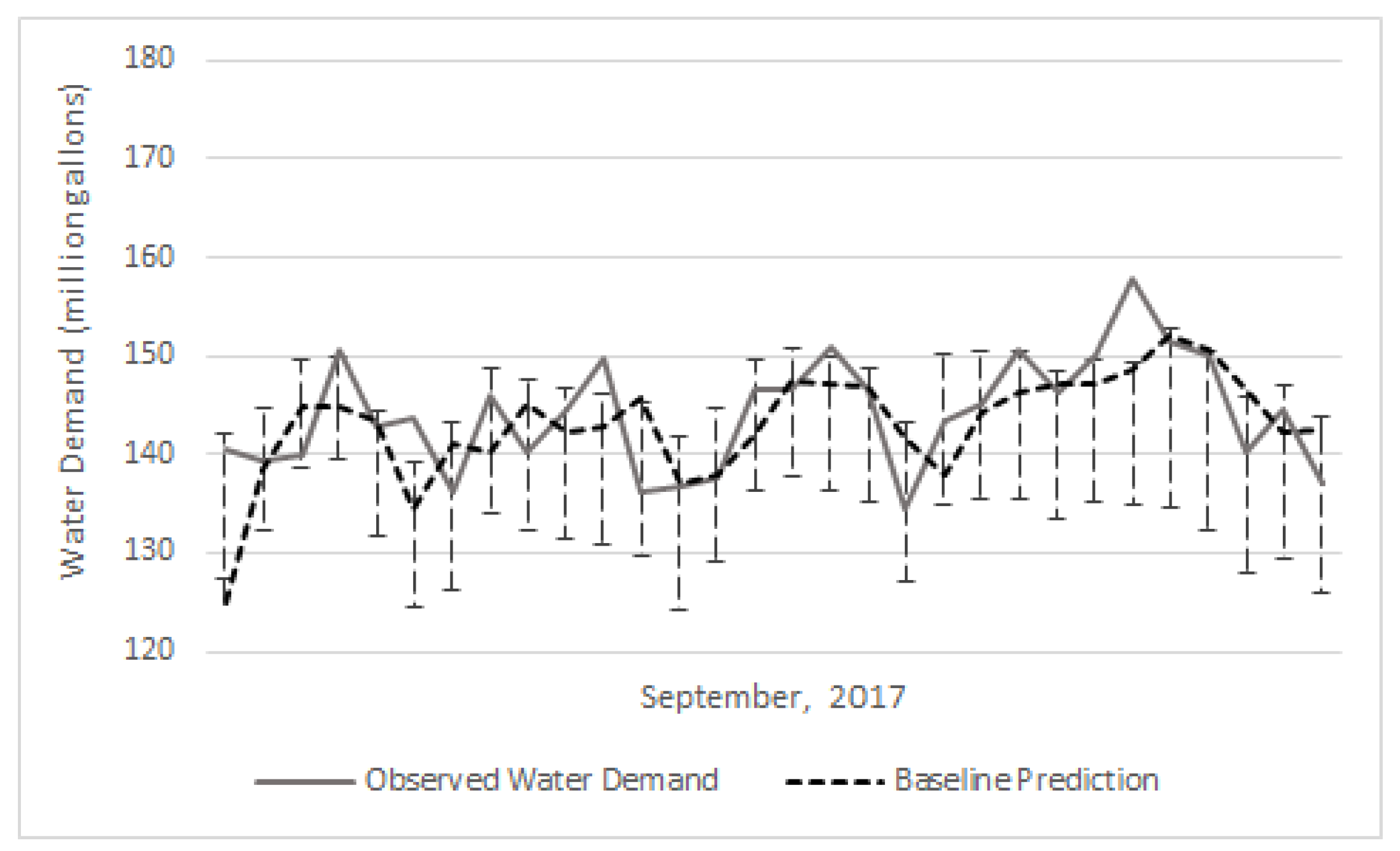
The purpose of the outlier networks in the proposed differential learning model is to generate low and high estimates of the daily water demand. Because the outlier networks are trained with outlier data points defined with respect to a threshold (i.e., $10\%$), the resulting model and estimates are sensitive to this threshold. Figure 9 shows the output of the baseline network and that of the outlier networks for the month of September 2017 by using training Method C and an outlier threshold of 10%. The threshold was then reduced to 5% (Figure 10) and the corresponding differential learning network model produced and average error of 1.90%. This approach of refining the threshold was also succesfully used for one class of outliers in [23].

With a larger threshold, the outlier estimates tend to exceed the observed demand by a large margin. Reducing the threshold from 10% (e.g., Figure 9) to 5% (e.g., Figure 10) shows better estimates. The choice of the threshold is application-dependent and would have to be calibrated for each service area. Moreover, choosing a very low threshold may eliminate the benefits of the outlier networks as they will be trained using most of the data points used to train the baseline network and therefore, would generate predictions similar to those of the baseline network.

To evaluate whether the features that are important for the baseline network are also important for the outlier networks, the importance ($IW$) of the input features in the outlier networks were calculated as shown in

Table 5. Importance of weights ($IW$) of each input feature in the positive and negative outlier networks for the period of 2011–2015.

Outlier Network	DoYr	MxTp	Prcp	Bias	PHL
Positive	4.79	20.03	3.18	19.68	52.31
Negative	2.61	36.69	2.03	37.39	21.28

. Compared to Table 2, the $IW$ of the day of the year is significantly lower for both the positive and negative outlier networks. In the case of the positive outlier network, this $IW$ is close to that of the summer months of August and September in the baseline network. This result can be explained by the fact that the majority of the positive outliers occur in the months of July–September (Table 4). These months also have the highest water consumption levels.

The dependence on the maximum temperature is high for both outlier networks. The positive outlier network has an $IW$ for maximum temperature equivalent to that of the summer months May–September in the baseline model. This was anticipated. However, the $IW$ (≈37%) of the negative outlier network for this input feature was not expected and aligns with the fact that some of the days with high temperatures result in under-consumption compared to the baseline. A similar observation was made in [9] where fluctuations during spring and summer were found to be more pronounced than during the autumn and winter.

The $IW$ of precipitation is low for both outlier networks and has a similar value to that of the baseline network. However, eliminating this input feature from either the baseline or outlier networks yields a lower accuracy.

6. Conclusions

This paper proposes a differential learning model that can estimate lower and upper bounds for water demands. The model consists of a baseline network in parallel with a positive outlier network for over-consumption and a negative outlier network for under-consumption. The results show that one outlier network is not sufficient to estimate both over and under consumption. Furthermore, the results show that a delayed training of the outlier network with respect to the baseline network can help overcome overfitting since the number of outliers is usually limited. The results also show that better average prediction errors are obtained when the baseline network is trained with all data points including the outliers.

The baseline network consists of 12 recurrent networks one for each month of the year. Hidden layer recurrence is used for each network. The threshold for the outliers was initially set to 10%. This value was later reduced to 5%. Reducing the threshold improves the accuracy of the network. However, reducing the threshold any further renders the outlier networks unnecessary since they start producing the same water demand prediction as the baseline. The choice of the appropriate threshold level is application dependent.

The proposed model was trained and tested on an actual data set from a water utility company in central Indiana. The network was trained by using daily water demands from 1997 to 2010. Online training of the model was then continued by using daily water demands from 2011 to 2017. The baseline model was tested over this latter period and had an average error of 2.84%. The differential learning network model had an average error of 2.31% and 1.90% with threshold values of 10% and 5%, respectively.

Future work will investigate the use of the proposed model for other applications. Furthermore, we would like to develop a systematic approach that can help determine a suitable value for the outlier threshold.