Side-Channel Vulnerabilities of Unified Point Addition on Binary Huff Curve and Its Countermeasure

Abstract

Unified point addition for computing elliptic curve point addition and doubling is considered to be resistant to simple power analysis. Recently, new side-channel attacks, such as recovery of secret exponent by triangular trace analysis and horizontal collision correlation analysis, have been successfully applied to elliptic curve methods to investigate their resistance to side-channel attacks. These attacks turn out to be very powerful since they only require leakage of a single power consumption trace. In this paper, using these side-channel attack analyses, we introduce two vulnerabilities of unified point addition on the binary Huff curve. Also, we propose a new unified point addition method for the binary Huff curve. Furthermore, to secure against these vulnerabilities, we apply an equivalence class to the side-channel atomic algorithm using the proposed unified point addition method.

1. Introduction

Side-channel attacks (SCAs) are major threats to the security of cryptographic embedded devices. Power analysis, the most actively researched SCA technique, can be used to find secret information by using the power consumption data extracted during the cryptographic operations of embedded devices. Power analysis attacks on elliptic curve cryptosystems (ECCs) are classified into two types: simple power analysis (SPA) and differential power analysis (DPA) [1]. SPA exposes secret information by observing the power consumption of a single execution of a cryptographic algorithm. For example, a secret key can be easily extracted from the binary scalar multiplication algorithm by differentiating the point addition signal from the point doubling signal. On the other hand, DPA reveals secret information by statistically analyzing many executions of the same algorithm with different inputs without the physical decapsulation of the target device, even if it is impossible to apply SPA. DPA utilizes a correlation between power consumption and specific key-dependent bits that appear at the cryptographic computations. Among the representative countermeasures against DPA are randomization techniques, e.g., scalar/message blinding methods and randomized projective coordinates, which make it impossible to guess the specified values [2]. The countermeasures against SPA can be divided into two main categories. The first strategy is to perform point addition and point doubling, regardless of the secret bit value, such as the double-and-add-always method and Montgomery ladder algorithm [2,3]. The second approach is to make basic operations indistinguishable, such as side-channel atomicity and unified point addition [4,5].

Recently, two new SCAs using only one power consumption trace—recovery of secret exponent by triangular trace analysis (ROSETTA) and horizontal collision correlation analysis (HCCA)—have been proposed to analyze various countermeasures against DPA and SPA [6,7]. While ROSETTA can find secret information by distinguishing whether the operands of a field multiplication are the same or different, HCCA can find it by distinguishing whether the two field multiplications have at least one operand in common. These two attacks do not require any prior knowledge of the input operands of the field multiplications.

Unified point addition is useful for resisting ECCs to SPA. This technique, by which point addition and point doubling use the same sequence of field operations, was first introduced by Brier and Joye in affine and projective coordinates [5]. After that, various unified point addition formulae were proposed for their application to many kinds of elliptic curves, such as Edwards curves, binary Huff curves, and so on. Recently, unified point addition for the binary Huff curve was proposed by Debigne and Joye at the CT-RSA 2011 conference [8]. However, at the CHES 2013 conference, S. Ghosh et al. showed that unified point addition was insecure against SPA. They further proposed a modified unified point addition formula for the binary Huff curve which would provide resistance to SPA [9].

In this paper, we demonstrate two vulnerabilities of unified point addition on the binary Huff curve using ROSETTA and HCCA. Unified point addition operates with an identical sequence of field operations, regardless of the input points. However, some field multiplications of the unified point addition computation can be affected by investigating whether the two input points are equal or not. If two input points of the unified point addition operation are equal, field multiplications are computed with the same operands (i.e., squaring). Also, there are some field multiplication pairs with common operands. Hence, unified point addition can be exposed to the risk of these vulnerabilities using ROSETTA and HCCA. In order to show that unified point addition actually has these weaknesses, we implemented unified point addition on a binary Huff curve on an ARM cortex-m4 processor that performs field multiplications depending on the secret bit value, repeatedly. Then, we analyzed a power consumption trace collected from the implementation by using our attack methods. As a result of the actual experiments, we were able to find secret bit values more than 94% of the time, which proves that this unified point addition operation is indeed vulnerable to our attacks, and the single trace attack is a practical threat.

To provide security against our attack methods, we propose a new countermeasure using an equivalence class for unified point addition. By using the equivalence class, even though two input points of the unified point addition operation are in the same class, the two points can be different projective coordinate values. In addition, to provide perfect security against our attack methods, we reconfigured the operations of the unified point addition formula. The proposed unified point addition method for the binary Huff curve using the equivalence class is just about 2∼4.4% slower than the existing unified point addition method from [8,9]. In addition, the proposed method is about 8.5∼17.5% faster than an existing countermeasure that provides same security, i.e., unified point addition using blinding operands of a field multiplication [10]. We applied the aforementioned attacks to the unified point addition formulae of other elliptic curves and confirmed that most unified point addition formulae have these vulnerabilities.

This paper is organized as follows. Section 2 introduces basic knowledge of binary Huff curves and a description of ROSETTA and HCCA. In Section 3 and Section 4, we explain the vulnerabilities of the unified point addition formulae and describe the experimental results of applying these methods. Section 5 proposes our method to make unified point addition secure against our attacks. In Section 6, we compare the proposed method with previous methods. Finally, Section 7 addresses our conclusions. In addition, we explain the vulnerabilities of several unified addition formulae and their countermeasures in the Appendix A.

2. Preliminaries

2.1. Binary Huff Curve and Unified Point Addition

At CT-RSA in 2011, a Huff curve for the binary field was proposed by Devigne and Joye. Instead of providing general point addition, this construction provides a unified point addition operation to resist side-channel attacks. However, at CHES in 2013, Ghosh et al. demonstrated that the unified point addition method from CT-RSA 2011 was insecure against SPA. Even though both point addition and point doubling are computed with the same formula and executed by the same sequence of finite field operations, they demand different amounts of power consumption. Specifically, point doubling with unified point addition produces a zero value in some intermediate operations. However, point addition does not. Such zero values in point doubling are used in some field multiplications in unified point addition. Apparently, the outputs are also zero. The power consumption of these multiplications with zero and nonzero inputs are significantly different. Therefore, it is possible to distinguish between point doubling and point addition. Hence, they proposed a new unified point addition formula which is secure against SPA. Here, we provide a brief description.

Definition 1

([11]). A generalized binary Huff curve is the set of projective points $(X:Y:Z)\in {\mathbb{P}}^2\left({\mathbb{F}}_{2^m}\right)$ satisfying the equation

$$E/F_{2^m}:aX(Y^2+fYZ+Z^2)=bY(X^2+fXZ+Z^2),$$

(1)

where $a,b,f\in {\left(F\right)}_{2^m}^{*}$ and $a\ne b$.

There are three points at infinity that satisfy the curve equation, namely, $(a:b:0)$, $(1:0:0)$, and $(0:1:0)$. Let $P_1=(X_1:Y_1:Z_1)$ and $P_2=(X_2:Y_2:Z_2)$; then, we get $P_1+P_2=(X_3:Y_3:Z_3)$ with unified point addition [8]:

$$\left\{\begin{array}{c}{X}_3=(Z_1{Z}_2+Y_1{Y}_2)((X_1{Z}_2+X_2{Z}_1)(Z_1^2{Z}_2^2+X_1{X}_2{Y}_1{Y}_2)+\hfill \\ \alpha X_1{X}_2{Z}_1{Z}_2(Z_1{Z}_2+Y_1{Y}_2))\hfill \\ Y_3=(Z_1{Z}_2+X_1{X}_2)((Y_1{Z}_2+Y_2{Z}_1)(Z_1^2{Z}_2^2+X_1{X}_2{Y}_1{Y}_2)+\hfill \\ \beta Y_1{Y}_2{Z}_1{Z}_2(Z_1{Z}_2+X_1{X}_2))\hfill \\ Z_3=(Z_1{Z}_2+X_1{X}_2)(Z_1{Z}_2+Y_1{Y}_2)(Z_1^2{Z}_2^2+X_1{X}_2{Y}_1{Y}_2),\hfill \end{array}\right.$$

(2)

where $\alpha =(a+b)/b$ and $\beta =(a+b)/a$. The unified point addition formula in Equation (2) can be evaluated as described in [9]:

$m_1=X_1{X}_2,$    $m_2=Y_1{Y}_2,$    $m_3=Z_1{Z}_2,$

$m_4=(X_1+Z_1)(X_2+Z_2),$    $m_5=(Y_1+Z_1)(Y_2+Z_2),$

$m_6=m_1{m}_3,$    $m_7=m_2{m}_3,$    $m_8=m_1{m}_2+m_3^2,$

$m_9=m_6{(m_2+m_3)}^2,$$m_{10}=m_7{(m_1+m_3)}^2,$    $m_{11}=m_8(m_2+m_3),$

$Z_3=m_{11}(m_1+m_3),$    $X_3=m_4{m}_{11}+\alpha m_9+Z_3,$

$Y_3=m_5{m}_8(m_1+m_3)+\beta m_{10}+Z_3.$

The above operation needs 17 field multiplications, which is exactly the same as in the original one. Since point doubling does not have a zero value in any intermediate operation, it is secure against SPA. Recently, however, SCAs such as SPA using only one power consumption trace have been proposed [6,7]. Therefore, security analysis of the unified point addition formula should be considered not only for SPA but also for other analyses. Using these analyses, we present the vulnerabilities of the unified point addition method from [9] and report our experimental results in Section 3 and Section 4, respectively.

2.2. ROSETTA and HCCA

Recovery of secret exponent by triangular trace analysis (ROSETTA) [7] and horizontal collision correlation attack (HCCA) [6] are based on the observations of the power consumption of the cryptosystems during the executions of field multiplications. They are powerful attacks on elliptic curve cryptosystems since they use only one power consumption trace for SPA. ROSETTA and HCCA can be used to reveal secret information by analyzing the correlation between the secret bit value and the power consumption of field multiplications without any prior knowledge of the inputs. Details of the analyses are as follows.

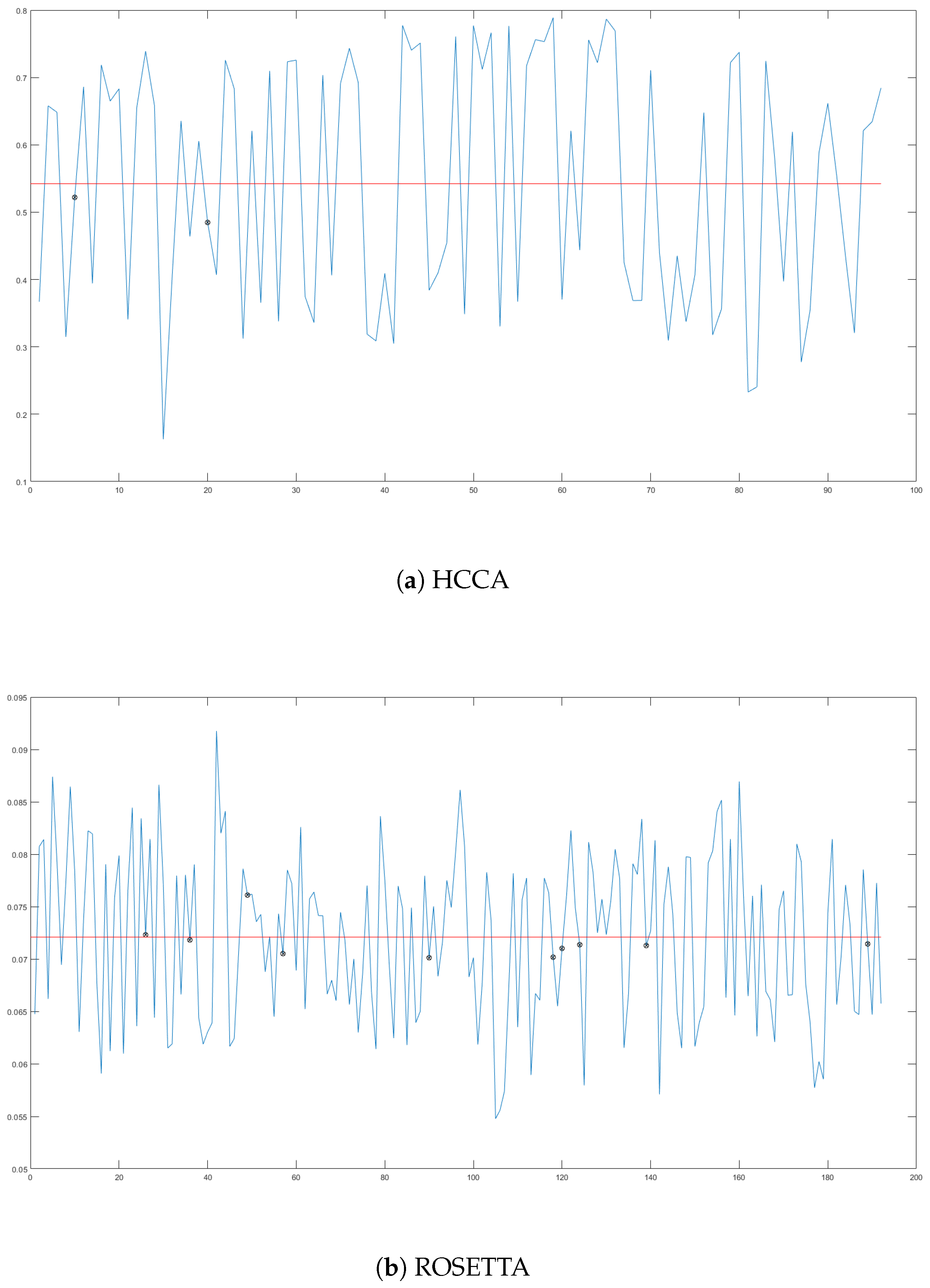
• ROSETTA. Clavier’s attack needs a single power consumption trace to recover secret information. For each field multiplication, ROSETTA detects whether the operation is $x·x$ (squaring) or $x·y$ (multiplication). Let $x={(x_{m-1},x_{m-2},...,x_0)}_{2^w}$ and $y={(y_{m-1},y_{m-2},...,y_0)}_{2^w}$. A w-bit multiplication $x_i·y_j$ can be identified from the specific pattern in side-channel power consumption. ROSETTA considers the observation $O_1$ and $O_2$ extracted from the multiplication $x_i·y_j$ for all $i\ne j$:
  $\left(O_1\right):$$x·y$ s.t $x=y$ ⇒ Prob($x_i·y_j=x_j·y_i$) $=1$ for all $i\ne j$
  $\left(O_2\right):$$x·y$ s.t $x\ne y$ ⇒ Prob($x_i·y_j=x_j·y_i$) $\approx 0$ for all $i\ne j$
  From the observations $O_1$ and $O_2$, collisions between $x_i·y_j$ and $x_j·y_i$ for all $i\ne j$ can be used to identify squarings from multiplications. To identify these collisions of field multiplication trace, ROSETTA exploits a triangle trace analysis which uses a Euclidean distance distinguisher relying on a collision correlation technique.
• HCCA. Bauer et al. introduced this method to extract keys using the collision of field multiplications in a single power consumption trace. The core idea of this attack is that collision occurs during two field multiplication computations when the same operands are used, which can be detected by HCCA. When performed in a horizontal setting, the observations $O_1$ and $O_2$ are extracted from the two field multiplications.
  $\left(O_1\right):$$x_1·y_1$ and $x_2·y_2$ s.t $x_1=x_2$ and $y_1=y_2$ ⇒ Prob(${\left(x_1\right)}_i·{\left(y_1\right)}_j={\left(x_2\right)}_i·{\left(y_2\right)}_j$) $=1$ for all $i,j$
  $\left(O_2\right):$$x_1·y_1$ and $x_2·y_2$ s.t $x_1\ne x_2$ and $y_1\ne y_2$ ⇒ Prob(${\left(x_1\right)}_i·{\left(y_1\right)}_j\ne {\left(x_2\right)}_i·{\left(y_2\right)}_j$) ≈ 0 for all $i,j$
  The correlation between the two observations is then estimated by Pearson’s coefficient in order to determine whether the two operands of the field multiplications are the same or different.

The advantage of these analyses is that the inputs of field multiplication can remain unknown since the adversary does not need to compute intermediate values. Countermeasures against ROSETTA and HCCA include shuffling the operands and blinding the operands of a field multiplication [10]. For n-bit field multiplication, the blinding operand method requires $t^2+2t+1$ w-bit multiplications, where $t=\lceil n/w\rceil$. Unified point addition using blinding operands requires a great additional computational cost. Therefore, for efficiency, we propose a suitable and efficient countermeasure for the unified point addition operation, and we compare and analyze the proposed method with the existing unified point addition method using blinding operands on the binary Huff curve.

3. Vulnerabilities of Unified Point Addition

Many methods have been proposed to prevent SPA, such as unified point addition and the Montgomery ladder algorithm. Since unified point addition can compute point addition and point doubling with the same formula, it is secure against SPA. In addition, it can be applied to various algorithms easily. In this section, we define two types of vulnerabilities of unified point addition and find vulnerabilities of unified point addition of the binary Huff curve in [9].

3.1. Vulnerabilities of Unified Point Addition

We describe the vulnerabilities of unified point addition considering ROSETTA and HCCA. Both are analyses using the correlation between the input data and operations. ROSETTA can determine whether the operands of a field multiplication are equal (squaring) or different (multiplication). HCCA can determine whether two field multiplications have the same or different operands. We defined the two types of vulnerabilities exposed by these analyses.

• Type 1. (Vulnerability by ROSETTA): The unified point addition operation can compute the point doubling and point addition with the same formula. However, depending on the input points of unified point addition, field multiplications can be performed as squaring or multiplication. For example, let $P_1=(X_1:Y_1:Z_1)$ and $P_2=(X_2:Y_2:Z_2)$ be the two input points of the unified point addition formula. Note that there exists the operation $X_1·X_2$ in unified point addition. If $P_1=P_2$, then this operation computes to $X_1·X_1$. If $P_1\ne P_2$, then this operation computes to $X_1·X_2$. Then, this operation becomes a vulnerability that is exploitable by ROSETTA.
• Type 2. (Vulnerability by HCCA): Considering two field multiplications, if they have at least one common operand, they can be distinguished by HCCA. In unified point addition, the two different multiplications can be identically computed according to the inputs. For example, the operations $X_1·Y_1$ and $X_2·Y_2$ exist in unified point addition. If $P_1=P_2$, then $X_1·Y_1$ will be computed twice. If $P_1\ne P_2$, then $X_1·Y_1$ and $X_2·Y_2$ will be computed. Then, these operations become a vulnerability that is exploitable by HCCA.

3.2. Vulnerabilities of Binary Huff Curve

In this section, we find Type 1 and Type 2 vulnerabilities of unified point addition on the binary Huff curve from [9] during the computations of $P_1+P_2$ for $P_1\ne P_2$ and $P_1=P_2$. Let $P_1=(X_1:Y_1:Z_1)$ and $P_2=(X_2:Y_2:Z_2)$. In each case, the unified point addition formula can be evaluated as shown in

Table 1. Unified point addition on binary Huff curve.

Out	${\mathit{P}}_1={\mathit{P}}_2$	${\mathit{P}}_1\ne {\mathit{P}}_2$
$m_1$	$\left[{\mathit{X}}_{\mathbf{1}}\right]·\left[{\mathit{X}}_{\mathbf{1}}\right]$	$\left[X_1\right]·\left[X_2\right]$
$m_2$	$\left[{\mathit{Y}}_{\mathbf{1}}\right]·\left[{\mathit{Y}}_{\mathbf{1}}\right]$	$\left[Y_1\right]·\left[Y_2\right]$
$m_3$	$\left[{\mathit{Z}}_{\mathbf{1}}\right]·\left[{\mathit{Z}}_{\mathbf{1}}\right]$	$\left[Z_1\right]·\left[Z_2\right]$
$m_4$	$\left[({\mathit{X}}_{\mathbf{1}}+{\mathit{Z}}_{\mathbf{1}})\right]·\left[({\mathit{X}}_{\mathbf{1}}+{\mathit{Z}}_{\mathbf{1}})\right]$	$\left[(X_1+Z_1)\right]·\left[(X_2+Z_2)\right]$
$m_5$	$\left[({\mathit{Y}}_{\mathbf{1}}+{\mathit{Z}}_{\mathbf{1}})\right]·\left[({\mathit{Y}}_{\mathbf{1}}+{\mathit{Z}}_{\mathbf{1}})\right]$	$\left[(Y_1+Z_1)\right]·\left[(Y_2+Z_2)\right]$
$m_6=m_1·m_3$	$\left[X_1^2\right]·\left[Z_1^2\right]$	$\left[X_1{X}_2\right]·\left[Z_1{Z}_2\right]$
$m_7=m_2·m_3$	$\left[Y_1^2\right]·\left[Z_1^2\right]$	$\left[Y_1{Y}_2\right]·\left[Z_1{Z}_2\right]$
$m_8=$$m_1·m_2+m_3^2$	$\left[X_1^2\right]·\left[Y_1^2\right]+{\left(Z_1^2\right)}^2$	$\left[X_1{X}_2\right]·\left[Y_1{Y}_2\right]+{\left(Z_1{Z}_2\right)}^2$
$m_9=$$m_6·{(m_2+m_3)}^2$	$\left[X_1^2{Z}_1^2\right]·\left[{(Y_1^2+Z_1^2)}^2\right]$	$\left[X_1{X}_2{Z}_1{Z}_2\right]·\left[{(Y_1{Y}_2+Z_1{Z}_2)}^2\right]$
$m_{10}=$$m_7·{(m_1+m_3)}^2$	$\left[Y_1^2{Z}_1^2\right]·\left[{(X_1^2+Z_1^2)}^2\right]$	$\left[Y_1{Y}_2{Z}_1{Z}_2\right]·\left[{(X_1{X}_2+Z_1{Z}_2)}^2\right]$
$m_{11}=$$m_8·(m_2+m_3)$	$\left[({\mathit{X}}_{\mathbf{1}}^{\mathbf{2}}{\mathit{Y}}_{\mathbf{1}}^{\mathbf{2}}+{\mathit{Z}}_{\mathbf{1}}^{\mathbf{4}})\right]·\left[({\mathit{Y}}_{\mathbf{1}}^{\mathbf{2}}+{\mathit{Z}}_{\mathbf{1}}^{\mathbf{2}})\right]$	$\left[(X_1{X}_2{Y}_1{Y}_2+{\left(Z_1{Z}_2\right)}^2)\right]·\left[(Y_1{Y}_2+Z_1{Z}_2)\right]$
$Z_3=$$m_{11}·(m_1+m_3)$	$\left[({\mathit{X}}_{\mathbf{1}}^{\mathbf{2}}{\mathit{Y}}_{\mathbf{1}}^{\mathbf{2}}+{\mathit{Z}}_{\mathbf{1}}^{\mathbf{4}})({\mathit{Y}}_{\mathbf{1}}^{\mathbf{2}}+{\mathit{Z}}_{\mathbf{1}}^{\mathbf{2}})\right]$$·\left[({\mathit{X}}_{\mathbf{1}}^{\mathbf{2}}+{\mathit{Z}}_{\mathbf{1}}^{\mathbf{2}})\right]$	$\left[(X_1{X}_2{Y}_1{Y}_2+{\left(Z_1{Z}_2\right)}^2)(Y_1{Y}_2+Z_1{Z}_2)\right]$$·\left[(X_1{X}_2+Z_1{Z}_2)\right]$
$X_3=m_4·m_{11}+\alpha ·m_9+Z_3$	$\left[({\mathit{X}}_{\mathbf{1}}^{\mathbf{2}}+{\mathit{Z}}_{\mathbf{1}}^{\mathbf{2}})\right]·\left[({\mathit{X}}_{\mathbf{1}}^{\mathbf{2}}{\mathit{Y}}_{\mathbf{1}}^{\mathbf{2}}+{\mathit{Z}}_{\mathbf{1}}^{\mathbf{4}})({\mathit{Y}}_{\mathbf{1}}^{\mathbf{2}}+{\mathit{Z}}_{\mathbf{1}}^{\mathbf{2}})\right]+\left[\alpha \right]·\left[X_1^2{Z}_1^2{(Y_1^2+Z_1^2)}^2\right]+Z_3$	$\left[(X_1+Z_1)(X_2+Z_2)\right]·\left[(X_1{X}_2{Y}_1{Y}_2+{\left(Z_1{Z}_2\right)}^2)(Y_1{Y}_2+Z_1{Z}_2)\right]+\left[\alpha \right]·\left[X_1{X}_2{Z}_1{Z}_2{(Y_1{Y}_2+Z_1{Z}_2)}^2\right]+Z_3$
$Y_3=m_5·m_8·(m_1+m_3)+\beta ·m_{10}+Z_3$	$\left[({\mathit{Y}}_{\mathbf{1}}^{\mathbf{2}}+{\mathit{Z}}_{\mathbf{1}}^{\mathbf{2}})\right]·\left[({\mathit{X}}_{\mathbf{1}}^{\mathbf{2}}{\mathit{Y}}_{\mathbf{1}}^{\mathbf{2}}+{\mathit{Z}}_{\mathbf{1}}^{\mathbf{4}})\right]·\left[({\mathit{X}}_{\mathbf{1}}^{\mathbf{2}}+{\mathit{Z}}_{\mathbf{1}}^{\mathbf{2}})\right]+\left[\beta \right]·\left[Y_1^2{Z}_1^2{(X_1^2+Z_1^2)}^2\right]+Z_3$	$\left[(Y_1+Z_1)(Y_2+Z_2)\right]·\left[(X_1{X}_2{Y}_1{Y}_2+{\left(Z_1{Z}_2\right)}^2)\right]·\left[(X_1{X}_2+Z_1{Z}_2)\right]+\left[\beta \right]·\left[Y_1{Y}_2{Z}_1{Z}_2{(X_1{X}_2+Z_1{Z}_2)}^2\right]+Z_3$

.

• Type 1 vulnerability: Let us consider the computation of $m_1=\left[X_1\right]·\left[X_2\right]$. In this formula, it is computed as $\left[X_1\right]·\left[X_1\right]$ for $P_1=P_2$, whereas it is computed as $\left[X_1\right]·\left[X_2\right]$ for $P_1\ne P_2$. Similarly, for $P_1=P_2$, for $m_2,m_3,m_4$, and $m_5$, these are computed as $\left[Y_1\right]·\left[Y_1\right]$, $\left[Z_1\right]·\left[Z_1\right]$, $\left[(X_1+Z_1)\right]·\left[(X_1+Z_1)\right]$, and $\left[(Y_1+Z_1)\right]·\left[(Y_1+Z_1)\right]$, respectively. Thus, an adversary can distinguish between $P_1=P_2$ and $P_1\ne P_2$.
• Type 2 vulnerability: In Table 1, let us consider the computations of $\left[m_{11}\right]·\left[(m_1+m_3)\right]$, $\left[m_4\right]·\left[m_{11}\right]$, and $\left[m_5{m}_8\right]·\left[(m_1+m_3)\right]$ for $Z_3$, $X_3$, and $Y_3$, respectively. If $P_1=P_2$, then $m_4=(X_1+Z_1)(X_1+Z_1)=X_1{X}_1+Z_1{Z}_1+X_1{Z}_1+X_1{Z}_1$. Since the value of $X_1{Z}_1+X_1{Z}_1$ is zero in ${\mathbb{F}}_{2^m}$, then $m_4=X_1{X}_1+Z_1{Z}_1=m_1+m_3$ for $P_1=P_2$. Also, $m_5{m}_8=(Y_1^2+Z_1^2)(X_1^2{Y}_1^2+Z_1^4)=m_{11}$ for $P_1=P_2$. Thus, the operands of $\left[m_{11}\right]·\left[(m_1+m_3)\right]$, $\left[m_4\right]·\left[m_{11}\right]$, and $\left[m_5{m}_8\right]·\left[(m_1+m_3)\right]$ for $Z_3$, $X_3$, and $Y_3$ are the same for $P_1=P_2$ but different for $P_1\ne P_2$. Similarly, consider $\left[m_8\right]·\left[(m_2+m_3)\right]$ and $\left[m_5\right]·\left[m_8\right]$ for $m_{11}$ and $Y_3$. Since $m_5=(Y_1+Z_1)(Y_2+Z_2)=Y_1{Y}_1+Z_1{Z}_1=m_2+m_3$, $\left[m_8\right]·\left[(m_2+m_3)\right]$ and $\left[m_5\right]·\left[m_8\right]$ have the same inputs for $P_1=P_2$ but different inputs for $P_1\ne P_2$. Therefore, they can be distinguished between $P_1=P_2$ and $P_1\ne P_2$.

In this section, we have defined the two types of vulnerabilities and highlighted them in unified point addition on the binary Huff curve. These vulnerabilities can also be found in unified point additions on other elliptic curves. We explain how to find these vulnerabilities of unified point addition on other elliptic curves in the Appendix A.

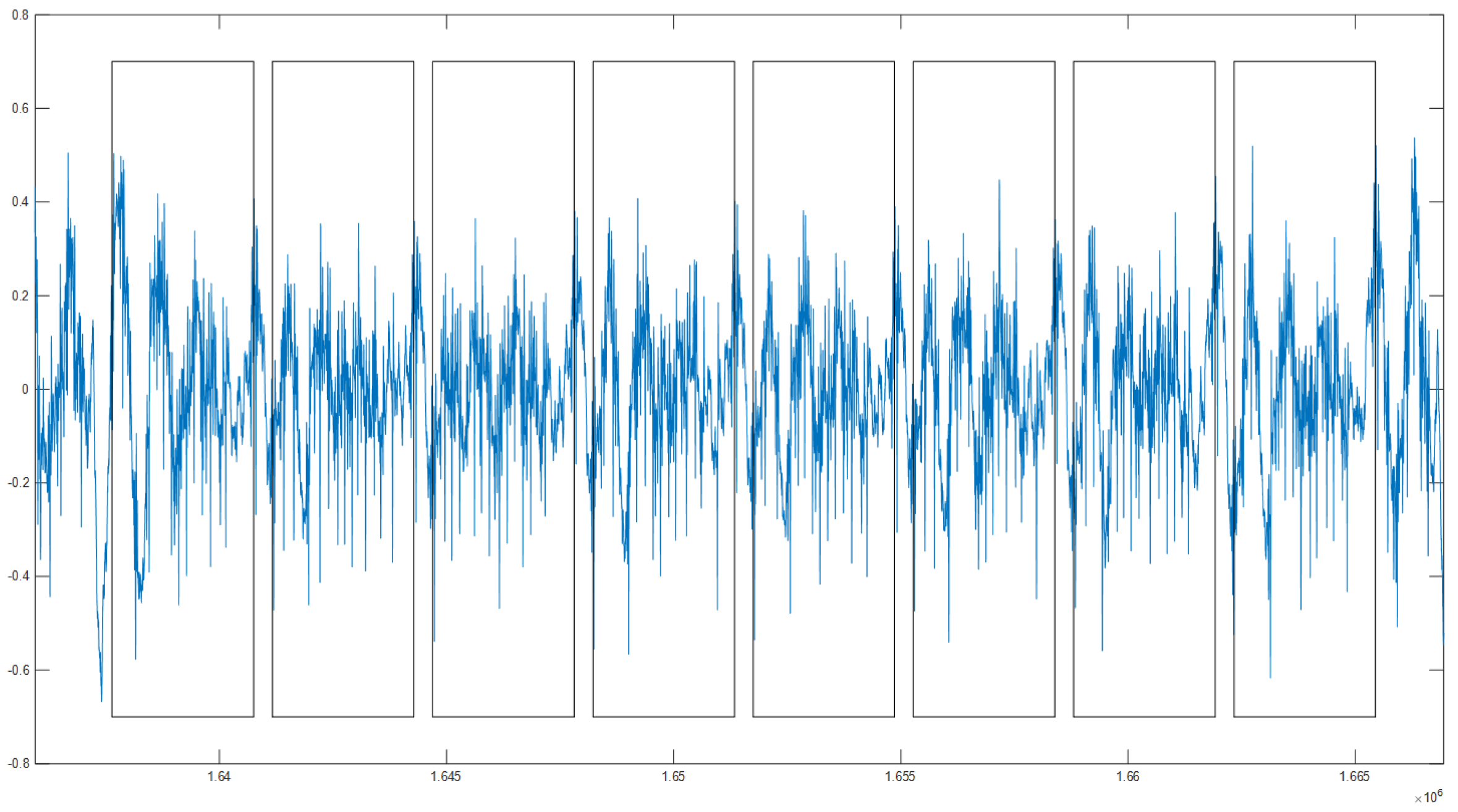
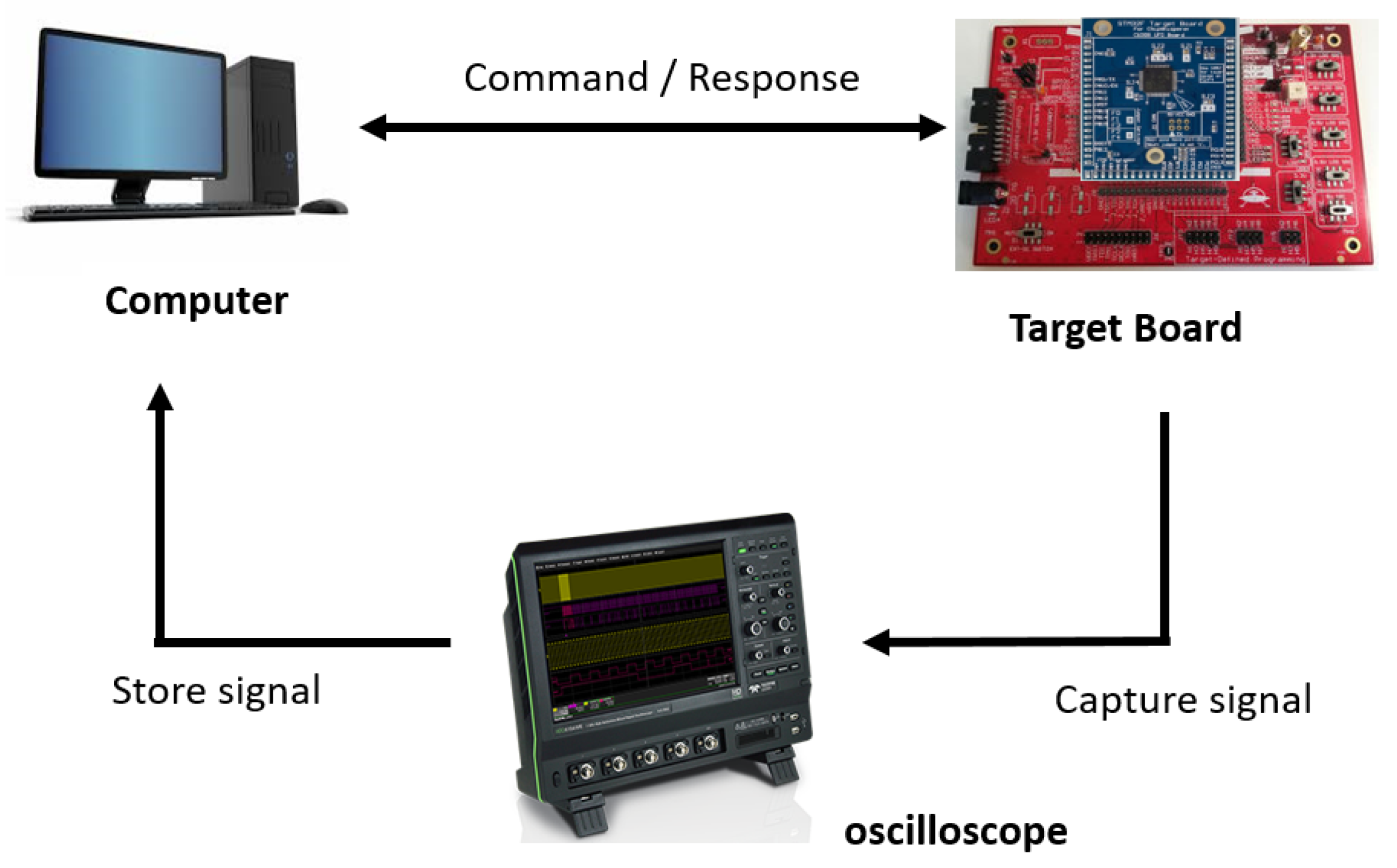
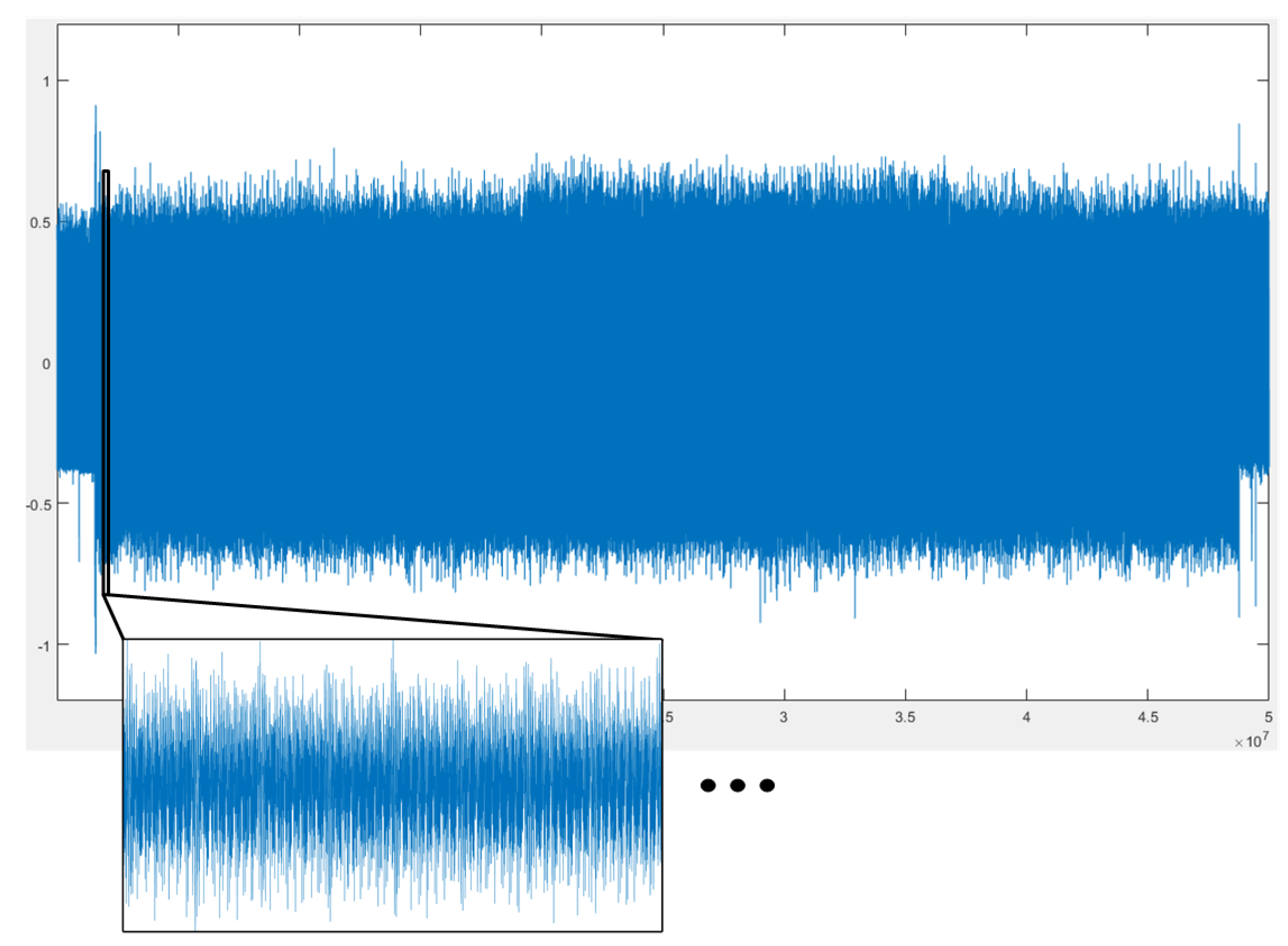
4. Experiments

In this section, we provide experimental results showing that unified point addition on the binary Huff curve is vulnerable to HCCA and ROSETTA. For this, we implemented a field multiplication for unified point addition on the binary Huff curve on an ARM cortex-m4 processor on the ChipWhisperer CW308 UFO evaluation board [12]. The scheme of the experimental setup used for measuring the power consumption is shown in Figure 1.

We collected a power consumption trace which is measured when 192 field multiplications are performed. We randomly selected whether the two operands of the two multiplications of each pair are identical or not for HCCA. Also, we randomly selected whether the operands of the multiplication are identical or not for ROSETTA. The power consumption trace was acquired using a Lecroy HDO oscilloscope with a sampling rate of 5 GS/s. We preprocessed the power consumption trace with a 168 MHz low-pass filter and 3-point maximum compression only for ROSETTA. Figure 2 shows a power consumption trace of field multiplications for unified point addition on the binary Huff curve. Using SPA and a cross-correlation technique, we identified each w-bit multiplication in a field multiplication and separated these into subtraces which correspond to each w-bit multiplication, as shown in Figure 3. For the experiment, we divided them into 96 pairs of subtraces of field multiplications for $\left(x_1\right)·\left(y_1\right)$ and $\left(x_2\right)·\left(y_2\right)$ for HCCA. Similarly, we separated a power consumption trace into subtraces of 192 field multiplications for $\left(x\right)·\left(y\right)$ for ROSETTA. To perform HCCA and ROSETTA, each subtrace was classified into two groups appropriately according to each analysis method. To find a pairwise collision, we separated the subtraces into two groups based on the following fact. Since HCCA determines whether a collision occurs during two field multiplications or not, we divided the subtraces of the w-bit multiplications ${\left(x_1\right)}_i·{\left(y_1\right)}_j$ and ${\left(x_2\right)}_i·{\left(y_2\right)}_j$ for all $i,j$ of the two multiplications $\left(x_1\right)·\left(y_1\right)$ and $\left(x_2\right)·\left(y_2\right)$ into each group. In the case of ROSETTA, similar to HCCA, we divided the subtraces of the w-bit multiplications ${\left(x\right)}_i·{\left(y\right)}_j$ and ${\left(x\right)}_j·{\left(y\right)}_i$ for all $i\ne j$ of a field multiplication $x·y$ into each group.

To find points of interest (POIs), i.e., those having the most collision-related leakage information, we calculated the sum of squared pairwise t-differences (SOST), which is Welch’s t-test of two groups, using the following:

$${\left(\frac{m_1-m_2}{\sqrt{\frac{{\sigma }_1^2}{n_1}+\frac{{\sigma }_2^2}{n_2}}}\right)}^2$$

(3)

where $m_i$ is the mean trace of group i, and ${\sigma }_i^2$ is the variance trace of group i[13,14]. SOST is a tool mainly used to identify side-channel leakage and is discussed in the SCA literature [15,16,17]. Because SOST is computed depending on the group’s statistics and each group is separated based on the operand of w-bit multiplication, points having high SOST indicate POIs. Since HCCA uses both the inputs and the output of w-bit multiplication, we selected points having a SOST value higher than some heuristic threshold. However, ROSETTA uses the output of w-bit multiplication, and we selected points having leakage of manipulating the output, considering the sequence of the multiplication. The SOST results and POIs for HCCA and ROSETTA are shown in Figure 4a,b, respectively.

We checked for a collision between subtraces corresponding to each group. The occurrence of a collision was determined by calculating Pearson’s correlation coefficients. For this, we reconstructed all subtraces composed of values of POIs only. Then, Pearson’s correlation coefficients were calculated between subtraces corresponding to each group over every point. Then, correlation coefficients corresponding to the same field multiplications and the same groups were averaged over the points. The values of the correlation coefficient sequences indicating a collision were averaged. As a result, this averaged value became a criterion for determining whether a collision occurs or not. We set the threshold by averaging all final values, which were the criteria for each collision check, and confirmed collisions by comparing the magnitude of each value and threshold. If a value was higher than the threshold, we guessed that collision occurs; otherwise, the collision was assumed not to occur. The analysis results of HCCA and ROSETTA are shown in Figure 5a,b, respectively. As a result, the success rates of HCCA and ROSETTA are 97.92% and 94.79%, respectively. These results prove that the aforementioned HCCA and ROSETTA vulnerabilities are real.

5. Countermeasures

5.1. Countermeasures

As for the two types of vulnerabilities considered in this paper, we introduce the following interesting properties: they make use of a single power consumption trace, yet they do not require knowledge of the inputs to the unified point addition formula for the binary Huff curve. Due to these properties, the application of classical blinding countermeasures (point blinding, scalar blinding, random projective coordinates) is not recommended. We propose new countermeasures against these vulnerabilities of unified point addition.

Type 1 and Type 2 vulnerabilities are due to two problems in unified point addition on the binary Huff curve. The first is that each coordinate of input points of the unified point addition operation has the same value. This problem can be solved by using the equivalence class of projective coordinates [18]. Let $\mathbb{F}$ be a finite field. In a binary Huff curve, the equivalence class containing $(X,Y,Z)$ is

$$(X:Y:Z)=\left\{\right(rX,rY,rZ):r\in \mathbb{F}\}.$$

(4)

Notice that if $(X^{\prime },Y^{\prime },Z^{\prime })\in (X:Y:Z)$, then $(X^{\prime }:Y^{\prime }:Z^{\prime })=(X:Y:Z)$. Let $P=(X:Y:Z)$ and $P^{\prime }=(X^{\prime }:Y^{\prime }:Z^{\prime })$ be the equivalence class, where $X^{\prime }=rX,Y^{\prime }=rY$, and $Z^{\prime }=rZ$, $r\ne 1$. Then, $(X:Y:Z)=(X^{\prime }:Y^{\prime }:Z^{\prime })$. When considering $P_3=P+P^{\prime }$ and $P_4=P+P$, each coordinate of input points of P and $P^{\prime }$ has a different value, but $P_3=P_4$. The equivalence class has been used in random projective coordinates (RPCs), which is a countermeasure of DPA [19]. However, RPCs are generally applied only to the input P of the elliptic curve scalar multiplication. Of course, RPCs can be applied to every execution or after each unified point addition. Unfortunately, in this case, the computational cost is disadvantageously increased for RPCs. Since we only need to convert P to a different coordinate of the same equivalence class, the bit size of r need not be the same as the bit size of the finite field. Therefore, for computational efficiency, we propose a w-bit random projective coordinate (wRPC) that limits the size of r to w bits. The proposed wRPC for the binary Huff curve is depicted in Algorithm 1.

Algorithm 1: A w-bit random projective coordinate for the binary Huff curve (wRPC)

Require: $P=(X:Y:Z)$  Ensure: $P^{\prime }=(X^{\prime }:Y^{\prime }:Z^{\prime })$ 1: Generate a w-bit random number r with $r\ne 1$ 2: $X^{\prime }\leftarrow rX;$$Y^{\prime }\leftarrow rY;$$Z^{\prime }\leftarrow rZ$ 3: return $P^{\prime }$

In Algorithm 1, w is the bit size of a word multiplication for a field multiplication. In this work, we only considered the application of wRPC on a side-channel atomic algorithm using unified point addition [4]. The side-channel atomic algorithm using wRPC is described by Algorithm 2. We show the additional cost of Algorithm 2 in Section 5.

Algorithm 2: Side-channel atomic algorithm using wRPC

Require: $P=(X:Y:Z)$, $k={(k_{n-1}...k_0)}_2$  Ensure: $kP$ 1: $R_0\leftarrow O;$$R_1\leftarrow P;$$R_2\leftarrow O;$$i\leftarrow n-1;$ 2: $k^{\prime }\leftarrow 0$ 3: while $(i\ge 1)$ do 4:    $R_0\leftarrow wRPC\left(R_2\right)$ 5:    $R_1\leftarrow wRPC\left(R_1\right)$ 6:    $R_2\leftarrow R_2+R_{k^{\prime }}$ 7:    $k^{\prime }\leftarrow k^{\prime }⨁k_i$ 8:    $i\leftarrow i-\neg k$ 9: end while 10: return $R_0$

Although Algorithm 2 using unified point addition is secure against Type 1 vulnerabilities, it is still insecure against Type 2. We show in the next subsection that it is not secure against Type 2 vulnerabilities. To be secure against Type 2 vulnerabilities, it is necessary to reconstruct the calculation process of unified point addition. For this reason, we propose a new unified point addition formula for the binary Huff curve as follows:

$m_1=X_1{X}_2,$  $m_2=Y_1{Y}_2,$  $m_3=Z_1{Z}_2,$

$m_4=(X_1+Z_1)(X_2+Z_2),$  $m_5=(Y_1+Z_1)(Y_2+Z_2),$

$m_6=m_1{m}_3,$  $m_7=m_2{m}_3,$  $m_8=m_1{m}_2+m_3^2,$

$m_9=m_6{(m_2+m_3)}^2,$  $m_{10}=m_7{(m_1+m_3)}^2,$  $m_{11}=m_8(m_2+m_3),$

$m_{12}=m_8(m_1+m_3),$

$Z_3=m_{11}(m_1+m_3),$

$X_3=(m_4+m_{11})m_{11}+m_{11}^2+\alpha m_9+Z_3,$

$Y_3=(m_5+m_{12})m_{12}+m_{12}^2+\beta m_{10}+Z_3.$

The proposed unified point addition operation is based on masking by $m_4$ and $m_5$. To use the advantage of almost no computational cost for squaring in a binary field, we configured the calculation of masking $m_4$ and $m_5$ by squaring. Thus, the proposed method needs 17 field multiplications, which is exactly the same as in [9]. Furthermore, we explain Type 1 and Type 2 vulnerabilities of several unified point addition formulae and propose countermeasures in the Appendix A.

5.2. Security Analysis of the Proposed Method

In this section, we analyze Type 1 and Type 2 vulnerabilities of Algorithm 2 using the proposed unified point addition method. Let the input $R_2=(X_1:Y_1:Z_1)$ in step 4 and let the input $R_1=(X_2:Y_2:Z_2)$ in step 5. Then, in step 6, the two inputs $R_2$ and $R_{k^{\prime }}$ of the proposed unified point addition are $P_1=R_2,$ $P_2=R_0$ if $k^{\prime }=0$ and $P_1=R_2,$ $P_2=R_1$ if $k^{\prime }=1$. The two inputs are expressed as follows:

$$\left\{\begin{array}{cc}{P}_1=(X_1:Y_1:Z_1),P_2=(r_1{X}_1:r_1{Y}_1:r_1{Z}_1)\hfill & \mathrm{If}{k}^{\prime }=0,\hfill \\ P_1=(X_1:Y_1:Z_1),P_2=(r_2{X}_2:r_2{Y}_2:r_2{Z}_2)\hfill & \mathrm{If}{k}^{\prime }=1.\hfill \end{array}\right.$$

(5)

where $r\ne 1$. The proposed unified point addition method can be evaluated as shown in

Table 2. The proposed unified point addition method on the binary Huff curve in Algorithm 2.

Out	${\mathit{P}}_1={\mathit{P}}_2({\mathit{k}}^{\prime }=0)$	${\mathit{P}}_1\ne {\mathit{P}}_2({\mathit{k}}^{\prime }=1)$
$m_1$	$\left[X_1\right]·\left[r_1{X}_1\right]$	$\left[X_1\right]·\left[r_2{X}_2\right]$
$m_2$	$\left[Y_1\right]·\left[r_1{Y}_1\right]$	$\left[Y_1\right]·\left[r_2{Y}_2\right]$
$m_3$	$\left[Z_1\right]·\left[r_1{Z}_1\right]$	$\left[Z_1\right]·\left[r_2{Z}_2\right]$
$m_4$	$\left[(X_1+Z_1)\right]·\left[(r_1{X}_1+r_1{Z}_1)\right]$	$\left[(X_1+Z_1)\right]·\left[(r_2{X}_2+r_2{Z}_2)\right]$
$m_5$	$\left[(Y_1+Z_1)\right]·\left[(r_1{Y}_1+r_1{Z}_1)\right]$	$\left[(Y_1+Z_1)\right]·\left[(r_2{Y}_2+r_2{Z}_2)\right]$
$m_6=m_1·m_3$	$\left[r_1{X}_1^2\right]·\left[r_1{Z}_1^2\right]$	$\left[r_2{X}_1{X}_2\right]·\left[r_2{Z}_1{Z}_2\right]$
$m_7=m_2·m_3$	$\left[r_1{Y}_1^2\right]·\left[r_1{Z}_1^2\right]$	$\left[r_2{Y}_1{Y}_2\right]·\left[r_2{Z}_1{Z}_2\right]$
$m_8=m_1·m_2+m_3^2$	$\left[r_1{X}_1^2\right]·\left[r_1{Y}_1^2\right]+{\left(r_1{Z}_1^2\right)}^2$	$\left[r_2{X}_1{X}_2\right]·\left[r_2{Y}_1{Y}_2\right]+{\left(r_2{Z}_1{Z}_2\right)}^2$
$m_9=m_6·{(m_2+m_3)}^2$	$\left[r_1^2{X}_1^2{Z}_1^2\right]·\left[{(r_1{Y}_1^2+r_1{Z}_1^2)}^2\right]$	$\left[r_2^2{X}_1{X}_2{Z}_1{Z}_2\right]·\left[{(r_2{Y}_1{Y}_2+r_2{Z}_1{Z}_2)}^2\right]$
$m_{10}=m_7·{(m_1+m_3)}^2$	$\left[r_1^2{Y}_1^2{Z}_1^2\right]·\left[{(r_1{X}_1^2+r_1{Z}_1^2)}^2\right]$	$\left[r_2^2{Y}_1{Y}_2{Z}_1{Z}_2\right]·\left[{(r_2{X}_1{X}_2+r_2{Z}_1{Z}_2)}^2\right]$
$m_{11}=m_8·(m_2+m_3)$	$\left[r_1^2(X_1^2{Y}_1^2+Z_1^4)\right]·\left[r_1(Y_1^2+Z_1^2)\right]$	$\left[r_2^2(X_1{X}_2{Y}_1{Y}_2+{\left(Z_1{Z}_2\right)}^2)\right]·\left[r_2(Y_1{Y}_2+Z_1{Z}_2)\right]$
$m_{12}=m_8·(m_1+m_3)$	$\left[r_1^2(X_1^2{Y}_1^2+Z_1^4)\right]·\left[r_1(X_1^2+Z_1^2)\right]$	$\left[r_2^2(X_1{X}_2{Y}_1{Y}_2+{\left(Z_1{Z}_2\right)}^2)\right]·\left[r_2(X_1{X}_2+Z_1{Z}_2)\right]$
$Z_3^{\prime }=m_{11}·(m_1+m_3)$	$\left[r_1^3(X_1^2{Y}_1^2+Z_1^4)(Y_1^2+Z_1^2)\right]·\left[r_1(X_1^2+Z_1^2)\right]$	$\left[r_2^3(X_1{X}_2{Y}_1{Y}_2+{\left(Z_1{Z}_2\right)}^2)(Y_1{Y}_2+Z_1{Z}_2)\right]·\left[r_2(X_1{X}_2+Z_1{Z}_2)\right]$
$X_3^{\prime }=(m_4+m_{11})·m_{11}+m_{11}^2+\alpha ·m_9+Z_3$	$[r_1(X_1^2+Z_1^2)·\left[r_1^3(X_1^2{Y}_1^2+Z_1^4)(Y_1^2+Z_1^2)\right]+r_1^3(X_1^2{Y}_1^2+Z_1^4)(Y_1^2+Z_1^2)]+{\left(r_1^3(X_1^2{Y}_1^2+Z_1^4)(Y_1^2+Z_1^2)\right)}^2+\left[\alpha \right]·\left[r_1^4{X}_1^2{Z}_1^2{(Y_1^2+Z_1^2)}^2\right]+Z_3$	$[r_2(X_1+Z_1)(X_2+Z_2)+r_2^3(X_1{X}_2{Y}_1{Y}_2+{\left(Z_1{Z}_2\right)}^2)(Y_1{Y}_2+Z_1{Z}_2)]·\left[r_2^3(X_1{X}_2{Y}_1{Y}_2+{\left(Z_1{Z}_2\right)}^2)(Y_1{Y}_2+Z_1{Z}_2)\right]+\left[\alpha \right]·\left[r_2^4{X}_1{X}_2{Z}_1{Z}_2{(Y_1{Y}_2+Z_1{Z}_2)}^2\right]+Z_3$
$Y_3^{\prime }=(m_5+m_{12})·m_{12}+m_{12}^2+\beta ·m_{10}+Z_3$	$[r_1(Y_1^2+Z_1^2)+r_1^3(X_1^2{Y}_1^2+Z_1^4)(X_1^2+Z_1^2)]·\left[r_1^3(X_1^2{Y}_1^2+Z_1^4)(X_1^2+Z_1^2)\right]+{\left(r_1^3(X_1^2{Y}_1^2+Z_1^4)(X_1^2+Z_1^2)\right)}^2+\left[\beta \right]·\left[r_1^4{Y}_1^2{Z}_1^2{(X_1^2+Z_1^2)}^2\right]+Z_3$	$[r_2(Y_1+Z_1)(Y_2+Z_2)+r_2^3(X_1{X}_2{Y}_1{Y}_2+{\left(Z_1{Z}_2\right)}^2)(X_1{X}_2+Z_1{Z}_2)]·\left[r_2^3(X_1{X}_2{Y}_1{Y}_2+{\left(Z_1{Z}_2\right)}^2)(X_1{X}_2+Z_1{Z}_2)\right]+{\left(r_2^3(X_1{X}_2{Y}_1{Y}_2+{\left(Z_1{Z}_2\right)}^2)(X_1{X}_2+Z_1{Z}_2)\right)}^2+\left[\beta \right]·\left[r_2^4{Y}_1{Y}_2{Z}_1{Z}_2{(X_1{X}_2+Z_1{Z}_2)}^2\right]+Z_3$

.

• Type 1 vulnerability: As shown in Table 2, if $P_1=P_2(k^{\prime }=0)$, then the output of the proposed unified point addition operation is $X_3^{\prime }=r_1^4{X}_3,Y_3^{\prime }=r_1^4{Y}_3,Z_3^{\prime }=r_1^4{Z}_3$, where $(X_3:Y_3:Z_3)$ is the output of Table 1. Since $(X_3^{\prime },Y_3^{\prime },Z_3^{\prime })\in (X_3,Y_3,Z_3)$, then $(X_3^{\prime },Y_3^{\prime },Z_3^{\prime })=(X_3:Y_3:Z_3)$. In addition, if $P_1=P_2$, then $m_1,m_2,m_3,m_4$, and $m_5$ can be computed as follows:
  $m_1=\left(X_1\right)\left(r_1{X}_1\right),$  $m_2=\left(Y_1\right)\left(r_1{Y}_1\right),$  $m_3=\left(Z_1\right)\left(r_1{Z}_1\right),$
  $m_4=(X_1+Z_1)(r_1{X}_1+r_1{Z}_1),$  $m_5=(Y_1+Z_1)(r_1{Y}_1+r_1{Z}_1).$
  For $m_1$, although $P_1=P_2$, the operands $X_1$ and $r_1{X}_1$ are different. Similarly, the operands of the field multiplications for $m_2,m_3,m_4$, and $m_5$ are different. Also, there is no other field multiplication vulnerable to Type 1. Thus, the proposed algorithm is secure against the Type 1 vulnerability for the binary Huff curve.
• Type 2 vulnerability: Although wRPC is applied to the proposed unified point addition operation, $m_4=\left[(X_1+Z_1)\right]·\left[(r_1{X}_1+r_1{Z}_1)\right]=r_1(X_1{X}_1+Z_1{Z}_1)$ and $m_1+m_3=r_1{X}_1{X}_1+r_1{Z}_1{Z}_1$ when $P_1=P_2(k^{\prime }=0)$. Thus, $m_4=m_1+m_3$. Similarly, $m_5{m}_8=m_{11}$. Thus, if we compute $\left[m_{11}\right]·\left[(m_1+m_3)\right]$, $\left[m_4\right]·\left[m_{11}\right]$, and $\left[m_5{m}_8\right]·\left[(m_1+m_3)\right]$ as the previous unified point addition operation, their operands are the same when $P_1=P_2$. On the other hand, they are different when $P_1\ne P_2$. Likewise, the operands of $\left[m_8\right]·\left[(m_2+m_3)\right]$ and $\left[m_5\right]·\left[m_8\right]$ are the same when $P_1=P_2$. They become targets to a Type 2 vulnerability. The reason for this vulnerability is that the same intermediate results occur in the previous unified point addition operation. They are used as inputs to more than one multiplication without modification for $P_1=P_2$. Thus, we used the proposed method to mask the operands of vulnerable multiplications. Considering $\left[m_4\right]·\left[m_{11}\right]$ and $\left[m_{11}\right]·\left[(m_1+m_3)\right]$ in Table 1, since the operand $m_{11}$ is identically used in two multiplications, they do not affect the vulnerability. Thus, we only have to mask the other operand $m_4$ (or $m_1+m_3$). Specifically, we computed $\left[m_4\right]·\left[m_{11}\right]$ as $\left[(m_4+M)\right]·\left[m_{11}\right]+M·m_{11}$ so that an adversary cannot distinguish between $P_1=P_2$ and $P_1\ne P_2$ using a Type 2 vulnerability. However, we additional cost is incurred for $M·m_{11}$. To reduce this additional cost, we computed $\left[m_4\right]·\left[m_{11}\right]$ as $\left[(m_4+m_{11})\right]·\left[m_{11}\right]+m_{11}^2$ to use the advantage of zero computational cost for squaring in a binary field, which is almost free. Similarly, we applied masking to $\left[m_5\right]·\left[m_{12}\right]$ as $\left[(m_5+m_{12})\right]·\left[m_{12}\right]+m_{12}^2$. In addition, for $\left[m_8\right]·\left[(m_2+m_3)\right]$ and $\left[m_5\right]·\left[m_8\right]$, we modified the computation of $Y_3$ as $m_{12}=m_8(m_1+m_3)$ and $Y_3=(m_5+m_{12})m_{12}+m_{12}^2+\beta m_{10}+Z_3$ without performing $\left[m_5\right]·\left[m_8\right]$. Based on the proposed algorithm, Type 1 and Type 2 vulnerabilities no longer exist (Table 2).

6. Comparisons

We compared the proposed method with the previously presented unified point addition operations with respect to computational cost. Also, we compared the proposed method with the previously unified point addition formulae to which we applied the blinding operands of field multiplication. In this work, as the side-channel atomic algorithms, we considered (i) the proposed method, (ii) the unified point additions in [8,9], and (iii) the application of the blinding operands of a field multiplication [10] on the unified point addition method in [8,9]. We analyzed two aspects, that is, security against SCAs and computational cost.

Table 3. The security against side-channel attacks (SCAs) of algorithms.

Algorithm	SPA	ROSETTA	HCCA
[8]	insecure	insecure	insecure
[9]	secure	insecure	insecure
[8] using [10]	secure	secure	secure
[9] using [10]	secure	secure	secure
proposed method	secure	secure	secure

shows the security against SCAs. The unified point additions described in [8,9] using the blinding operands in [10] are secure against ROSETTA and HCCA.

The computational costs of [8,9] are the same. Also, the computational cost of the proposed unified point addition method is the same as that of the previous one. Thus, the computational costs of the algorithms are affected by the additional cost of wRPC and [10]. Let $w=32$ and let n be the bit size of a finite field. Also, let $t=\lceil n/32\rceil$. We consider that n has one of the bit sizes of the standard binary curve in FIPS 186-3 [20] $(233,283,409$, and $571)$. The computational cost of an iteration of the algorithms is shown in

Table 4. The computational cost of the algorithms of the binary Huff curve.

n	Algorithm	M	Additional Cost	Total Cost	Ratio
233	[8,9]	64	-	1088	1.000
	[8,9] using [10]	81	-	1377	1.266
	proposed method	64	48	1136	1.044
283	[8,9]	81	-	1377	1.000
	[8,9] using [10]	100	-	1700	1.235
	proposed method	81	54	1431	1.039
409	[8,9]	169	-	2873	1.000
	[8,9] using [10]	196	-	3332	1.160
	proposed	169	78	2951	1.027
571	[8,9]	324	-	5508	1.000
	[8,9] using [10]	361	-	6137	1.114
	proposed method	324	108	5616	1.020

.

In Table 4, M is the number of w-bit multiplications of a field multiplication. Namely, $M=t^2$ in [8,9] and in the proposed method. Also, $M=t^2+2t+1$ in [8,9] with [10]. The additional cost is the number of w-bit multiplications of wRPC in the proposed method. Namely, (additional cost) $=2*(3*t)$ for the proposed method. The total cost is the number of w-bit multiplications of an iteration of the side-channel atomic algorithm using unified point additions. Namely, (total cost) $=17*M+$ (additional cost). The ratio is the overhead of the algorithm when the original algorithm [8,9] is assumed as 1. This shows that the proposed algorithm is about 0.2∼4.4% slower than [8,9]. However, the methods from [8,9] are not secure against ROSETTA and HCCA. The proposed method is about 8.5∼17.5% faster than the previous methods from [8,9] using [10], which are secure against ROSETTA and HCCA. In addition, the previous methods ([8,9] using [10]) also require random number generation for $r_1$ and $r_2$ in each field multiplication.

7. Conclusions

In this paper, we present two vulnerabilities of unified point addition on the binary Huff curve; these vulnerabilities are exploitable by ROSETTA and HCCA. In particular, we found these vulnerabilities of unified point addition on the binary Huff curve as presented in [9]. As countermeasures, we propose wRPC and present a new unified point addition method for the binary Huff curve. Additionally, we show the proposed unified point addition method and wRPC applied to the side-channel atomic algorithm. The proposed method is secure against ROSETTA and HCCA. In addition, the proposed unified point addition method has no additional cost compared to the previous one. However, wRPC does incur additional cost. Depending on the size of the base field of an elliptic curve, the proposed method is about 0.2∼4.4% slower than the original one. However, it is about 8.5∼17.5% faster than unified point additions using blinding operands as a countermeasure. Additionally, we present our analyses of the vulnerabilities of unified point addition on other elliptic curves, such as Weierstraß, Hessian, Edwards, Jacobi intersections, Jacobi quartic, and binary Edwards elliptic curves in the Appendix A.

References

- Kocher, P.; Jaffe, J.; Jun, B. Differential power analysis. In Proceedings of the Annual International Cryptology Conference, Santa Barbara, CA, USA, 15–19 August 1999; Springer: Berlin/Heidelberg, Germany, 1999; pp. 388–397. [Google Scholar]
- Coron, J.S. Resistance against differential power analysis for elliptic curve cryptosystems. In Proceedings of the International Workshop on Cryptographic Hardware and Embedded Systems, Worcester, MA, USA, 12–13 August 1999; Springer: Berlin/Heidelberg, Germany, 1999; pp. 292–302. [Google Scholar]
- Izu, T.; Takagi, T. A fast parallel elliptic curve multiplication resistant against side channel attacks. In Proceedings of the International Workshop on Public Key Cryptography, Paris, France, 12–14 February 2002; Springer: Berlin/Heidelberg, Germany, 2002; pp. 280–296. [Google Scholar]
- Chevallier-Mames, B.; Ciet, M.; Joye, M. Low-cost solutions for preventing simple side-channel analysis: Side-channel atomicity. IEEE Trans. Comput. 2004, 53, 760–768. [Google Scholar] [CrossRef]
- Brier, E.; Joye, M. Weierstraß elliptic curves and side-channel attacks. In Proceedings of the International Workshop on Public Key Cryptography, Paris, France, 12–14 February 2002; Springer: Berlin/Heidelberg, Germany, 2002; pp. 335–345. [Google Scholar]
- Bauer, A.; Jaulmes, E.; Prouff, E.; Reinhard, J.R.; Wild, J. Horizontal collision correlation attack on elliptic curves. Cryptogr. Commun. 2015, 7, 91–119. [Google Scholar] [CrossRef]
- Clavier, C.; Feix, B.; Gagnerot, G.; Giraud, C.; Roussellet, M.; Verneuil, V. ROSETTA for single trace analysis. In Proceedings of the International Conference on Cryptology in India, Kolkata, India, 9–12 December 2012; Springer: Berlin/Heidelberg, Germany, 2012; pp. 140–155. [Google Scholar]
- Devigne, J.; Joye, M. Binary huff curves. In Proceedings of the Cryptographers’ Track at the RSA Conference, San Francisco, CA, USA, 14–18 February 2011; Springer: Berlin/Heidelberg, Germany, 2011; pp. 340–355. [Google Scholar]
- Ghosh, S.; Kumar, A.; Das, A.; Verbauwhede, I. On the implementation of unified arithmetic on binary huff curves. In Proceedings of the International Workshop on Cryptographic Hardware and Embedded Systems, Santa Barbara, CA, USA, 20–23 August 2013; Springer: Berlin/Heidelberg, Germany, 2013; pp. 349–364. [Google Scholar]
- Clavier, C.; Feix, B.; Gagnerot, G.; Roussellet, M.; Verneuil, V. Horizontal correlation analysis on exponentiation. In Proceedings of the International Conference on Information and Communications Security, Barcelona, Spain, 15–17 December 2010; Springer: Berlin/Heidelberg, Germany, 2010; pp. 46–61. [Google Scholar]
- Joye, M.; Tibouchi, M.; Vergnaud, D. Huff’s model for elliptic curves. In Proceedings of the International Algorithmic Number Theory Symposium, Nancy, France, 19–23 July 2010; Springer: Berlin/Heidelberg, Germany, 2010; pp. 234–250. [Google Scholar]
- O’Flynn, C.; Chen, Z.D. Chipwhisperer: An open-source platform for hardware embedded security research. In Proceedings of the International Workshop on Constructive Side-Channel Analysis and Secure Design, Paris, France, 13–15 April 2014; Springer: Berlin/Heidelberg, Germany, 2014; pp. 243–260. [Google Scholar]
- Gierlichs, B.; Lemke-Rust, K.; Paar, C. Templates vs. stochastic methods. In Proceedings of the International Workshop on Cryptographic Hardware and Embedded Systems, Yokohama, Japan, 10–13 October 2006; Springer: Berlin/Heidelberg, Germany, 2006; pp. 15–29. [Google Scholar]
- Welch, B.L. The generalization ofstudent’s’ problem when several different population variances are involved. Biometrika 1947, 34, 28–35. [Google Scholar] [PubMed]
- Hospodar, G.; Gierlichs, B.; De Mulder, E.; Verbauwhede, I.; Vandewalle, J. Machine learning in side-channel analysis: a first study. J. Cryptogr. Eng. 2011, 1, 293. [Google Scholar] [CrossRef]
- Choudary, O.; Kuhn, M.G. Efficient template attacks. In Proceedings of the International Conference on Smart Card Research and Advanced Applications, Berlin, Germany, 27–29 November 2013; Springer: Berlin/Heidelberg, Germany, 2013; pp. 253–270. [Google Scholar]
- Durvaux, F.; Standaert, F.X. From improved leakage detection to the detection of points of interests in leakage traces. In Proceedings of the Annual International Conference on the Theory and Applications of Cryptographic Techniques, Vienna, Austria, 8–12 May 2016; Springer: Berlin/Heidelberg, Germany, 2016; pp. 240–262. [Google Scholar]
- Hankerson, D.; Menezes, A.J.; Vanstone, S. Guide to Elliptic Curve Cryptography; Springer Science & Business Media: Berlin/Heidelberg, Germany, 2006. [Google Scholar]
- Fan, J.; Guo, X.; De Mulder, E.; Schaumont, P.; Preneel, B.; Verbauwhede, I. State-of-the-art of secure ECC implementations: a survey on known side-channel attacks and countermeasures. In Proceedings of the 2010 IEEE International Symposium on Hardware-Oriented Security and Trust (HOST), Anaheim, CA, USA, 13–14 June 2010; pp. 76–87. [Google Scholar]
- Locke, G.; Gallagher, P. Fips pub 186-3: Digital signature standard (dss). Fed. Inf. Process. Stand. Publ. 2009, 3, 186-3. [Google Scholar]
- Bernstein, D.J. Explicit-Formulas Database. Available online: http://www. hyperelliptic. org/EFD (accessed on 22 October 2018).