A Hybrid Forecasting Method for Solar Output Power Based on Variational Mode Decomposition, Deep Belief Networks and Auto-Regressive Moving Average

Abstract

Due to the existing large-scale grid-connected photovoltaic (PV) power generation installations, accurate PV power forecasting is critical to the safe and economical operation of electric power systems. In this study, a hybrid short-term forecasting method based on the Variational Mode Decomposition (VMD) technique, the Deep Belief Network (DBN) and the Auto-Regressive Moving Average Model (ARMA) is proposed to deal with the problem of forecasting accuracy. The DBN model combines a forward unsupervised greedy layer-by-layer training algorithm with a reverse Back-Projection (BP) fine-tuning algorithm, making full use of feature extraction advantages of the deep architecture and showing good performance in generalized predictive analysis. To better analyze the time series of historical data, VMD decomposes time series data into an ensemble of components with different frequencies; this improves the shortcomings of decomposition from Empirical Mode Decomposition (EMD) and Ensemble Empirical Mode Decomposition (EEMD) processes. Classification is achieved via the spectrum characteristics of modal components, the high-frequency Intrinsic Mode Functions (IMFs) components are predicted using the DBN, and the low-frequency IMFs components are predicted using the ARMA. Eventually, the forecasting result is generated by reconstructing the predicted component values. To demonstrate the effectiveness of the proposed method, it is tested based on the practical information of PV power generation data from a real case study in Yunnan. The proposed approach is compared, respectively, with the single prediction models and the decomposition-combined prediction models. The evaluation of the forecasting performance is carried out with the normalized absolute average error, normalized root-mean-square error and Hill inequality coefficient; the results are subsequently compared with real-world scenarios. The proposed approach outperforms the single prediction models and the combined forecasting methods, demonstrating its favorable accuracy and reliability.

1. Introduction

To promote sustainable economic and social development, energy sources such as solar energy and wind power need to be leveraged to counteract the rapidly growing energy consumption and deteriorating environment caused by climate change. To promote increased solar energy utilization, photovoltaic (PV) power generation has been rapidly developed worldwide [1]. PV power generation is affected by solar radiation, temperature and other factors. It also has strong intermittency and volatility. Grid access by large-scale distributed PV power introduces significant obstacles to the planning, operation, scheduling and control of power systems. Accurate PV power prediction not only provides the basis for grid dispatch decision-making behavior, but also provides support for multiple power source space-time complementarity and coordinated control; this reduces pre-existing rotating reserve capacity and operating costs, which ensures the safety and stability of the system and promotes the optimal operation of the power grid [2].

According to the timescale, PV power forecasting can be divided into long-term, short-term, and ultra-short-term forecasts [3]. A medium-long-term forecast (i.e., with a prediction scale of several months) can provide support for power grid planning; Short-term prediction (i.e., with a prediction scale of one to four days in advance) can assist the dispatching department in formulating generator set start-stop plans. Super short-term forecast (i.e., with a prediction scale of 15 min in advance) can achieve a real-time rolling correction of the output plan curve and can provide early warning information to the dispatcher. The shorter the time scale, the more favorable the management of preventative situations and emergencies. Most of the existing literature describes short-term forecasting research with an hourly cycle. There are few reports on the ultra-short-term prediction of PV power generation [4,5,6]. In addition, in the previous research, PV power prediction methods mainly include the following: physical methods, statistical methods, machine learning methods, and hybrid integration methods.

(1) In physical methods, numerical weather prediction (NWP) is the most widely used method, which involves more input data such as solar radiation, temperature, and other meteorological information.

(2) As for the statistical approaches, their main purpose is to establish a long-term PV output prediction model. In literature [7,8,9,10], the auto-regressive, auto-regressive moving average, auto-regressive integral moving average and Kalman filtering model of short-term PV prediction are respectively established based on the time series, and obtain good prediction results. The above model is mainly based on a linear model, which only requires historical PV data and does not require more meteorological factors. In addition, the time series methods can only capture linear relationships and require stationary input data or stationary differencing data.

(3) Along with the rapid update of computer hardware and the development of data mining, prediction methods based on machine learning have been successfully applied in many fields. Machine learning models that have been widely applied in PV output prediction models are nonlinear regression models such as the Deep Neural Network (DNN), the Recurrent Neural Network (RNN), the Convolutional Neural Network (CNN), the Deep Belief Network (DBN) and so forth. Literature [11,12] establishes output prediction models based on the neural network, which can consider multiple input influencing factors at the same time. The only drawback is that the network structure and parameter settings will have a great impact on the performance of the models, which limits the application of neural networks. Literature [13,14] has analyzed various factors affecting PV power and established support vector machine (SVM) prediction models facing PV prediction. The results show that the SVM adopts the principle of structural risk minimization to replace the principle of empirical risk minimization of traditional neural networks; thus, it has a better generalization ability. To effectively enhance the reliability and accuracy of PV prediction results, related literature proposes the use of intelligent optimization algorithms to estimate model parameters; some examples of intelligent optimization algorithms include the gray wolf algorithm, the similar day analysis method and the particle swarm algorithm [15,16,17]. The example analysis illustrates the effectiveness of the optimization algorithm.

(4) In recent years, decomposition-refactoring prediction models based on signal analysis methods have attracted more and more attention from scholars. Relevant research shows that using signal analysis methods to preprocess data on PV power series can reduce the influence of non-stationary meteorological external factors on the prediction results and improve prediction accuracy. The decomposition methods of PV power output data mainly include wavelet analysis and wavelet packet transform [18,19], empirical mode decomposition (EMD) [20], ensemble empirical mode decomposition (EEMD) [21] and local mean decomposition (LMD) [22]. Among them, wavelet analysis has good time-frequency localization characteristics, but the decomposition effect depends on the choice of basic function and the self-adaptability is poor [23]. EMD has strong self-adaptability, but there are problems such as end-effects and over-enveloping [24]. LMD has fewer iterations and lighter end-effects. However, judging the condition of purely FM signals requires trial and error. If the sliding span is not properly selected, the function will not converge, resulting in excessive smoothness, which affects algorithmic accuracy [25]. EEMD is the improved EMD method; the analysis of the signal is made via a noise-assisted, weakened influence of modal aliasing. However, this method has a large amount of computation and more modal components than the true value [26]. Variational mode decomposition (VMD) is a relatively new signal decomposition method. Compared to the recursive screening mode of EMD, EEMD, and LMD, by controlling the modal center frequency K, the VMD transforms the estimation of the sequence signal modality into a non-recursive variational modal problem to be solved, which can well express and separate the weak detail signal and the approximate signal in the signal. It is essentially a set of adaptive Wiener filters with a mature theoretical basis. In addition, the non-recursive method adopted does not transmit errors, and solves the modal aliasing phenomenon of EMD, EEDM and other methods appeared in the background of bad noise, and effectively weakens the degree of end-effect [27]. Literature [28] used this method for fault diagnoses and achieved good results.

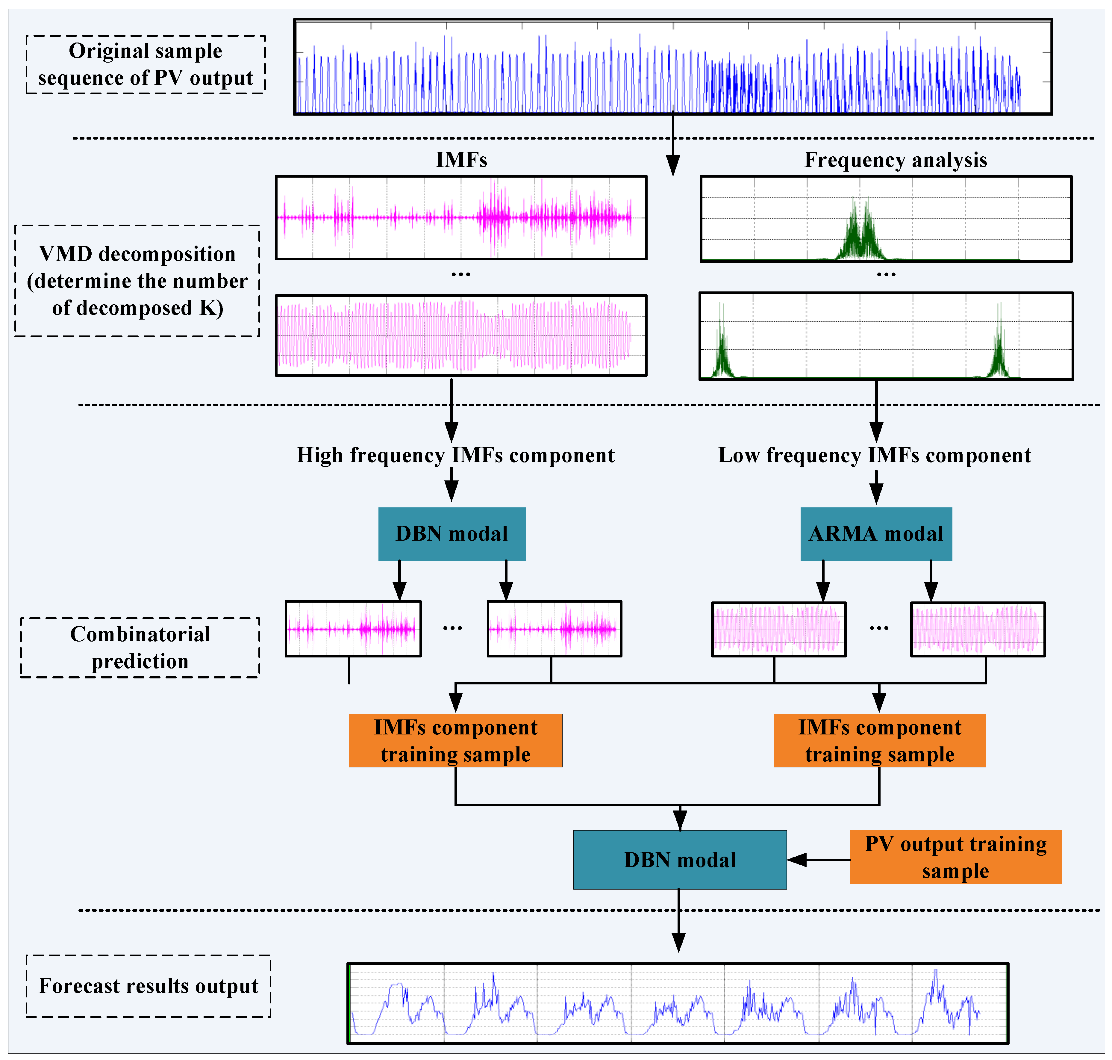
Through the above literature research, we find that the previous prediction methods using traditional neural network models and single machine learning models cannot meet the performance requirements of local solar irradiance prediction scenarios with complex fluctuations. To further improve the prediction accuracy of PV output, this work proposes a new and innovative hybrid prediction method that can improve prediction performance. This method is a hybrid of variational mode decomposition (VMD), the deep belief network (DBN), and the auto-regressive moving average model (ARMA); it combines these prediction techniques adaptively. Different from the traditional PV output prediction model, the key features of the VMD-ARMA-DBN prediction model are the perfect combination of the following parts: (1) VMD-based solar radiation sequence decomposition; (2) ARMA-based low-frequency component sequence prediction model; and (3) DBN-based high-frequency component sequence prediction model. The original photovoltaic output sequences are decomposed into multiple controllable subsequences of different frequencies by using the VMD methods. Then, based on the frequency characteristics of each subsequence, the subsequence prediction is performed by using the advantages of ARMA and DBN, respectively. Finally, the subsequences are reorganized, and the final PV output prediction value is obtained. The main contributions of this article are as follows:

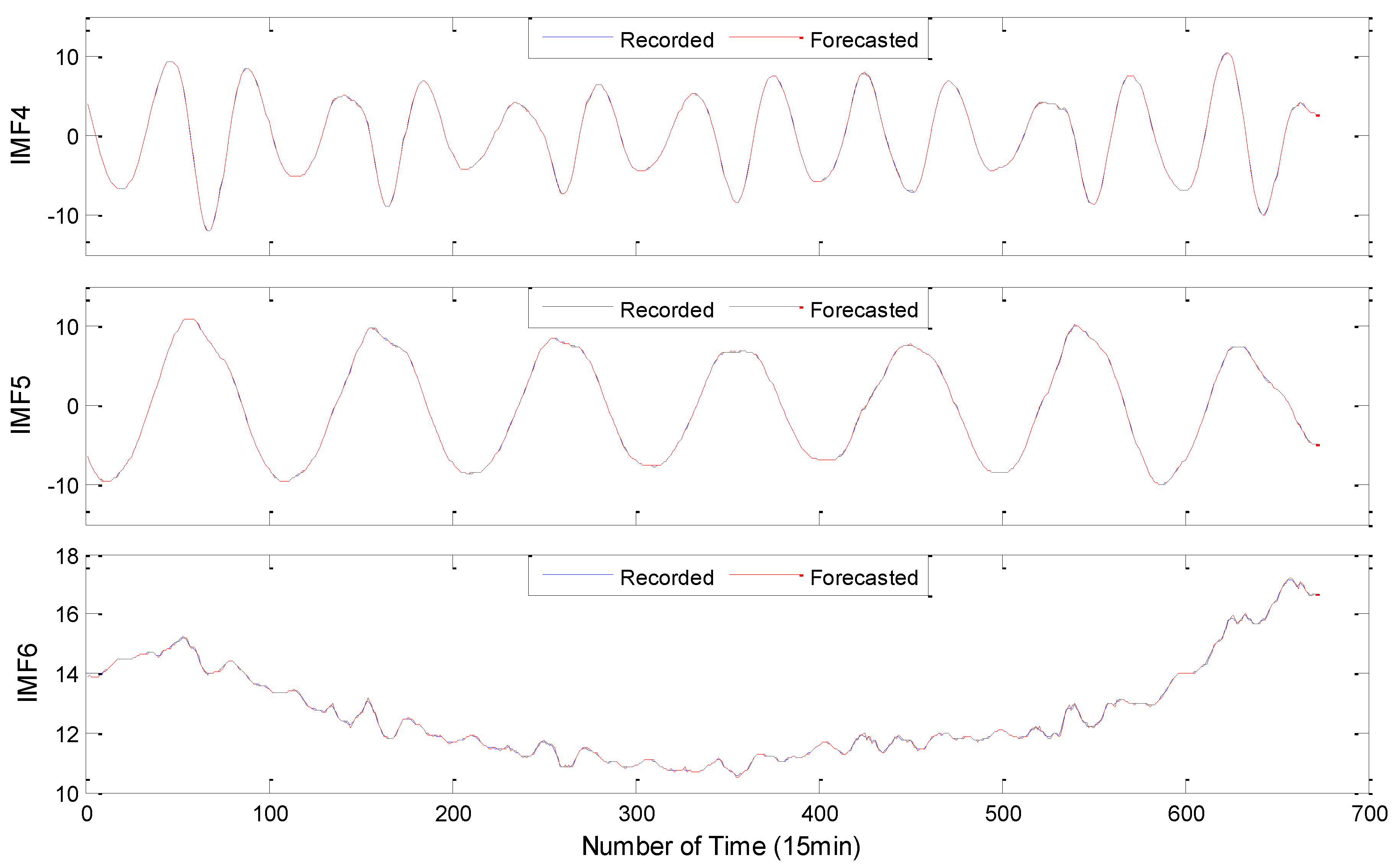
(1) To reduce the complexity and non-stationarity of the PV output data series, the VMD decomposition is used for the first time to preprocess the PV data sequence and decompose it into a series of IMF component sequences with good characteristics, achieving an effective extraction of advanced nonlinear features and hidden structures in PV output data sequences.

(2) An innovative method for predicting PV output based on VMD-DBM-ARMA is proposed. According to the characteristics of the IMF component sequence decomposed by the VMD, DBN and ARMA models are used to improve predictions of the high- and low-frequency component sequences, respectively. Based on this, the DBN is used for feature extraction and structural learning of the prediction results of each component sequence. Finally, the PV output predictive value is obtained.

(3) Taking the actual measured data of a PV power plant in China-Yunnan for application, the short-term PV output predictions of ARMA, DBN, EMD-ARMA-DBN, EEMD-ARMA-DBN, and VMD-ARMA-DBN were conducted and three prediction precisions were introduced, respectively. The evaluation indicators perform a statistical analysis on the prediction effect of each model. The results show that the proposed method can guarantee the stability of the prediction error and further improve the PV prediction accuracy.

The remainder of this paper is organized as follows: Section 2 describes our proposed approach: A Hybrid Forecasting Method for Solar Output Power Based on VMD-DBN-ARMA; experimental results are presented in Section 3; and the experimental comparison and conclusion are given in Section 4 and Section 5, respectively.

2. Materials and Methods

2.1. Variational Mode Decomposition (VMD)

VMD is a new non-stationary, signal-adaptive decomposition estimation method. It was proposed by Konstantin Dragomiretskiy in 2014. The purpose of VMD is to decompose the original complex signal into K amplitude and frequency modulation sub-signals. Because K can be preset, and with a proper value of K, modal aliasing can be effectively suppressed [29]. VMD assumes that each “mode” has a finite bandwidth with unique center frequencies. The main process of this method is to: (1) use Wiener filtering to de-noise the signal; (2) obtain the K-estimated center angular frequency by initializing the finite bandwidth parameters and the central angular frequency; (3) use the alternating direction method of multipliers to update each modal function and its center frequency; (4) demodulate each modal function to the corresponding baseband; and (5) minimize the sum of each modal estimation bandwidth. The algorithm can be divided into the construction of a variational problem, subsequently obtaining the solution to the variation problem. The algorithm is described in detail in Section 2.1.1, Section 2.1.2, Section 2.1.3 and Section 2.1.4.

2.1.1. The Construction of the Variational Problem

Assume that each mode has a finite bandwidth and a pre-defined center frequency. The variational problem is described as a problem that seeks K modal functions $u_k(t)(k=1,2,\dots ,K)$ such that the sum of the estimated bandwidths of each mode is minimized subject to the constraint that the sum of each mode is equal to the input signal $f$. The specific construction steps are as follows:

(1) Apply a Hilbert transform to the analytical signal of each modal function $u_k(t)$. Then, obtain its single-side spectrum

$$\begin{array}{l}\left(\delta (t)+\frac{j}{\pi t}\right)\ast u_k(t)\\ \delta (t)=\{\begin{array}{c}0\\ \infty \end{array}\begin{array}{c}t\ne 0\\ t=0\end{array},\underset{-\infty }{\overset{+\infty }{\int }}\delta (t)dt=1\end{array},$$

(1)

where $\delta (t)$ is the Dirac distribution.

(2) Modulate the spectrum of each mode to be the corresponding baseband based on the mixed-estimated center frequency $e^{-j{\omega }_{k}t}$ of various modal analysis signals

$$\left[\left(\delta (t)+\frac{j}{\pi t}\right)\ast u_k(t)\right]e^{-j{\omega }_{k}t},$$

(2)

where $e^{-j{\omega }_{k}t}$ is the phasor description of the center frequency of the modal function in the complex plane and ${\omega }_K$ is the center frequency of each modal function.

(3) Calculate the square of the norm of the gradient of the analytical signal and estimate the bandwidth of each modal signal. The constrained variational problem is expressed as

$$\{\begin{array}{c}\underset{\left\{u_k\right\},\left\{{\omega }_k\right\}}{\min }\left\{{\displaystyle \sum _{k=1}^K{\Vert {\partial }_t\left[\left(\delta (t)+\frac{j}{\pi t}\right)\otimes u_k(t)\right]e^{-j{\omega }_{k}t}\Vert }_2^2}\right\}\\ \mathrm{s}.\mathrm{t}.{\displaystyle \sum _{k=1}^K{u}_k=f}\end{array},$$

(3)

where $\left\{u_k\right\}=\left\{u_1,u_2,\cdots ,u_K\right\}$ is the set of modal functions, $\left\{{\omega }_k\right\}=\left\{{\omega }_1,{\omega }_2,\cdots ,{\omega }_K\right\}$ is the set of center frequencies that correspond to the modal functions, $\otimes$ is the convolution operation, and $K$ is the total number of modal functions.

2.1.2. Solve the Variational Problem

(1) Introduce the second-level penalty factor $C$ and the Lagrange multiplication operator $\theta (t)$ to change the constraint variational problem into a non-binding variational problem. Among them, $C$ guarantees the reconstruction precision of the signal and $\theta (t)$ maintains the strictness of the constraint condition. The expanded Lagrange expression is characterized by

$$\begin{gathered} L\left(\left\{u_k\right\},\left\{{\omega }_k\right\},\theta \right)=C{{\displaystyle \sum _{k=1}^K\Vert {\partial }_t\left[\left(\delta (t)+\frac{j}{\pi t}\right)u_k(t)\right]e^{-j{\omega }_{k}t}\Vert }}_2^2 \\ +{\Vert f(t)-{\displaystyle \sum _{k=1}^K{u}_k(t)}\Vert }_2^2+\langle \theta (t),f(t)-{\displaystyle \sum _{k=1}^K{u}_k(t)}\rangle , \end{gathered}$$

(4)

(2) VMD uses the alternating direction multiplication operator method to solve Equation (4) (the variational problem). In the expanded Lagrange expression, the “saddle point” is found by alternately updating $u_k^{n+1}$, ${\omega }_k^{n+1}$ and ${\theta }^{n+1}$, where n denotes the number of iterations and where $u_k^{n+1}$ can be transformed into the frequency domain using the Fourier isometric transformation

$$\begin{array}{c}{\widehat{u}}_k^{n+1}=\underset{{\widehat{u}}_k,u_k\in X}{\arg \min }\{C{\Vert j\omega \left\{\left[1+\mathrm{sgn}\left(\omega +{\omega }_k\right)\right]{\widehat{u}}_k\left(\omega +{\omega }_k\right)\right\}\Vert }_2^2\\ +{\Vert \widehat{f}(\omega )-{\displaystyle \sum _{k=1}^K{\widehat{u}}_k(\omega )+\frac{\widehat{\theta }(\omega )}{2}}\Vert }_2^2\}\end{array},$$

(5)

where $\omega$ is the random frequency and $X$ contains all desirable sets of $u_k$. Replace $\omega$ with $\omega -{\omega }_k$, and the non-negative frequency interval integral form is

$${\widehat{u}}_k^{n+1}=\underset{{\widehat{u}}_k,u_k\in X}{\arg \min }\left\{{\int }_0^{\infty }\left[4C{\left(\omega -{\omega }_k\right)}^2{\left|{\widehat{u}}_k\left(\omega \right)\right|}^2+2{\left|\widehat{f}(\omega )-{\displaystyle \sum _{k=1}^K{\widehat{u}}_k(\omega )+\frac{\widehat{\theta }(\omega )}{2}}\right|}^2\right]d\omega \right\}.$$

(6)

Thus, the solution to the quadratic optimization problem is

$${\widehat{u}}_k^{n+1}\left(\omega \right)=\frac{\widehat{f}(\omega )-{\displaystyle \sum _{k=1}^K{\widehat{u}}_k(\omega )+\frac{\widehat{\theta }(\omega )}{2}}}{1+2C{\left(\omega -{\omega }_k\right)}^2}.$$

(7)

According to the same process, the method for updating the center frequency is solved via

$${\omega }_k^{n+1}=\frac{{\int }_0^{\infty }\omega {\left|{\widehat{u}}_k(\omega )\right|}^{2}d\omega }{{\int }_0^{\infty }{\left|{\widehat{u}}_k(\omega )\right|}^{2}d\omega }.$$

(8)

Among them, ${\widehat{u}}_k^{n+1}\left(\omega \right)$ is equivalent to the Wiener filter of the current residual quantity and $\widehat{f}(\omega )-{\displaystyle \sum _{k=1}^K{\widehat{u}}_k(\omega )}$; ${\omega }_k^{n+1}$ is the barycenter of the power spectrum of the current modal function. When an inverse Fourier transform is applied, we end up with ${\widehat{u}}_k(\omega )$, where its real-part is $\left\{u_k(t)\right\}$.

2.1.3. VMD Algorithm Flow

• Step 1: Initialize parameters $\left\{u_k^1\right\}$, $\left\{{\omega }_k^1\right\}$, ${\widehat{\theta }}^1$ and $n$. Set the number of iterations to be $n$ to 1.
• Step 2: Update $u_k$ and ${\omega }_k$ according to Equations (7) and (8).
• Step 3: Update $\theta$ via

  $${\widehat{\theta }}^{n+1}(\omega )\leftarrow {\widehat{\theta }}^n(\omega )+\tau \left[\widehat{f}(\omega )-{\displaystyle \sum _{k=1}^K{\widehat{u}}_k^{n+1}(\omega )}\right].$$

  (9)
• Step 4: If the discrimination precision $e>0$ and ${\displaystyle \sum _{k=1}^K}\frac{{\Vert {\widehat{u}}_k^{n+1}-{\widehat{u}}_k^n\Vert }_2^2}{{\Vert {\widehat{u}}_k^n\Vert }_2^2}<e$ are satisfied, the iteration ends and Step 2 is returned.
• Step 5: Obtain the corresponding modal subsequences based on the given mode number.

2.1.4. Determine VMD Parameters

(1) Determine the number of modes

VMD needs to determine the number of K modalities before decomposing the signal. Study [29] found that if the K value is too small, multiple components of the signal in one modality may appear at the same time, or a component cannot be estimated. Conversely, the same component appears in multiple mode, and the modal center frequency obtained iteratively will overlap.

Considering these problems, this paper uses a simple and effective modal fluctuation method to determine the number of K modes. The algorithm flow is as follows [30]:

• Step 1: Estimate the initial value of the modal number k through the spectrum diagram of the signal;
• Step 2: The modal number is k, whether the modal center frequencies overlap;
• Step 3: If the center frequency overlaps, reduce the number of modalities for VMD decomposition until no center frequency overlap occurs, and output is K;
• Step 4: If there is no overlap in the center frequency, increase the number of modalities for VMD decomposition, until the center frequency overlaps and output is K − 1.

(2) Penalty factor

The introduction of the penalty factor changes the constraint variational problem into a non-binding variational problem. In the operation of the VMD program, only the modal bandwidth and convergence speed (after decomposition) are affected. To avoid modal aliasing and guaranteeing a certain convergence speed, the standard VMD has a strong adaptability with a penalty factor of 2000. In this work, the penalty factor adopts a default value of 2000 during the VMD decomposition [31].

2.2. Deep Belief Network (DBN)

The deep belief network (DBN) is an in-depth network efficient learning algorithm proposed by Hinton et al.; it processes high-dimensional and large-scale data problems [32] such as image feature extraction and collaborative filtering. DBN essentially consists of multiple Restricted Boltzmann Machine (RBM) networks and a supervised Back Propagation (BP) Network. The lower layer represents the details of the original data. The higher layer represents the data attribute categories or the characteristics, from a low-level to high-level layer-by-layer abstraction; it has the characteristics of gradually tapping deep data features. The specific structure is shown in Figure 1.

The DBN training process includes two stages: forward stack RBM pre-training and reverse BP fine-tuning. The pre-training phase initializes the parameters of the entire DBN model. The unsupervised learning of forward stacking is used to train each layer of RBM. The output of the previous RBM hidden layer could be used as the input of the next RBM visible layer. Since the RBM network can only ensure that the feature mapping in each layer of the DBN model is optimal, it cannot guarantee that the feature mapping can be optimized in the entire DBN model. Therefore, we need to enter the fine-tuning phase to optimize the parameters of the entire network. During the fine-tuning phase, supervised learning methods are used to further optimize and adjust the relevant parameters of the cyberspace. The errors resulting from the actual output and standard annotation information are propagated backward layer by layer, and the entire DBN weights and offsets are fine-tuned from the top to bottom.

2.2.1. Forward RBM Pre-Training

The Boltzmann machine (BM) is a probabilistic modeling method based on an energy function. It has a strong unsupervised learning ability. In theory, it can learn arbitrarily complex rules and apply the rules to the data. Inter-unit connections of the inner- and inter-layer are complex, so there are also disadvantages such as a long training time, a large number of calculations, and difficulty in obtaining the probability distribution [33].

RBM is an improvement over BM. It is a two-layer recursive neural network. Random binary input and random binary output are connected via symmetrical weights, as shown in Figure 2. The two-layer system consists of n dominant neurons (corresponding to the visible variable) and m recessive neurons (corresponding to the hidden variable h), where the v and h elements are binary variables whose state is 0 or 1. There is a weight value connection between the cell layer and the hidden cell layer, but there is no connection between the cells in the layer.

RBM is an energy-based model. For a given set of states ($v,h$), the joint configuration energy function [34] of the visible and hidden units is

$$E(v,h|\theta )=-{\displaystyle \sum _{i=1}^n{\displaystyle \sum _{j=1}^m{w}_{ij}{h}_j{v}_i}}-{\displaystyle \sum _{j=1}^m{c}_j{h}_j}-{\displaystyle \sum _{i=1}^n{b}_i{v}_i}.$$

(10)

where $\theta =\left(\omega ,b,c\right)$ is the parameter of the RBM model; $v_i,b_i$ are the respective states and offsets of the i-th visible unit; $h_j,c_j$ are the respective states and offsets of the j-th hidden unit; ${\omega }_{ij}$ is the i-th visible unit and the connection weight between the j-th hidden units. The structure of the RBM model is very special. There are no connections within the layers and all the layers are fully connected. When the activation state of each visible layer unit is given, the activation states of the neurons in the hidden layer are independent of each other, and $\sigma (x)=\frac{1}{1+\exp (-x)}$ is a sigmoid activation function. Therefore, the activation probability of the j-th neuron in the hidden layer is

$$p(h_j=1|v,\theta )=\sigma (b_j+{\displaystyle \sum _i{v}_i{w}_{ij}})$$

(11)

Similarly, when the state h of the hidden unit is given, the active states $v_i$ of the visible units are also mutually independent, and the activation probability of the i-th visible unit is

$$p(v_i=1|h,\theta )=\sigma (c_i+{\displaystyle \sum _j{h}_j{w}_{ij}})$$

(12)

RBM is a stable network structure. By maximizing the log likelihood function $L(\theta )$ of the RBM on the input training set to obtain the model parameter $\theta$, the training data set can be fitted. The hidden layer can subsequently be used as the characteristics of the visible layer data.

$$\widehat{\theta }=\underset{\theta }{\arg \max }L(\theta )=\underset{\theta }{\arg \max }{\displaystyle \sum _{t=1}^N\lg P(v^{(t)}|\mathrm{h},\theta )}$$

(13)

To quickly train a log likelihood gradient of an RBM, the data distribution of Gibbs sampling [35] can be used as the RBM definition expectation, and then the weight and offset parameter update criteria can be obtained:

$$\{\begin{array}{c}{w}_{ij}^{k+1}=w_{ij}^k+\epsilon (<v_i{h}_j{>}_{data}-<v_i{h}_j{>}_{recon})\\ a_i^{k+1}=a_i^k+\epsilon (<v_i{>}_{data}-<v_i{>}_{recon})\\ b_j^{k+1}=b_j^k+\epsilon (<h_j{>}_{data}-<h_j{>}_{recon})\end{array}$$

(14)

where $\epsilon$ is the learning rate, taking any value in the interval [0,1]; the data are the expectation of the distribution of the original observation data; recon is the desired distribution defined by the RBM model.

2.2.2. Reverse Back-Projection (BP) Trimming Phase

After pre-training, the DBN network is fine-tuned. This phase is achieved via reverse supervised learning. The BP network is set to be the last layer of the DBN, the output of the last layer of RBM is taken as the input of the BP, and supervised training is performed from top to bottom to optimize the parameters generated in the pre-training stage to optimize the prediction ability of the DBN. Unlike an unsupervised DBN training process that considers one RBM at a time, the reverse-trimmed DBN training process considers all DBN layers at the same time and uses the model output and target tag data to calculate training errors; it also updates DBN classifier model parameters to minimize training errors. In the process of backward BP propagation, the sensitivity of each layer needs to be calculated. The sensitivity calculation is described in [36].

2.3. Auto-Regressive and Moving Average Model (ARMA)

The auto-regressive moving average model is an important method for studying time series. It uses an auto-regressive model (referred to as the AR model) and a moving average model (referred to as the MA model) as a basis for “mixing”. It uses modern statistics and information-processing techniques to investigate time series law, which is a group of powerful tools for solving practical problems. Time series laws have been widely used in many fields such as finance, economy, meteorology, hydrology, and signal processing. Based on the historical data of the sequence, this reveals the structure and regularity of the dynamic data, and quantitatively understands the linear correlation between observable data. Time laws use mathematical statistics to process and predict its future value. The ARMA model is used as a predictive model and its basic principles are as follows [37,38,39]:

Let $X(t)=\left\{X_t,t=0,\pm 1,\cdots \right\}$ be a 0-mean stationary random sequence and satisfy for any t

$$X_t-{\varphi }_1{X}_{t-1}-\cdots -{\varphi }_p{X}_{t-p}={\epsilon }_t+{\theta }_1{\epsilon }_{t-1}+\cdots +{\theta }_q{\epsilon }_{t-q},$$

(15)

where $p,q$ is the ARMA model order; $\epsilon =\left\{{\epsilon }_t,t=0,\pm 1,\cdots \right\}$ is the white noise sequence with variance ${\sigma }^2$; $\varphi ,\theta$ is a non-zero undetermined coefficient; and $\left\{X_t\right\}$ is the ARMA $(p,q)$ process with mean u [40].

2.3.1. Model Ordering

The ARMA model is the system’s memory of its past self-state and noise of entering the system. Determining the order of the model and the value of the unknown parameter according to a set of observation data is the model order. Firstly, through the correlation analysis, the autocorrelation function (ACF) and partial autocorrelation function (PACF) of the sample are calculated, then the order of the model is preliminarily judged by the trailing nature or censored nature of the ACF and PACF, as shown in

Table 1. Sequence characteristics table of ARMA $(p,q)$ model. ARMA: Auto-Regressive Moving Average; ACF: autocorrelation function; PACF: partial autocorrelation function; AR: Auto-regressive; MA: Moving Average.

Model Type	AR(p)	MA(q)	ARMA(p, q)
ACF	trailing	censored	trailing
PACF	censored	trailing	trailing

.

It can be seen that the PACF of AR(p) is censored at point p, while the ACF of MA(q) is censored at point q. The p can also be determined by observing the oscillation period of the PACF. In this way, the order of AR(p) or MA(q) can be preliminary determined while the model is being identified. The Akaike Information Criterion (AIC) [41] is used as the ARMA model ordering criterion. The AIC function is:

$$\begin{array}{l}\mathrm{AIC}(p,q)=\underset{0\le p,q\le L}{\min }(p,q)\\ =\underset{0\le p,q\le L}{\min }\left\{\ln {\widehat{\sigma }}^2+\frac{2(p+q)}{N}\right\}\end{array}.$$

(16)

Among them, ${\widehat{\sigma }}^2$ is the estimation of the variance of the noise term, $N$ is the known observation data sample size, and $L$ is the highest order given in advance. The use of the AIC criterion to determine the order refers to the points p and q that seek to minimize the statistic AIC $(p,q)$ within a certain range of p, q, which is used as an estimate of (p, q) [42]. Theoretically, the larger the $L$, the higher the prediction accuracy. However, considering the calculation time, and the increase in $L$, the prediction accuracy is not significantly improved. In general, the value is $N/10$, $\ln N$, or $\sqrt{N}$.

From Equation (16), when the model parameter N is gradually increased, the fitting error is improved significantly and the AIC $(p,q)$ value will show a downward trend. As the model order increases, the fitting residual improves a little. The AIC value also increases gradually; when the AIC $(p,q)$ obtains the minimum, the corresponding p, q is the ideal order of the model.

2.3.2. Parameter Estimation

There are many methods for estimating the parameters of the ARMA model. The Least Squares Estimation method is used in this work. See Reference [43] for the specific parameters. After each parameter is calculated, it is substituted into ARMA $(p,q)$ to forecast each reconstructed component to obtain the predicted value $\widehat{X}$ and the fitted value ${\widehat{c}}_k$ of the modeling data. The residual $\gamma =c_k-{\widehat{c}}_k$ between the measured data and the fitted value of the model data is calculated. Then, $\gamma$ is used to describe the modeling data and to obtain the residual forecast $\widehat{\gamma }$. After that, the revised forecast value is

$${\tilde{X}}_t=\widehat{\gamma }+{\widehat{X}}_t$$

(17)

In the formula, $\gamma$ is the residual value of the observed value and the forecasted value; $c_k(k=1,2,\cdots )$ is the observation value of the modeling data; ${\tilde{X}}_t$ is the prediction value after the prediction residual correction; and ${\widehat{X}}_t$ and $\widehat{\gamma }$ are the ARMA model prediction values and their corresponding residual values, respectively.

2.4. Combination Forecasting Model Based on VMD-ARMA-DBN

Considering the nonlinear, non-stationary, and periodic characteristics of PV output data, and considering that the time series ARMA $(p,q)$ is a linear model, the prediction effect on non-stationary data is not good; however, the better-trained neural network has higher accuracy for non-stationary data prediction. Therefore, in this work, PV prediction based on the VMD-ARMA-DBN model is used to decompose the PV output time series into multiple IMFs with different frequencies. The predictive models for different IMFs sequences are established (respectively) to reduce the interaction between varying characteristics. Finally, DBN is used to reconstruct the prediction components to obtain the predicted value of the original sequence. The specific process is shown in Figure 3.

2.5. Data Model Accuracy Evaluation Index

To evaluate the predictive performance of the prediction model, the normalized mean absolute error $e_{NMAE}$, normalized mean-square-error $e_{NRMSE}$, and Theil coefficient (TIC) are used as the performance evaluation indicators of the prediction model.

$$e_{NMAE}=\frac{1}{P_r}\frac{1}{n}{\displaystyle \sum _{i=1}^n\left|{\widehat{y}}_i-y_i\right|}\times 100\%,$$

(18)

$$e_{NRMSE}=\frac{1}{{\mathrm{P}}_r}\sqrt{\frac{1}{n}{\displaystyle \sum _{i=1}^n{\left({\widehat{y}}_i-y_i\right)}^2}}\times 100\%,$$

(19)

$$TheilIC=\frac{\sqrt{\frac{1}{n}{\displaystyle \sum _{i=1}^n{\left(y_i-{\widehat{y}}_i\right)}^2}}}{\sqrt{\frac{1}{n}{\displaystyle \sum _{i=1}^n{y}_i^2}}+\sqrt{\frac{1}{n}{\displaystyle \sum _{i=1}^n{\widehat{y}}_i^2}}}.$$

(20)

where $y_i$ is the actual observed value, ${\widehat{y}}_i$ is the predicted value, ${\overline{y}}_i$ is the total average of the observed values, n is the number of samples, and $P_r$ is the rated installed capacity of the PV power plant. The Hill unequal coefficient is always between 0 and 1. The smaller the value, the smaller the difference between the fitted value and the true value, which means the prediction accuracy is higher. When it is equal to 0, it means a 100% fit.

3. Results

Based on the multi-frequency combination forecasting model, this work selected the recorded data of a 50 MW PV power station monitoring platform in Yunnan Province in 2016 to conduct an empirical study of PV output forecasting. Since there are 96 load points in the output sample of the PV power plant every day, the data entries are numerous and the change is complex. Therefore, this work selected 35,040 output data entries from 1 January 2016 to 30 December 2016 and from 1 January to 23 December 2016 as research samples, which suggests that a total of 34,368 output data entries were used as sample points for model fitting and the basis for the selection parameters. This model was then used to make predictions for 768 loads for the period between 24 December 2016 and 30 December 2016.

3.1. Training Sample Construction Based on VMD

3.1.1. Initial Determination of VMD Mode

According to the decomposition principle of VMD in Section 2.1, the number of modalities is determined by studying the series of PV output samples. Figure 4a shows a sequence diagram of the PV output. Figure 4b shows the frequency spectrum after the PV output sequence is through the Fast Fourier Transform (FFT). Because there are many data, the full spectrum diagram is not easy to observe, while the spectrum diagram is symmetrical. Therefore, when analyzing, half of the spectrum diagram is to be taken for analysis.

As we can see from Figure 4b, the spectrum of the sample sequence contains three major frequency band components, and the symmetry of the spectrogram and the initial value of the modal number are taken as six. When K = 5, K = 6, and K = 7, the load data are separately decomposed via VMD to obtain an iterative curve of each modal center frequency under different K values, as shown in Figure 5.

From the comparison of Figure 5, it can be found that when K = 7, the ends of the two iterative curves of the label are very close; in other words, central frequency aliasing appears. Therefore, the mode number was finally determined to be six.

3.1.2. Decomposition of Solar Output Power Data

The VMD decomposition method effectively improves modal aliasing and false components that appear in decomposition when the EMD and EEMD are decomposed. From a mathematical point-of-view, the phenomenon of mode mixing is that the components of each mode are intercoupling, which does not satisfy the orthogonality requirement. False components, as the name suggests, imply that they are mathematically calculated modal components. Modal aliasing leads directly to the appearance of false components. As demonstrated above, the number of modalities here is K = 6 and the original load is decomposed. The modal decomposition diagrams and spectrograms are shown in Figure 6.

As in the spectrogram shown in Figure 6b, the spectral distributions of each modal component do not appear to be coupled with one another, satisfying the requirement of orthogonality. Therefore, no modal aliasing phenomenon occurs and the false component due to modal aliasing is also greatly improved (reduced). According to the spectrum period size of each modal component, the modes found via VMD decomposition are divided into two categories: the first three cycle short modal components IMF1, IMF2 and IMF3 are classified as high-frequency data, while the longer periods IMF4, IMF5 and IMF6 are used as low-frequency data.

3.2. Prediction of VMD Components

3.2.1. Rolling Prediction of High-Frequency Components Based on DBN Model

As described above, the DBN is used to predict high-frequency components. First, the DBN network is trained. Because the number of hidden layers of the DBN network and the number of cells in each hidden layer have a great influence on the prediction accuracy and computation time, this work focuses on the selection for these two parameters. The weight of the DBN model is initialized via a normal random distribution. The threshold of the DBN model is initialized at 0, the maximum number of iterations of the RBM is 100, the learning rate is 0.1, the momentum parameter is 0.9, and the model parameters are set as in Reference [44,45]. In the training model, the rolling prediction model with eight inputs and one output is adopted, i.e., the number of input layer nodes are the data from the first 2 h before the predicted time (eight nodes). The output layer consists of the predicted time for one node. The enumeration method is used to select the number of hidden units, layer by layer, to verify the influence of the deep network structure on the prediction effect and time consumption. First, we determine the optimal number of hidden units in the RBM1 layer and fix them; then, we add a hidden layer to determine the optimal value of the number of hidden units in the RBM2 layer. This continues until the prediction accuracy is no longer improved. The output error and time spent are obtained by changing the number of hidden layers and the number of nodes. Since the corresponding weight and threshold are automatically initialized during each training, the number of hidden cells in each layer is set to four to 32 (the interval is four), which is a total of eight levels. The number of layers of the hidden layer is sequentially set to the RBM1, RBM2, and RBM3 layers. IMF1 is taken as an illustration example, and the others will not be described again. The specific DBN parameters are shown in

Table 2. Training times and output errors of IMF1 hidden layer nodes. IMF1: Intrinsic Mode Function 1.

Hidden Layer RBM1
Number of hidden nodes	4	8	12	16	20	24	28	32
Output error/%	2.7427	2.1418	1.6717	1.2419	1.0242	1.3237	1.5517	1.8152
Training time/s	13.27	13.36	13.21	13.53	13.47	14.18	19.97	24.41
Hidden Layer RBM2
Number of hidden nodes	4	8	12	16	20	24	28	32
Output error/%	1.5024	1.3024	1.2124	1.9122	2.0038	2.1522	2.0155	2.0014
Training time/s	15.18	15.94	16.47	17.08	21.78	28.15	30.32	37.77
Hidden Layer RBM3
Number of hidden nodes	4	8	12	16	20	24	28	32
Output error/%	4.5174	4.2415	3.7791	2.8172	3.4014	3.1179	3.1563	4.7791
Training time/s	22.47	25.78	30.11	33.91	55.78	80.14	117.35	135.88

.

Table 2 shows that when the number of neurons in the hidden layer RBM1 is 20, the output error reaches a minimum of 1.0242%, which takes 13.47 s; the average output error of its two neighboring neurons is 1.28281. When the number of neurons in the hidden layer RBM2 is 12, the output error reaches a minimum of 1.21242%, which takes 15.94 s; the output error is smaller than the average output errors of neurons that are adjacent to the optimal neurons in the RBM1 layer. When the number of neurons in the hidden layer RBM3 is 16, the output error reaches the minimum value of 2.81824%, which takes 33.91 s; both the output error and the training time of RBM3 are higher than the average output errors of neurons that are adjacent to the optimal neurons in the RBM2 layer. For the IMF1 component data set, the DBN prediction model has better effects when it adopts a four-layer structure of “8-20-12-1” (that is, the numbers of hidden units of RBM1 and RBM2 are 20 and 12, respectively, which are marked in red in the table). By using this method, the DBN model structure of the high-frequency components of IMF2 and IMF3 and the number of nodes of each hidden layer are obtained, as shown in

Table 3. Variational Mode Decomposition (VMD) decomposition high-frequency components’ Deep Belief Network (DBN) structure.

VMD Decomposition High-Frequency	IMF1	IMF2	IMF3
DBN structure	8-20-12-1	8-16-12-4-1	8-12-8-1

.

Through the analysis above, the IMF1-IMF3 components are predicted using the trained model, as shown in Figure 7.

Figure 7 shows that the high-frequency components IMF1 and IMF2 have strong volatility, their prediction errors are larger than other components, the IMF3 components fluctuate less than the previous ones, and the error is reduced. Overall, the high self-learning and adaptive capabilities of the DBN model are suitable for predicting high-frequency components with strong volatility and short periods.

3.2.2. Prediction of Low-Frequency Components Based on ARMA Model

Thus, the low-frequency components are predicted via the ARMA model. First, the sample’s autocorrelation function (ACF) and partial autocorrelation function (PACF) are obtained to determine the initial order of the model. This work uses IMF4 as the example to illustrate, and other low-frequency components are not described again. The ACF and PACF of IMF4, respectively, are shown in Figure 8.

According to the AIC order code determined in Reference [41] and the above figure, both the autocorrelation and the partial autocorrelation plots of the IMF4 component have tailing characteristics. Also, the autocorrelation coefficient is not zero when the lag order is 3, and the trailing characteristic is apparent when the lag order is greater than 3. The partial autocorrelation coefficient is not zero when the lag order is 6, but the trailing characteristic is obvious after the lag order is greater than 6. Thus, we can initially determine that p = 6 and q = 3. To make the model more accurate, the values of p and q can be relaxed. Using the AIC criterion, the minimum value is taken as the optimal model. The AIC values under the various model orders are shown in

Table 4. The Akaike Information Criterion (AIC) values of different order models.

Order	ARMA(6, 3)	ARMA(6, 4)	ARMA(7, 3)	ARMA(7, 4)	ARMA(8, 3)	ARMA(8, 4)
The value of AIC	−2.902	−2.869	−2.609	−2.823	−2.807	−2.817

.

From the above table, the optimal model of IMF4 is ARMA(7, 3). Then, using the above method, the components IMF5 and IMF6 are ordered. The specific situation is shown in

Table 5. Orders of VMD low-frequency components.

Component	IMF4	IMF5	IMF6
Order	ARMA(7, 3)	ARMA(8, 4)	ARMA(6, 4)

.

Through the above analysis, the components IMF4 to IMF6 were predicted using the trained model, which is shown in Figure 9.

From Figure 9, we can see that using the ARMA model to predict low-frequency components, with relatively gentle fluctuations, results in a small error. ARMA has strong nonlinear fluctuation data learning ability, which is suitable for low-frequency component prediction.

3.2.3. Combination Prediction Based on VMD-ARMA-DBN Model

In this work, DBN is used for the combined reconstruction of the prediction value of each component (IMF1 to IMF6). Taking each IMF sample data as input, the actual PV output sample value is used as an output to train the model. Then, the prediction value of each component is taken as input, and the prediction value of each component, that is, the final load prediction value, is obtained. Among them, the DBN model is a five-layer implicit structure “12-24-16-8-1”. The final PV output forecasting chart is shown in Figure 10.

4. Discussions and Comparison

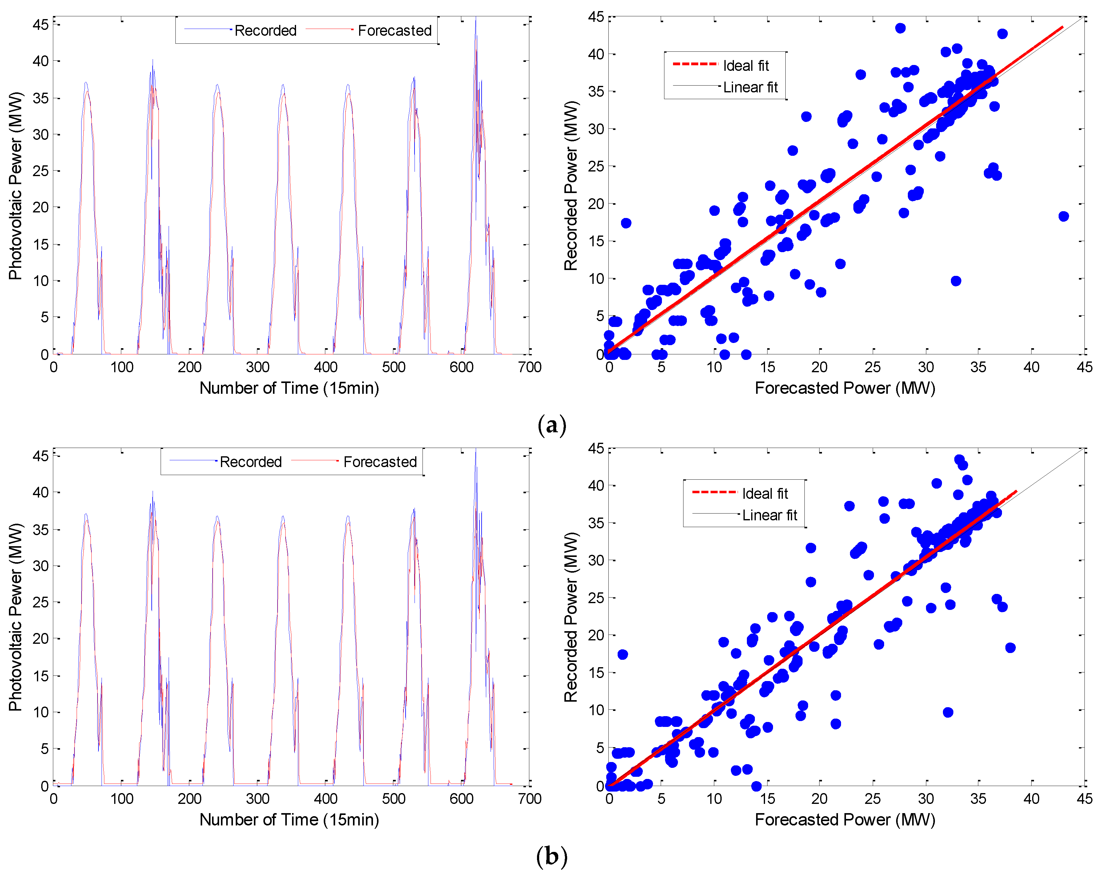
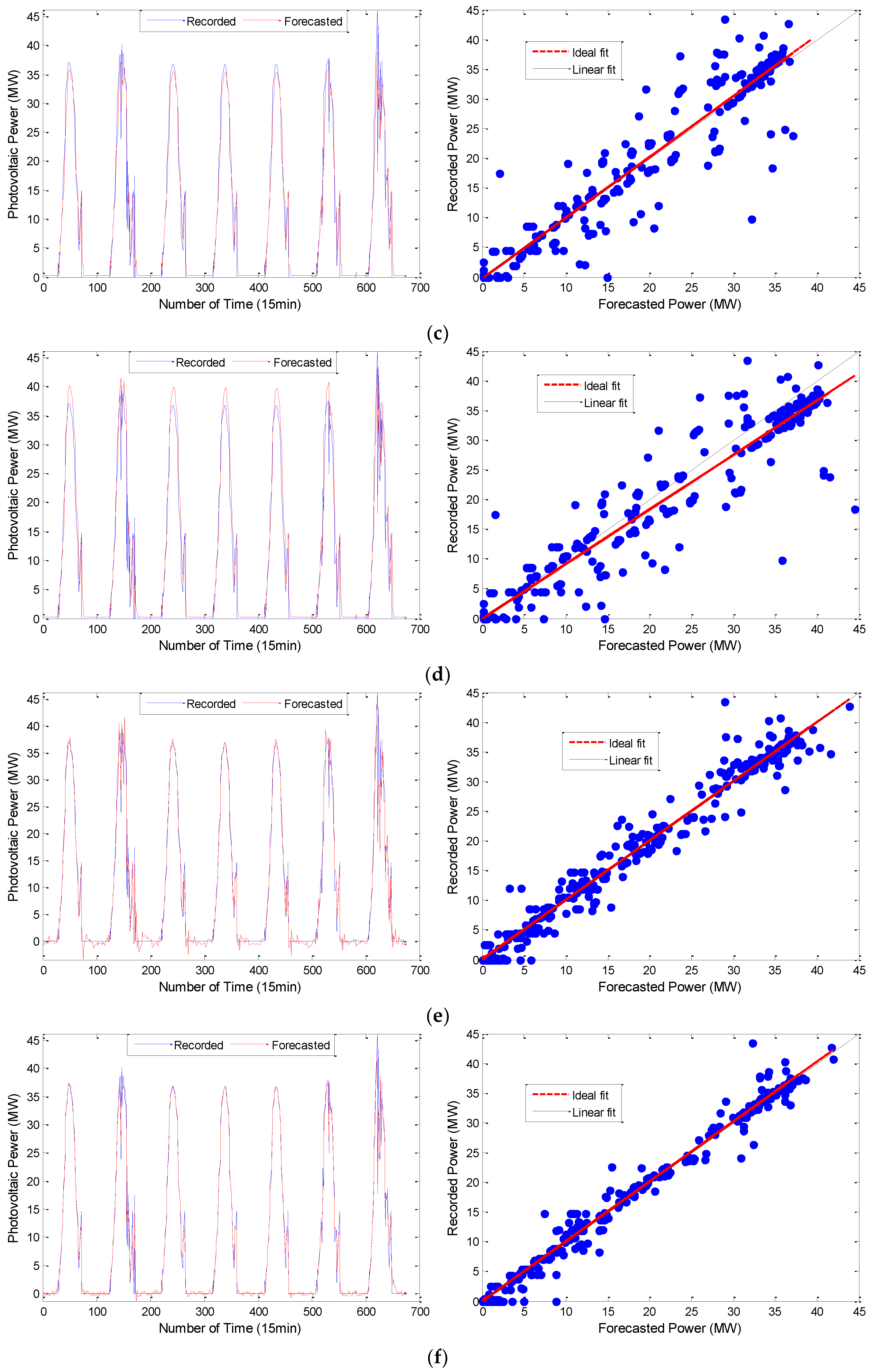
To test the prediction effect of the model proposed in this paper, we compared the results of the following prediction models: (1) the single prediction models (ARMA, DBN) used in this paper; (2) the common neural network prediction model, RNN and Gradient Boost Decision Tree (GBDT) in literature [46,47], used on a representative basis; (3) the combined prediction model, Discrete Wavelet Transformation (DWT) in literature [48] and traditional EMD and EEMD are used on a representative basis. The prediction results for each model are shown in Figure 11.

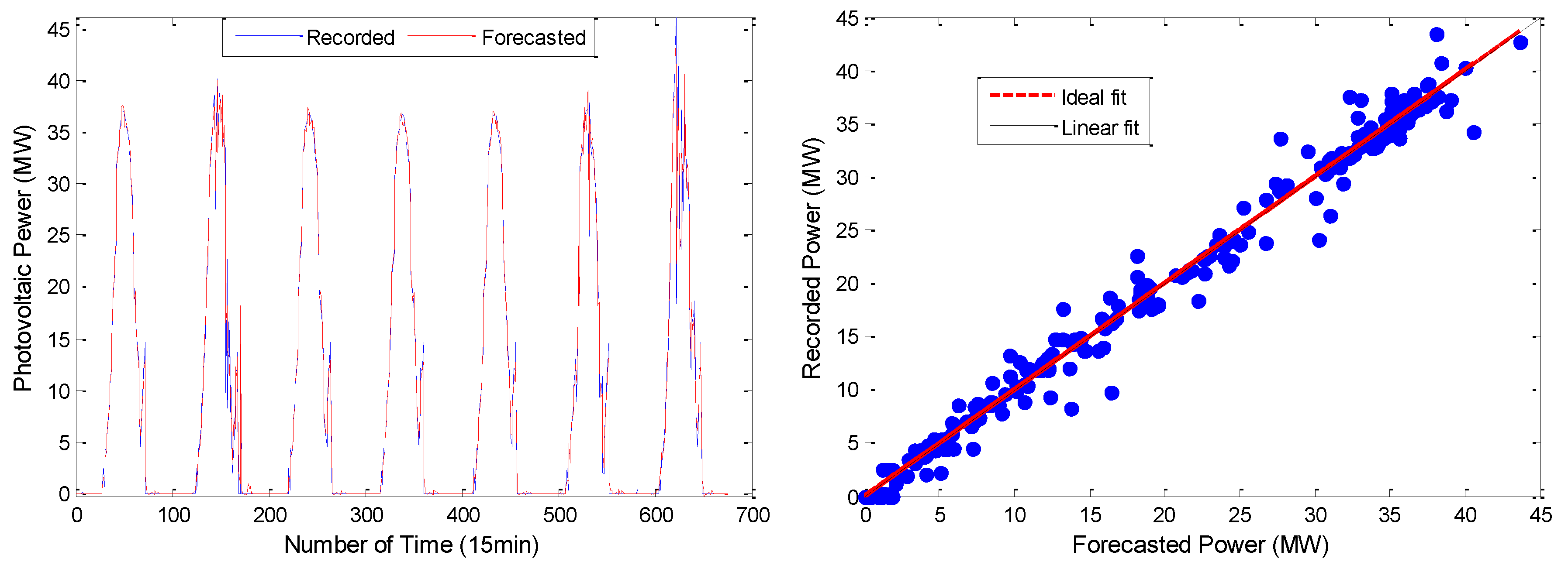
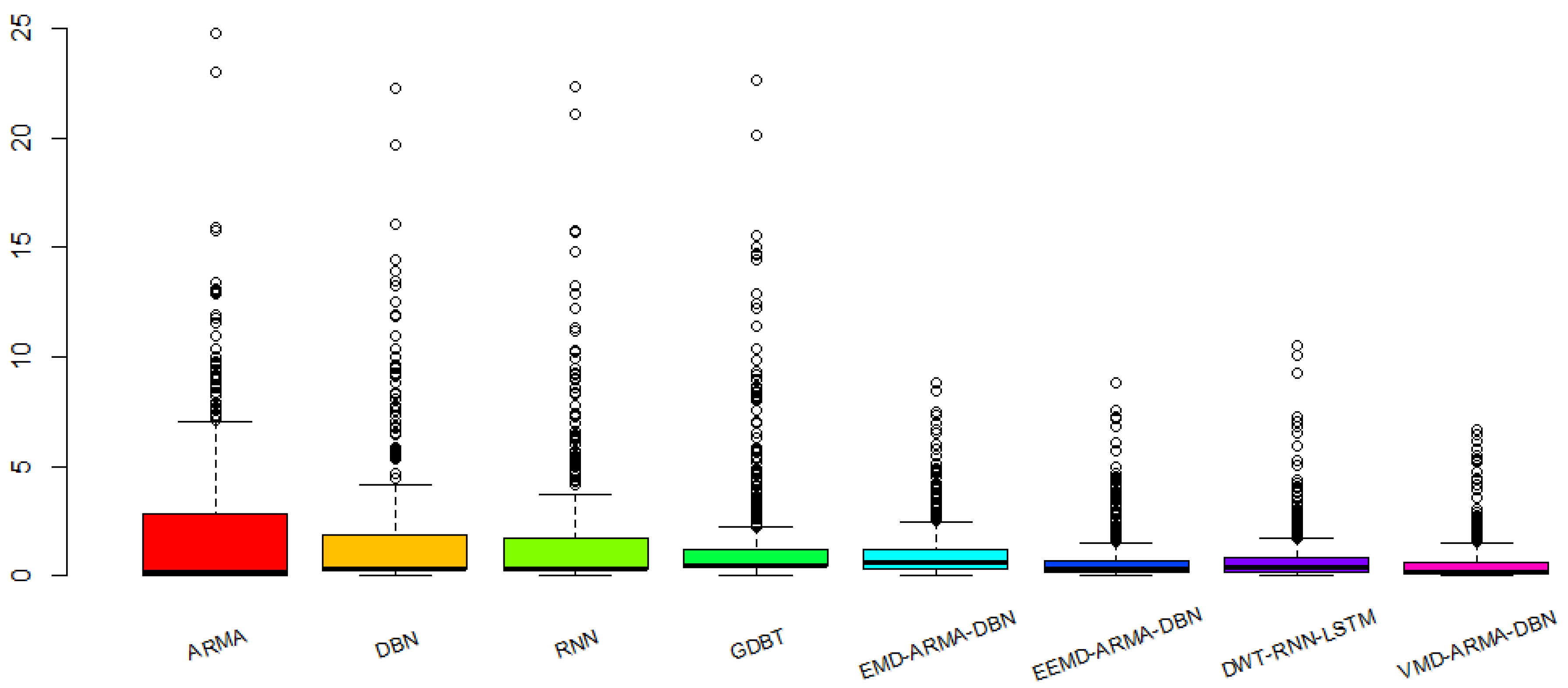
From the simulation results shown in Figure 10 and Figure 11, the VMD-ARMA-DBN combined models have a better tracking and fitting ability for the PV output curve. Compared to the single models, the combined model prediction accuracy (after using the modal decomposition technique) shows different degrees of improvement. Figure 12 is a bar graph demonstrating the absolute error of prediction in each model.

From the perspective of the absolute error distribution of the prediction results, the stability of the prediction accuracy for the single models is poor, and the error distribution interval is large. Among them, the absolute error distribution interval of each model is [0, 24.7821], [0.0051, 22.2464], [0.0082, 22.3289], [0.0363, 22.6686], [0.0005, 8.8306], [0.0018, 8.7955], [0.0008, 10.5322], and [0.0017, 6.6526], respectively, and the prediction error median is 0.1692, 0.2791, 0.2708, 0.4523, 0.5926, 0.3078, 0.0351, and 0.1414, respectively. The absolute error distribution of the VMD-ARMA-DBN model is more concentrated and the median of the error is the smallest, which is the most ideal of the eight groups of prediction models. In summary, the VMD-based multi-frequency combined forecasting model presented in this paper is superior to other models. To compare the prediction effects of each model more intuitively, we used quantitative evaluation indicators.

Table 6. Forecast results for each model.

Evaluation Index	${\mathit{e}}_{\mathit{N}\mathit{M}\mathit{A}\mathit{E}}$	${\mathit{e}}_{\mathit{N}\mathit{R}\mathit{M}\mathit{S}\mathit{E}}$	$\mathit{T}\mathit{I}\mathit{C}$
ARMA	3.74146	7.17435	0.11359
DBN	3.19754	6.43502	0.10139
RNN	3.21145	6.548871	0.10328
GBDT	3.27612	6.434691	0.10812
EMD-ARMA-DBN	2.11062	3.49985	0.05456
EEMD-ARMA-DBN	1.35409	2.67181	0.04171
DWT-RNN-LSTM	1.48241	2.74976	0.04265
VMD-ARMA-DBN	1.03374	2.05776	0.03201

shows the evaluation results for each model.

First, it can be concluded from Figure 12 and Table 6 that, compared with the single prediction models containing ARMA, DBN, RNN, and GBDT, the introduction of the modal decomposition method has a great influence on the accuracy of the prediction results. The modal decomposition method is used to effectively decompose the original PV output, and the prediction method is selected according to the characteristics of different modal vectors, which can make the prediction result more accurate and stable, and the result can be anticipated. The PV system power output has high volatility, variability, and randomness; through modal decomposition it can effectively eliminate the unrelated noise components to make each component easier to predict. In the single prediction models, the error of the ARMA prediction model is the largest, which is not suitable for effectively tracking the undecomposed solar PV output; DBN, RNN and GBDT belong to machine learning, and the prediction error is essentially the same. However, the parameters of the RNN prediction model are more difficult to choose and more easily fall into the local optimum, and GBDT is easy to over-fit for complex models. However, combined prediction methods can effectively avoid these problems.

Second, the proposed VMD-ARMA-DBN model prediction results are always better than those of other combined prediction models (such as EMD, EEMD, and DWT). This is mainly because different decomposition methods have different ways of controlling the modal number, affecting the size of the prediction error. The center frequency of the VMD modal decomposition is controllable, which can effectively avoid modal aliasing compared with other modal decomposition models. The original sequences are decomposed according to the frequency components, and different prediction models are used for fitting purposes. According to the prediction results in Table 6, this kind of combined prediction method significantly improves the prediction accuracy.

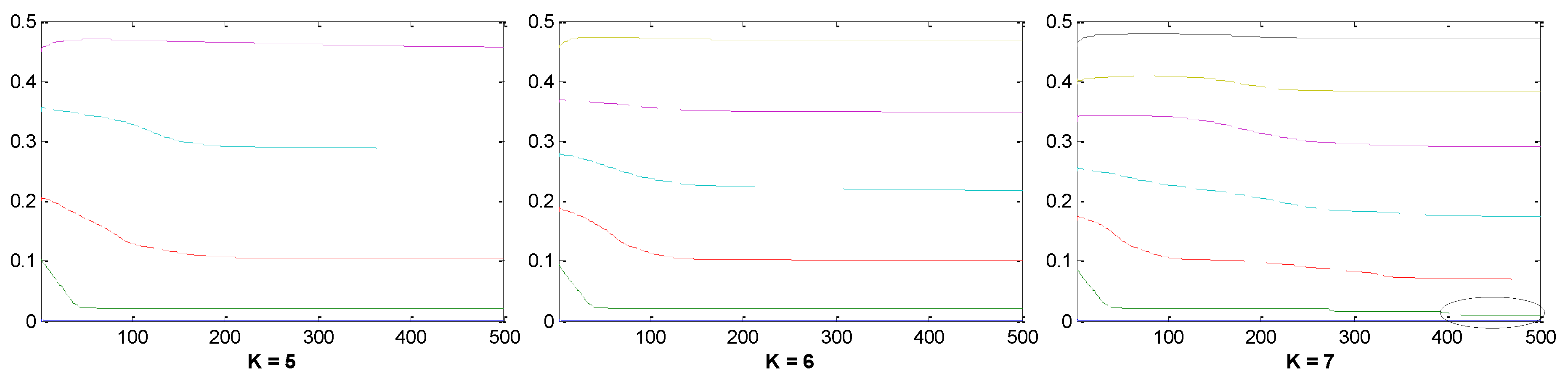
Finally, it should be noted that the prediction results of the VMD-ARMA-DBN models are different under different modal center frequencies K. Specifically, when K is too large, it is easy to cause excessive frequency decomposition, which increases the degree of complexity of the model prediction; when K is too small, it will cause modal overlapping, and the single frequency components cannot be effectively predicted, so only the appropriate K can be used to make an effective prediction. Moreover, this will be an important problem that must be overcome in the next research stage.

5. Conclusions

The short-term prediction accuracy of the nonlinear PV power time series in this work proposes a multi-frequency combined prediction model based on VMD mode decomposition. Specifically, the following was observed:

(1) For the first time, this paper introduces the VMD method into PV power plant output forecasting, decomposes the unstable PV output sequence, and conducts in-depth research on the characteristics of VMD. When traditional decomposition methods deal with sequences that contain both trend and wave terms, accurately extracting the shortcomings of the trend items is impossible. A combination method based on VMD-ARMA-DBN is proposed, which not only reflects the development trend of the size of PV output, but also decomposes the fluctuation series into a set of less complex and some strong periodical parameters, which greatly reduced the difficulty of prediction.

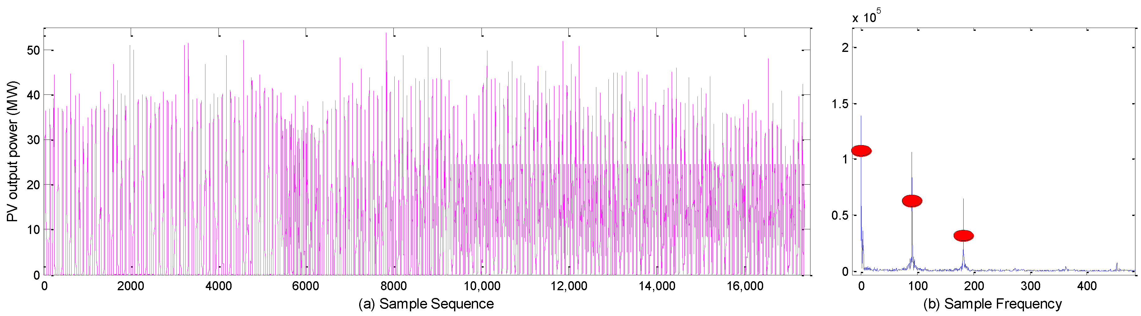
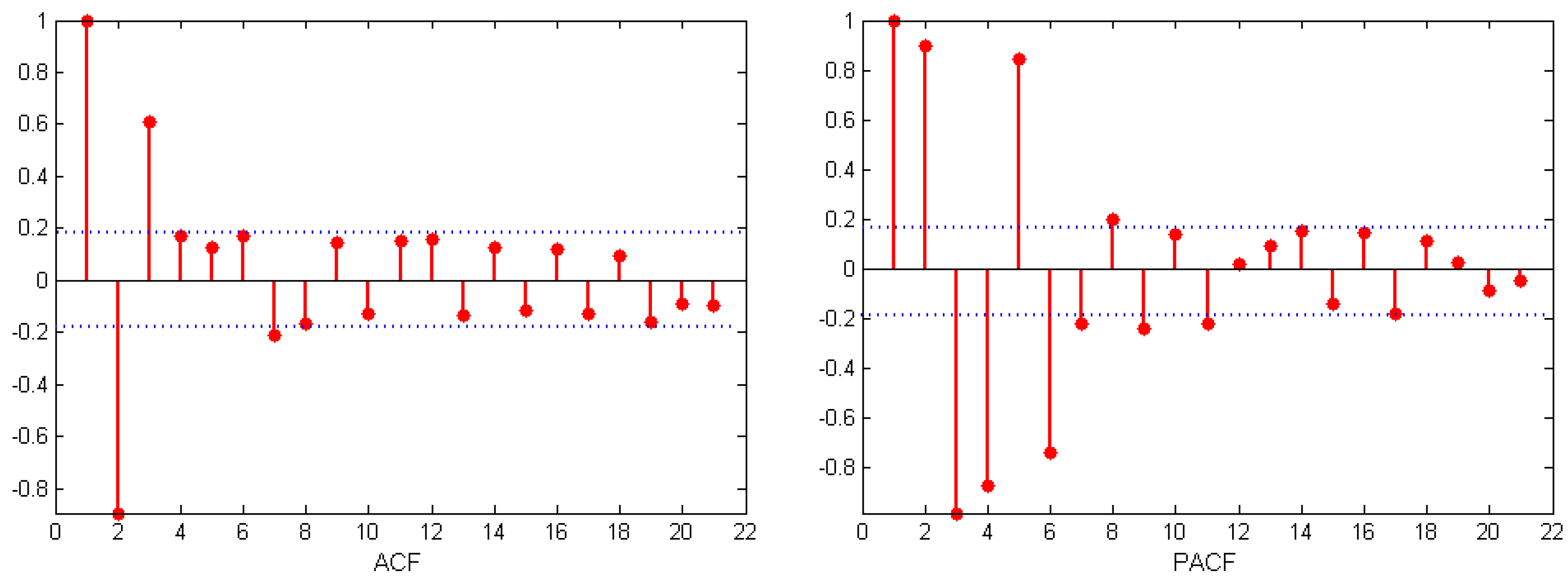
(2) If the VMD cannot restore the original sequence completely, and cannot determine the number of decomposition layers automatically, we propose a method to determine the number of VMD decomposition layers via a spectrum analysis, which can restore the original sequence to a large extent and ensure the stability of the component. First, according to the spectrum diagram of the sample data, we determined the number of modal components. If the overlapping phenomenon occurred in the center frequency iteration curve, the number of decompositions was selected and divided into high- and low-frequency components according to the characteristics of the different components. ARMA and DBN were used to simulate and predict high-frequency and low-frequency components. Then, the predictive value of each component was determined using DBN. Each one had a strong nonlinear mapping ability, and high self-learning ability and self-adaptive capability. The sample data of each component was taken as input, and the actual PV sample value was used as an output to train the model. Then, the predicted value of each component was used as input for the prediction. Finally, the PV output predicted value was obtained.

(3) To test the prediction effect of the VMD combinatorial model, the normalized absolute mean error, normalized root-mean-square error, and the Hill inequality coefficient were used to compare the single prediction models with the combined prediction models. The simulation results show that the different decomposition methods have been improved to varying degrees in terms of forecast accuracy. Thus, the VMD-ARMA-DBN model proposed in this work offers better accuracy and stability than the single prediction methods and the combined prediction models.

In the prediction process, we found that although the VMD improved the phenomenon of modal aliasing and false components, it was not eliminated. In addition, the DBN’s component--RBM needs to be further improved. The weight and offset of each layer of RBM are initialized during training. Therefore, even if the number of hidden layer nodes is compared and selected, the optimal model cannot be obtained, and the final prediction result will show diversification; that is, the same model yields different results, and to obtain optimal results, it is necessary to train the model multiple times, which makes the workload cumbersome. The above deficiencies inevitably increase the errors in the prediction process of each component and affect the final prediction results.

References

1. Gobind, P.; Husain, A. Techno-economic potential of largescale photovoltaics in Bahrain. Sustain. Energy Technol. Assess. 2018, 27, 40–45. [Google Scholar] [CrossRef]
2. Eltawil, M.; Zhao, Z. Grid-connected photovoltaic power systems: Technical and potential problems-a review. Renew. Sustain. Energy Rev. 2010, 14, 112–129. [Google Scholar] [CrossRef]
3. Atsushi, Y.; Tomonobu, S.Y. Determination Method of Insolation Prediction with Fuzzy and Applying Neural Network for Long-Term Ahead PV Power Output Correction. IEEE Trans. Sustain. Energy 2013, 4, 527–533. [Google Scholar] [CrossRef]
4. Shi, J.; Lee, W.J. Forecasting power output of photovoltaic systems based on weather classification and support vector machines. IEEE Trans. Ind. Appl. 2012, 48, 1064–1069. [Google Scholar] [CrossRef]
5. Selmin, E.; Rusen, A. Coupling satellite images with surface measurements of bright sunshine hours to estimate daily solar irradiation on horizontal surface. Renew. Energy 2013, 55, 212–219. [Google Scholar] [CrossRef]
6. Ricardo, M.; Hugo, T.C. Hybrid solar forecasting method uses satellite imaging and ground telemetry as inputs to ANNs. Sol. Energy 2013, 92, 176–188. [Google Scholar] [CrossRef]
7. Wang, J.Z.; Jiang, H. Forecasting solar radiation using an optimized hybrid model by Cuckoo Search algorithm. Energy 2015, 81, 627–644. [Google Scholar] [CrossRef]
8. Bone, V.; Pidgeon, J. Intra-hour direct normal irradiance forecasting through adaptive clear-sky modelling and cloud tracking. Sol. Energy 2018, 159, 852–867. [Google Scholar] [CrossRef]
9. Costa, E.B.; Serra, G.L. Self-Tuning Robust Fuzzy Controller Design Based on Multi-Objective Particle Swarm Optimization Adaptation Mechanism. J. Dyn. Syst. Meas. Control ASME 2017, 139, 071009. [Google Scholar] [CrossRef]
10. Atrsaei, A.; Alarieh, H. Human Arm Motion Tracking by Inertial/Magnetic Sensors Using Unscented Kalman Filter and Relative Motion Constraint. J. Intell. Robot. Syst. 2018, 90, 161–170. [Google Scholar] [CrossRef]
11. Xia, L.; Ma, Z.J. A model-based design optimization strategy for ground source heat pump systems with integrated photovoltaic thermal collectors. Appl. Energy 2018, 214, 178–190. [Google Scholar] [CrossRef]
12. Al-Waeli, A.H.; Sopian, K. Comparison of prediction methods of PV/T nanofluid and nano-PCM system using a measured dataset and artificial neural network. Sol. Energy 2018, 162, 378–396. [Google Scholar] [CrossRef]
13. Yousif, J.H.; Kazem, H.A. Predictive Models for Photovoltaic Electricity Production in Hot Weather Conditions. Energies 2017, 10, 971. [Google Scholar] [CrossRef]
14. Wang, F.; Zhen, Z. Comparative Study on KNN and SVM Based Weather Classification Models for Day Ahead Short Term Solar PV Power Forecasting. Appl. Sci.-Basel 2018, 8, 28. [Google Scholar] [CrossRef]
15. Eseye, A.T.; Zhang, J.H. Short-term photovoltaic solar power forecasting using a hybrid Wavelet-PSO-SVM model based on SCADA and Meteorological information. Renew. Energy 2018, 118, 357–367. [Google Scholar] [CrossRef]
16. Shan, Y.H.; Fu, Q. Combined Forecasting of Photovoltaic Power Generation in Microgrid Based on the Improved BP-SVM-ELM and SOM-LSF With Particlization. Proc. CSEE 2016, 36, 3334–3342. [Google Scholar]
17. Semero, Y.K.; Zheng, D.H. A PSO-ANFIS based Hybrid Approach for Short Term PV Power Prediction in Microgrids. Electr. Power Compon. Syst. 2018, 46, 95–103. [Google Scholar] [CrossRef]
18. Liu, D.; Niu, D.X. Short-term wind speed forecasting using wavelet transform and support vector machines optimized by genetic algorithm. Renew. Energy 2014, 62, 592–597. [Google Scholar] [CrossRef]
19. Farhan, M.A.; Swarup, K.S. Mathematical morphology-based islanding detection for distributed generation. IET Gener. Transm. Dis. 2017, 11, 3449–3457. [Google Scholar] [CrossRef]
20. Liu, H.; Chen, C. A hybrid model for wind speed prediction using empirical mode decomposition and artificial neural networks. Renew. Energy 2012, 48, 545–556. [Google Scholar] [CrossRef]
21. Dai, S.Y.; Niu, D.X. Daily Peak Load Forecasting Based on Complete Ensemble Empirical Mode Decomposition with Adaptive Noise and Support Vector Machine Optimized by Modified Grey Wolf Optimization Algorithm. Energies 2018, 11, 163. [Google Scholar] [CrossRef]
22. Sun, B.; Yao, H. Short-term wind speed forecasting based on local mean decomposition and multi-kernel support vector machine. Acta Energiae Solaris Sin. 2013, 34, 1567–1573. [Google Scholar]
23. Zhu, T.; Wei, H. Clear-sky model for wavelet forecast of direct normal irradiance. Renew. Energy 2017, 104, 1–8. [Google Scholar] [CrossRef]
24. Li, F.; Wang, S. Long term rolling prediction model for solar radiation combining empirical mode decomposition (EMD) and artificial neural network (ANN) techniques. J. Renew. Sustain. Energy 2018, 10, 013704. [Google Scholar] [CrossRef]
25. Wang, L.; Liu, Z.W. Complete ensemble local mean decomposition with adaptive noise and its application to fault diagnosis for rolling bearings. Mech. Syst. Signal Process. 2018, 106, 24–39. [Google Scholar] [CrossRef]
26. Wang, C.; Zhang, H.L. A new chaotic time series hybrid prediction method of wind power based on EEMD-SE and full-parameters continued fraction. Energy 2017, 138, 977–990. [Google Scholar] [CrossRef]
27. Zhang, Y.C.; Liu, K.P. Short-Term Wind Power Multi-Leveled Combined Forecasting Model Based on Variational Mode Decomposition-Sample Entropy and Machine Learning Algorithms. Power Syst. Technol. 2016, 40, 1334–1340. [Google Scholar] [CrossRef]
28. Liu, C.L.; Wu, Y.J. Rolling bearing fault diagnosis based on variational model decomposition and fuzzy C means clustering. Proc. CSEE 2015, 35, 3358–3365. [Google Scholar]
29. Dragomiretskiy, K.; Zosso, D. Variational mode decomposition. IEEE Trans. Signal Process. 2014, 62, 531–544. [Google Scholar] [CrossRef]
30. Naik, J.; Dash, S. Short term wind power forecasting using hybrid variational mode decomposition and multi-kernel regularized pseudo inverse neural network. Renew. Energy 2018, 118, 180–212. [Google Scholar] [CrossRef]
31. Li, C.S.; Xiao, Z.G. A hybrid model based on synchronous optimisation for multi-step short-term wind speed forecasting. Appl. Energy 2018, 215, 131–144. [Google Scholar] [CrossRef]
32. Hinton, G.; Salakhutdinov, R. Reducing the dimensionality of data with neural networks. Science 2006, 313, 504–507. [Google Scholar] [CrossRef] [PubMed]
33. Zhu, Q.M.; Dang, J. A Method for Power System Transient Stability Assessment Based on Deep Belief Networks. Proc. CSEE 2018, 38, 735–743. [Google Scholar]
34. Hinton, G.; Deng, L. Deep neural networks for acoustic modeling in speech recognition: The shared views of four research groups. IEEE Signal Process. Mag. 2012, 29, 82–97. [Google Scholar] [CrossRef]
35. Hinton, G. Training products of experts by minimizing contrastive divergence. Neural Comput. 2002, 14, 1771–1800. [Google Scholar] [CrossRef] [PubMed]
36. Wang, Y.J.; Na, X.D. State Recognition Method of a Rolling Bearing Based on EEMD-Hilbert Envelope Spectrum and DBN Under Variable Load. Proc. CSEE 2017, 37, 6943–6950. [Google Scholar]
37. Tian, B.; Piao, Z.L. Wind power ultra short-term model based on improved EEMD-SE-ARMA. Power Syst. Protect. Control 2017, 45, 72–79. [Google Scholar]
38. Yang, Z.; Ce, L. Electricity price forecasting by a hybrid model, combining wavelet transform, ARMA and kernel-based extreme learning machine methods. Appl. Energy 2017, 190, 291–305. [Google Scholar] [CrossRef]
39. Li, C.B.; Zheng, X.S. Predicting Short-Term Electricity Demand by Combining the Advantages of ARMA and XG Boost in Fog Computing Environment. Wirel. Commun. Mob. Comput. 2018, 5018053. [Google Scholar] [CrossRef]
40. Lu, J.L.; Wang, B. Two-Tier Reactive Power and Voltage Control Strategy Based on ARMA Renewable Power Forecasting Models. Energies 2017, 10, 1518. [Google Scholar] [CrossRef]
41. Li, L.; Zhang, S.F. Ionospheric total electron content prediction based on ARMA model. J. Basic Sci. Eng. 2013, 21, 814–822. [Google Scholar]
42. Wu, J.; Chan, C.K. Prediction of hourly solar radiation using a novel hybrid model of ARMA and TDN. Sol. Energy 2011, 85, 808–817. [Google Scholar] [CrossRef]
43. Voyant, C.; Muselli, M. Numerical weather prediction (NWP) and hybrid ARMA/ANN model to predict global radiation. Energy 2012, 39, 341–355. [Google Scholar] [CrossRef] [Green Version]
44. Alshamaa, D.; Chehade, F.M. A hierarchical classification method using belief functions. Signal Process. 2018, 148, 68–77. [Google Scholar] [CrossRef]
45. Fu, G.Y. Deep belief network based ensemble approach for cooling load forecasting of air-conditioning system. Energy 2018, 148, 269–282. [Google Scholar] [CrossRef]
46. Zhang, B.; Wu, J.L.; Chang, P.C. A multiple time series-based recurrent neural network for short-term load forecasting. Soft Comput. 2018, 22, 4099–4112. [Google Scholar] [CrossRef]
47. Wang, F.; Yu, Y.L.; Zhang, Z.Y. Wavelet Decomposition and Convolutional LSTM Networks Based Improved Deep Learning Model for Solar Irradiance Forecasting. Appl. Sci.-Basel 2018, 8, 1286. [Google Scholar] [CrossRef]
48. Wang, J.D.; Li, P.; Ran, R. A Short-Term Photovoltaic Power Prediction Model Based on the Gradient Boost Decision Tree. Appl. Sci.-Basel 2018, 8, 689. [Google Scholar] [CrossRef]
Figure 1. Deep belief network structure. RBM: Restricted Boltzmann Machine; BP: Back-Projection.
Applsci 08 01901 g001
Figure 2. RBM structure diagram (V stands for the display element and h stands for the hidden element).
Applsci 08 01901 g002
Figure 3. Combination Forecasting Model Based on VMD-ARMA-DBN. PV: photovoltaic; IMF: Intrinsic Mode Function; VMD: Variational Mode Decomposition; DBN: Deep Belief Network.
Applsci 08 01901 g003
Figure 4. Photovoltaic output sample sequence.
Applsci 08 01901 g004
Figure 5. Sample center frequency iteration curves in different modes.
Applsci 08 01901 g005
Figure 6. VMD decomposition diagram and spectrum diagram. (a) Modal components, (b) Frequency.
Applsci 08 01901 g006
Figure 7. Prediction of IMF1-IMF3 component.
Applsci 08 01901 g007
Figure 8. The autocorrelation function (ACF) and partial autocorrelation function (PACF) of IMF4 decomposed.
Applsci 08 01901 g008
Figure 9. IMF4-IMF6 component prediction.
Applsci 08 01901 g009
Figure 10. VMD-ARMA-DBN combination forecast results.
Applsci 08 01901 g010
Figure 11. Prediction results for multiple models. (a) ARMA model prediction results; (b) DBN model prediction results; (c) RNN model prediction results; (d) GBDT model prediction results; (e) EMD-ARMA-DBN model prediction results; (f) EEMD-ARMA-DBN model prediction results; (g) DWT-RNN-LSTM model prediction results. RNN: Recurrent Neural Network; GBDT: Gradient Boost Decision Tree; EEMD: Ensemble Empirical Mode Decomposition; DWT: Discrete Wavelet Transformation; LSTM: Long Short-Term Memory.
Applsci 08 01901 g011aApplsci 08 01901 g011bApplsci 08 01901 g011c
Figure 12. Simulation results of each model: absolute error box plot.
Applsci 08 01901 g012