LPV Model Based Sensor Fault Diagnosis and Isolation for Permanent Magnet Synchronous Generator in Wind Energy Conversion Systems

Abstract

This paper deals with the current sensor fault diagnosis and isolation (FDI) problem for a permanent magnet synchronous generator (PMSG) based wind system. An observer based scheme is presented to detect and isolate both additive and multiplicative faults in current sensors, under varying torque and speed. This scheme includes a robust residual generator and a fault estimation based isolator. First, the PMSG system model is reformulated as a linear parameter varying (LPV) model by incorporating the electromechanical dynamics into the current dynamics. Then, polytopic decomposition is introduced for ${\mathcal{H}}_{\infty }$ design of an LPV residual generator and fault estimator in the form of linear matrix inequalities (LMIs). The proposed gain-scheduled FDI is capable of online monitoring three-phase currents and isolating multiple sensor faults by comparing the diagnosis variables with the predefined thresholds. Finally, a MATLAB/SIMULINK model of wind conversion system is established to illustrate FDI performance of the proposed method. The results show that multiple sensor faults are isolated simultaneously with varying input torque and mechanical power.

1. Introduction

Due to the high power density and efficiency, permanent magnet synchronous generator based wind turbines are promising in wind conversion systems (WECSs) with variable speed operation and full-scale power delivery [1,2]. To fulfill control demands for maximum power point tracking (MPPT) and grid codes, closed-loop feedback control is designed, relying on the mechanical, current and voltage measurements. Any inaccurate measurements caused by sensor faults will cause the controller malfunction and performance degradation. According to industrial and field statistics [3,4,5], current sensor faults are a type of major faults resulting from the electromagnetic interference and high power density, which causes system shutdown and fragile components.

Fault diagnosis and isolation (FDI) schemes enable the control system to locate fault sensors and to compensate the fault further. For power converter systems, various diagnostic techniques are presented to handle current sensor FDI problems, including observer based, signal processing based and data-driven based methods. Model based diagnostic techniques are discussed most for power converter systems. A parallel observers based method is presented in [6] to diagnose stator and rotor current sensor faults in doubly fed induction generator (DFIG) system, but it requires open-loop operation while detecting the sensor fault. Similarly, a sensor FDI in [7] that a bank of observers are designed to generate residuals sensitive to sensor fault for DFIG based WECSs also requires open-loop operation until the fault is isolated. In [8], a geometric approach is presented to detect and isolate multiple sensor faults in induction motor (IM) drives. By utilizing the redundant properties of three-phase currents, two stationary frame based state space models are established to generate distinguished residuals sensitive to phase a and phase b sensor faults. In [9], the nonlinear model of DFIG is transformed into a Takagi–Sugeno (T-S) fuzzy model and a bank of observers based on the model are presented to generate residuals for sensor fault detection and isolation. To deal with both additive and multiplicative sensor faults, a generalized observer scheme is presented in [10] by combining $\mathcal{H}\_/{\mathcal{H}}_{\infty }$ filter with Kalman-like observer for DFIG systems.

Aforementioned schemes are presented for sensor FDI in IM drives while only a few model based sensor FDIs are proposed for permanent magnet synchronous motor (PMSM) and permanent magnet synchronous generator (PMSG) systems. In [11], a two-stage extended Kalman filter (EKF) and adaptive observer is presented to generate mechanical estimations for speed and rotor position sensor fault diagnosis. An adaptive EKF for position sensor fault diagnosis and tolerant scheme is presented in [12] for PMSM drive in electric vehicle (EV). In [13], a high-order sliding model based observer is proposed to detect and estimate rotor speed sensor fault in PMSM based EV. The authors later present a bank of observers based scheme for multiple sensor FDI [14]. However, it requires additional voltage sensors to establish the fault observers. In [15], an EKF based FDI is presented for the diagnosis of sensor fault in PMSM drives, but it can only isolate single sensor faults and does not additionally discuss about the influence of unknown disturbances on FDI performance. Furthermore, in [2], to diagnose additive and multiplicative faults for PMSG based WECSs, a two-stage model based method is proposed, in which time-varying Kalman filter (TVKF) and maximum-shift method are designed to generate robust residuals and evaluate these residuals.

According to the state-of-the-art analysis, model based FDI methods are rarely reported for simultaneous multiple current sensor FDI for PMSM and PMSG based applications. Nevertheless, current sensor FDI is necessary for control system in power converters to provide further information for fault tolerant control [2,8]. In this paper, an observer based scheme is presented to detect and isolate both additive and multiplicative faults in current sensors under varying torque and speed. The proposed method includes a robust residual generator and a fault estimation based isolator. The system model is established in the stationary reference frame and the nonlinear term with rotor position is transformed into a polytopic linear parameter varying (LPV) model. Based on the stability and convergency analysis, a gain-scheduled fault detector and isolator is designed in the form linear matrix inequalities (LMIs). The proposed gain-scheduled FDI scheme is capable of online monitoring three-phase currents and isolating multiple sensor faults with only one fault estimator. Comparing with the existing methods for current sensor isolation, this method does not require complex observer combination or a bank of observers and can isolate both additive and multiplicative faults. The contributions of this paper are concluded as follows:

(1)

A scheme is proposed for detection and isolation of multiple sensor faults. Compared with the existing methods, the proposed method is capable of isolating three-phase current sensor faults while most existing schemes are presented to isolate faults in stationary frame or synchronous reference frame.

(2)

The proposed isolator is based on a fault estimation scheme. Fault estimates contain all the fault information, which makes it possible to deal with both additive and multiplicative faults.

(3)

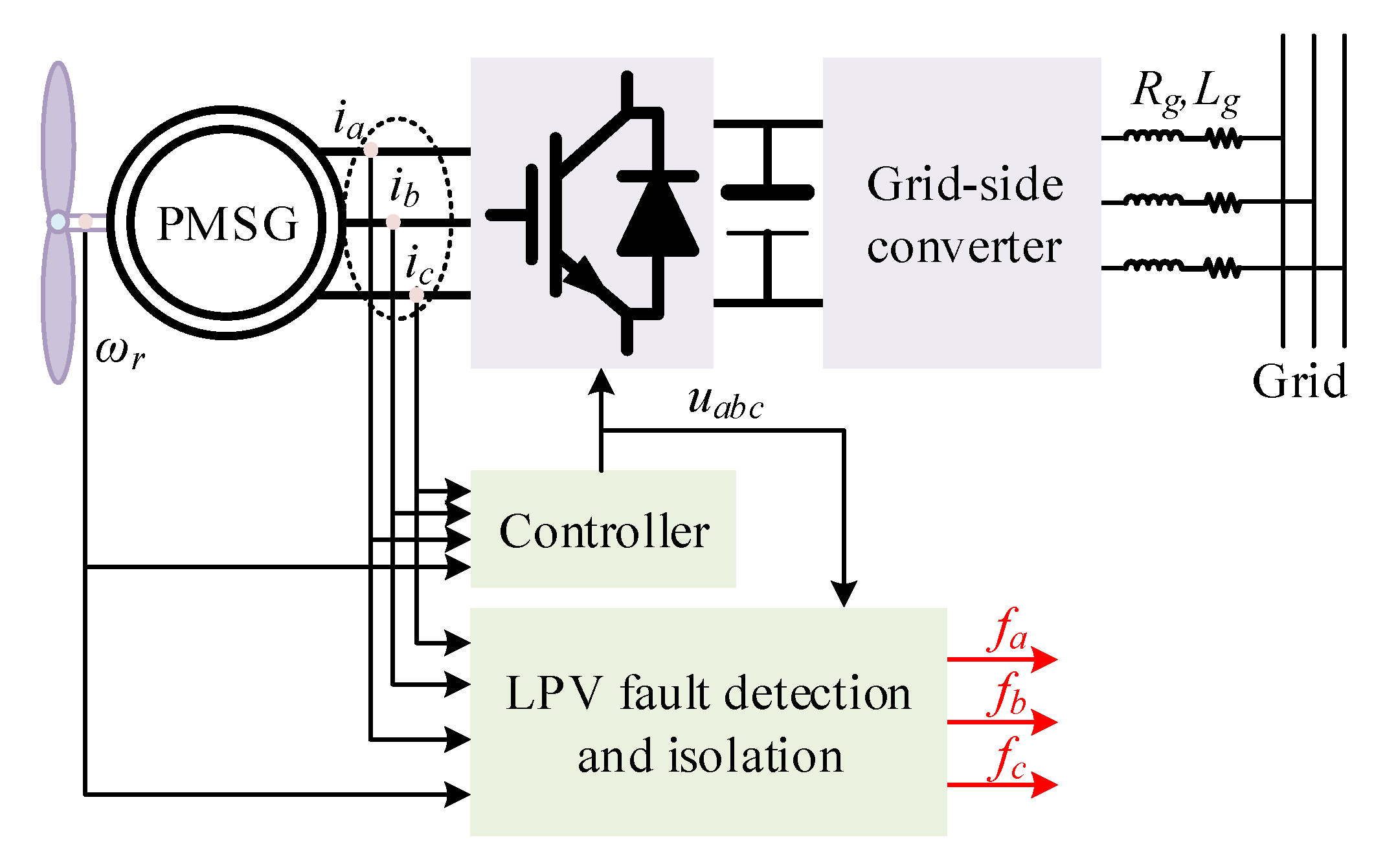
All of the measurements are available in the control loop. No additional hardware or measurements are required. Furthermore, the proposed method is implemented in closed-loop operation.

The rest of this paper is organized as follows. Section 2 establishes PMSG and sensor fault model, and polytopic decomposition of the model. The gain-scheduled observer design for fault detection residuals generation is presented in Section 3. In Section 4, a fault estimation design scheme is presented for isolation of each phase current sensor fault. The simulation results are presented in Section 5 to illustrate the performance of proposed method. Finally, the conclusion is presented in Section 6.

2. Problem Statement

The system configuration of PMSG based WECS is shown in Figure 1. Typically, a full-scale back-to-back converter is designed as the interface between generator and the electrical grid. The field-oriented control (FOC) is employed to transfer maximum power generated by wind turbine while tracking the rotor speed reference that requires measured values of rotor position $\theta$, rotor speed ${\omega }_r$ and three-phase currents $i_a$, $i_b$, $i_c$.

Machine-side control is designed to implement an MPPT scheme for variable-speed WECSs. Each wind turbine operates in a certain wind speed region according to its ideal power curve. This leads a varying rotor speed or torque to feed the generator. As shown in Figure 2, generator stops in Regions I and IV while it continues to generate electrical power in Regions II and III.

The mechanical signals and current measurements are crucial to ensure a stable and optimal operating condition of the WECSs. Any sensor malfunction will be fed back into the control system, which could cause performance reduction or even system downtime. Sensor faults are investigated in [11] and exhibited as: (1) sensor gain drop Type a; (2) bias in sensor measurement Type b and (3) complete sensor outage Type c. Type b and Type a faults can be modeled as an addictive fault in sensor measurements

$$y_m\left(k\right)=y_r\left(k\right)+f\left(k\right)$$

(1)

in which $y_m\left(k\right)$, $y_r\left(k\right)$ and $f\left(k\right)$ denote the faulty measurements, nominal values and fault signals respectively. Type a fault is the sensor gain degradation and modeled as a multiplicative fault in [2]

$$y_m\left(k\right)=\beta \left(k\right)y_r\left(k\right).$$

(2)

By defining $f\left(k\right)=\left(\beta \left(k\right)-1\right)y_r\left(k\right)$, Type a fault in Equation (2) is rewritten as an additive fault with Formula (1). These three types of faults are uniformly modeled as additive faults.

Remark 1.

In (1), $f\left(k\right)$ is unknown when $k{T}_s>t_{fault}$ ($\forall k{T}_s<t_{fault},f\left(k\right)=0$). A practical assumption of the sensor faults $f\left(k\right)$ is introduced in this paper: $f\left(k\right)$ is ${\mathcal{L}}_2-$ bounded $\parallel f\left(k\right)\parallel \le \parallel \alpha \left(k\right)\parallel$ and $\alpha \left(k\right)$ is a known function. The upper bound of fault is essential for fault estimator design in Theorem 2.

2.1. LPV Model of PMSG

The mathematical model of a surface-mounted PMSG can be expressed in the stationary reference frame as [14,18,19]

$$\begin{array}{cc}\hfill \frac{d{i}_{\alpha }}{dt}& =-\frac{R_s}{L_s}{i}_{\alpha }+\frac{n_p\psi }{L_s}sin\left(\theta \right){\omega }_r+\frac{1}{L_s}{u}_{\alpha }\hfill \\ \hfill \frac{d{i}_{\beta }}{dt}& =-\frac{R_s}{L_s}{i}_{\beta }-\frac{n_p\psi }{L_s}cos\left(\theta \right){\omega }_r+\frac{1}{L_s}{u}_{\beta }\hfill \\ \hfill \frac{d{\omega }_r}{dt}& =-\frac{3n_p\psi }{2J}sin\left(\theta \right)i_{\alpha }+\frac{3n_p\psi }{2J}cos\left(\theta \right)i_{\beta }-\frac{F}{J}{\omega }_r-\frac{1}{J}{T}_L\hfill \\ \hfill \frac{d\theta }{dt}& =n_p{\omega }_r,\hfill \end{array}$$

(3)

where $i_{\alpha }$, $i_{\beta }$ and $u_{\alpha }$, $u_{\beta }$ are the currents [A] and voltages [V] of phases $\alpha$ and $\beta$ in the stationary frame, respectively. In addition, $\theta$ is rotor electrical angle [rad]; ${\omega }_r$ denotes rotor velocity [rad/s]; F is the viscous friction coefficient [N·m·s/rad]; $T_L$ is the load torque [N·m]; J is the inertia of the motor [Kg·m${}^2$]; $\psi$ is the magnetic flux of the motor [Wb]; $R_s$ is the resistances of the phase winding [$\Omega$]; L is the inductance of the phase winding [H]; $n_p$ is the number of pairs of rotor poles.

By defining state variables $x={\left[i_{\alpha },i_{\beta },{\omega }_r,\theta \right]}^T$ and measurements $y={\left[i_a,i_b,i_c,{\omega }_r,\theta \right]}^T$, system (3) is expressed as a linear parameter varying model

$$\begin{array}{cc}\hfill \dot{x}& =A\left(\theta \right)x+B_{u}u+B_{d}d,\hfill \\ \hfill y& =Cx,\hfill \end{array}$$

(4)

in which $i_a$, $i_b$ and $i_c$ denote three-phase currents of PMSG which are acquired by current sensors. Provided that the currents and voltages remain nearly constant at each sample time interval $T_s$. The Forward Euler Approximation method is introduced for discretization of a PMSG model

$$x\left(k{T}_s+T_s\right)=x\left(k{T}_s\right)+T_s{\left\{\frac{dx\left(t\right)}{dt}\right\}}_{t=k{T}_s},$$

(5)

where $T_s$ is the sampling time. Accordingly, system (4) leads to the following discrete system model:

$$\begin{array}{cc}\hfill x\left(k+1\right)& =A\left({\theta }_k\right)x\left(k\right)+B_{u}u\left(k\right)+B_{d}d\left(k\right),\hfill \\ \hfill y\left(k\right)& =Cx\left(k\right),\hfill \end{array}$$

(6)

where $A\left({\theta }_k\right)$, $B_u$, $B_d$ and C are listed as Equation (A1) in Appendix A.

2.2. Polytopic Decomposition of the System Model

An LPV model of PMSG with sensor faults is presented as follows with bounded varying parameters:

$$\begin{array}{cc}\hfill x\left(k+1\right)& =A\left({\theta }_k\right)x\left(k\right)+B_{u}u\left(k\right)+B_{d}d\left(k\right),\hfill \\ \hfill y\left(k\right)& =Cx\left(k\right)+F_{f}f\left(k\right),\hfill \end{array}$$

(7)

where $F_f$ is the fault distribution matrix. $A\left({\theta }_k\right)$ contains two time-varying terms $sin\left({\theta }_k\right)$ and $cos\left({\theta }_k\right)$, an auxiliary variable is defined $\mu \left({\theta }_k\right)={\left[\begin{array}{cc}{\mu }_1\left({\theta }_k\right)& {\mu }_2\left({\theta }_k\right)\end{array}\right]}^T,$

$$\begin{array}{cc}\hfill {\mu }_1\left({\theta }_k\right)& =sin\left({\theta }_k\right),\hfill \\ \hfill {\mu }_2\left({\theta }_k\right)& =cos\left({\theta }_k\right).\hfill \end{array}$$

(8)

It is obvious that $A\left({\theta }_k\right)$ depends affinely on the parameter $\mu \left({\theta }_k\right)$

$$A\left({\theta }_k\right)={\mathcal{A}}_0+{\mu }_1\left({\theta }_k\right){\mathcal{A}}_1+{\mu }_2\left({\theta }_k\right){\mathcal{A}}_2,$$

(9)

where ${\mathcal{A}}_0$, ${\mathcal{A}}_1$ and ${\mathcal{A}}_2$ are constant matrices. The time-varying parameter vector $\mu \left({\theta }_k\right)$ is determined by the rotor electrical angle ${\theta }_k$. Moreover, ${\mu }_1\left({\theta }_k\right)$ and ${\mu }_2\left({\theta }_k\right)$ are trigonometric function and bounded by the lower and upper bounds

$$\begin{array}{c}{\mu }_1\in \left[\begin{array}{cc}{\underline{\mu }}_1& {\overline{\mu }}_1\end{array}\right]\hfill \\ {\mu }_2\in \left[\begin{array}{cc}{\underline{\mu }}_2& {\overline{\mu }}_2\end{array}\right]\hfill \\ \mu {\left({\theta }_k\right)}^T\mu \left({\theta }_k\right)=1\hfill \end{array}$$

(10)

in which ${\underline{\mu }}_1={\underline{\mu }}_2=-1$ and ${\overline{\mu }}_1={\overline{\mu }}_2=1$. A convex polytope $\Theta$ with four vertices ${\mu }_{v,1}$, ${\mu }_{v,2}$, ${\mu }_{v,3}$, ${\mu }_{v,4}$ is defined to ensure that the trajectory of parameter $\mu \left({\theta }_k\right)$ is enclosed:

$$\begin{array}{cccc}\hfill {\mu }_{v,1}& =\left[\begin{array}{c}{\underline{\mu }}_1\\ {\underline{\mu }}_2\end{array}\right]\hfill & \hfill {\mu }_{v,2}& =\left[\begin{array}{c}{\underline{\mu }}_1\\ {\overline{\mu }}_2\end{array}\right]\hfill \\ \hfill {\mu }_{v,3}& =\left[\begin{array}{c}{\overline{\mu }}_1\\ {\underline{\mu }}_2\end{array}\right]\hfill & \hfill {\mu }_{v,1}& =\left[\begin{array}{c}{\overline{\mu }}_1\\ {\overline{\mu }}_2\end{array}\right].\hfill \end{array}$$

(11)

Consequently, parameter $\mu \left({\theta }_k\right)$ can be expressed as a convex combination of the vertices with coordinates ${\eta }_k={\left[\begin{array}{cccc}{\eta }_{k,1}& {\eta }_{k,2}& {\eta }_{k,3}& {\eta }_{k,4}\end{array}\right]}^T,$

$$\begin{array}{c}\mu \left({\theta }_k\right)=\left[\begin{array}{cccc}{\mu }_{v,1}& {\mu }_{v,2}& {\mu }_{v,3}& {\mu }_{v,4}\end{array}\right]{\eta }_k,\hfill \\ {\eta }_{k,1}+{\eta }_{k,2}+{\eta }_{k,3}+{\eta }_{k,4}=1,\hfill \end{array}$$

(12)

in which $\forall i=1,\cdots ,4$, ${\eta }_{k,i}\ge 0$ and the parameter-dependent matrix $A\left(\mu \right)$ is rewritten by a combination of coordinate vector ${\eta }_k$

$$A\left(\mu \right)=\sum _{i=1}^4{\eta }_{k,i}{A}_{v,i},$$

(13)

in which $A_{v,i}=A\left({\mu }_{v,i}\right)$ with $i=1,\cdots ,4$. The system Equation (7) can be transformed into a polytopic form

$$\begin{array}{cc}\hfill x\left(k+1\right)& =\sum _{i=1}^4{\eta }_{k,i}{A}_{v,i}x\left(k\right)+B_{u}u\left(k\right)+B_{d}d\left(k\right),\hfill \\ \hfill y\left(k\right)& =Cx\left(k\right)+F_{f}f\left(k\right).\hfill \end{array}$$

(14)

Since Equation (12) is an underdetermined equation, further constraints are required to solve this equation. In [20,21,22], a vertex expansion technique is presented to get a unique solution of ${\eta }_k$. Furthermore, this work decomposes $A\left({\theta }_k\right)$ with this method.

2.3. Extended Bounded Real Lemma

This section extends the bounded real lemma to polytopic-LPV system, consider the following systems

$$G_{y\omega }\left(z,\rho \right):\left\{\begin{array}{cc}\hfill x\left(k+1\right)& =A\left(\rho \right)x\left(k\right)+B\left(\rho \right)\omega \left(k\right),\hfill \\ \hfill y\left(k\right)& =C\left(\rho \right)x\left(k\right)+D\left(\rho \right)\omega \left(k\right),\hfill \end{array}\right.$$

(15)

where $x\left(k\right),\omega \left(k\right),y\left(k\right)$ denote the state variables, disturbances and measurements, respectively. $\rho \in {\mathcal{P}}_{\rho }$ is a time-varying parameter vector with ${\rho }_i\in \left[{\underline{\rho }}_i,{\overline{\rho }}_i\right]$. Assuming that parameter space ${\mathcal{P}}_{\rho }$ is a convex hull, the system (15) can be presented as a polytopic form

$$\left[\begin{array}{cc}A\left(\rho \right)& B\left(\rho \right)\\ C\left(\rho \right)& D\left(\rho \right)\end{array}\right]\stackrel{\Delta }{=}\sum _{i=1}^N{\eta }_i\left[\begin{array}{cc}{A}_i& B_i\\ C_i& D_i\end{array}\right],$$

(16)

where N is the number of vertices, ${\displaystyle \sum _{i=1}^N}{\eta }_i=1$ and ${\eta }_i\ge 0$. The ${\mathcal{H}}_{\infty }$ performance is defined as Equation (17) to guarantee the asymptotically stability of system (15)

$$\parallel G_{y\omega }\left(z,\rho \right){\parallel }_{\infty }=\underset{\parallel \omega \left(k\right){\parallel }_2\ne 0}{sup}\frac{\parallel y\left(k\right){\parallel }_2}{\parallel \omega \left(k\right){\parallel }_2}.$$

(17)

An extended Bounded real lemma can be derived from the results in [23,24].

Lemma 1.

Given the system (15) and for all $\rho \in {\mathcal{P}}_{\rho }$, $G_{y\omega }\left(z,\rho \right)$ is asymptotically stable with $\parallel G_{y\omega }\left(z,\rho \right){\parallel }_{\infty }<\gamma$, if there exists a symmetric positive definite matrix $\mathcal{P}$ satisfying that

$$\left[\begin{array}{cccc}-\mathcal{P}& 0& \mathcal{P}A\left(\rho \right)& \mathcal{P}B\left(\rho \right)\\ *& -\gamma I& C\left(\rho \right)& D\left(\rho \right)\\ *& *& -\mathcal{P}& 0\\ *& *& *& -\gamma I\end{array}\right]<0.$$

(18)

Lemma 1 can be proved by definition of a Lyapunov function

$$V\left(x\left(k\right),\rho \right)=x^T\left(k\right)\mathcal{P}x\left(k\right)$$

such that

$$V\left(x\left(k+1\right),\rho \right)-V\left(x\left(k\right),\rho \right)+{\gamma }^{-1}\parallel y\left(k\right){\parallel }_2^2-\gamma {\parallel \omega \left(k\right)\parallel }_2^2<0$$

(19)

for all $k=0,1,\cdots ,k+1$. In this paper, a parameter-independent Lyapunov function is defined. In order to achieve a less conservative solution, the parameter-dependent matrix $\mathcal{P}\left(\rho \right)$ is designed in [25,26].

3. Current Sensor Fault Detection

In this section, an LPV observer based residual generator is presented to detect current sensor faults. The fault detection threshold is based on the ${\mathcal{L}}_2$ re-constructible condition proposed in [27].

3.1. Parameter-Dependent Observer Design

For system (14), a parameter-dependent observer based residual generator is designed to detect sensor fault

$$\begin{array}{cc}\hfill \widehat{x}\left(k+1\right)& =A\left({\theta }_k\right)\widehat{x}\left(k\right)+B_{u}u\left(k\right)+L\left({\theta }_k\right)r\left(k\right),\hfill \\ \hfill \widehat{y}\left(k\right)& =C\widehat{x}\left(k\right),\hfill \\ \hfill r\left(k\right)& =y\left(k\right)-\widehat{y}\left(k\right),\hfill \end{array}$$

(20)

in which $\widehat{x}\left(k\right)$ is state estimation, $r\left(k\right)$ is the desired residual to current sensor fault. $L\left({\theta }_k\right)$ denotes the observer gain. By defining the state estimation error $e\left(k\right)=x\left(k\right)-\widehat{x}\left(k\right)$, the error dynamics is obtained by substituting Equation (20) into system Equation (7)

$$\begin{array}{cc}\hfill e\left(k+1\right)& =\left(A\left({\theta }_k\right)-L\left({\theta }_k\right)C\right)e\left(k\right)+B_{d}d\left(k\right)-L\left({\theta }_k\right)F_{f}f\left(k\right),\hfill \\ \hfill r\left(k\right)& =Ce\left(k\right)+F_{f}f\left(k\right).\hfill \end{array}$$

(21)

For the fault-free case $f\left(k\right)=0$, the error dynamics (21) become

$$\begin{array}{cc}\hfill e\left(k+1\right)& =\left(A\left({\theta }_k\right)-L\left({\theta }_k\right)C\right)e\left(k\right)+B_{d}d\left(k\right),\hfill \\ \hfill r\left(k\right)& =Ce\left(k\right).\hfill \end{array}$$

(22)

The following theorem provides a method to determine the gain matrix $L\left({\theta }_k\right)$ and to guarantee the stability and convergency of the proposed residual generator.

Theorem 1.

For the system (14) and residual generator (22), suppose that there exists a scalar $\gamma >0$, positive definite matrix $P=P^T$ and real matrices $U_i$, for $i=1,\cdots ,4$ such that

$$\left[\begin{array}{cccc}-P& 0_{n_x\times n_x}& P{A}_{v,i}-U_{i}C& P{B}_d\\ *& -\gamma I_{n_x\times n_x}& C& 0_{n_x\times n_d}\\ *& *& -P& 0_{n_x\times n_d}\\ *& *& *& -\gamma I_{n_d\times n_d}\end{array}\right]<0.$$

(23)

Then, the residual generator is s asymptotically stable and the following holds

$$\sum _{k=0}^{\infty }{r}^T\left(k\right)r\left(k\right)={\gamma }^2\sum _{k=0}^{\infty }{d}^T\left(k\right)d\left(k\right)+\gamma V\left(0\right)$$

(24)

and parameter-dependent observer gain is given for $i=1,\cdots ,4$

$$\begin{array}{cc}\hfill L\left({\theta }_k\right)& =\sum _{i=1}^4{\eta }_{k,i}{L}_i,\hfill \\ \hfill L_i& =P^{-1}{U}_i.\hfill \end{array}$$

(25)

Remark 2.

In this paper, only $A\left({\theta }_k\right)$ in system (6) is parameter-dependent while $B_u$, $B_d$, C and $F_f$ remain constant. Otherwise, varying matrices C and $F_f$ may lead to a bilinear matrix inequality (BMI) of Equation (23). Further procedures are required to deal with such BMIs.

Proof of Theorem 1.

This proof contains two parts: one is to prove the stability of the residual generator and the other is to calculate the upper bound of residuals in Equation (24).

First, assume that Equation (23) holds. By substituting Equation (25) into Equation (23),

$$\left[\begin{array}{cccc}-P& 0& P\left(A_{v,i}-L_{i}C\right)& P{B}_d\\ *& -\gamma I& C& 0\\ *& *& -P& 0\\ *& *& *& -\gamma I\end{array}\right]<0$$

(26)

for all $i=1,\cdots ,N$, by multiplying Equation (26) with ${\eta }_{k,i}$ and sum to obtain

$$\left[\begin{array}{cccc}-P& 0& P\left(A\left({\theta }_k\right)-L\left({\theta }_k\right)C\right)& P{B}_d\\ *& -\gamma I& C& 0\\ *& *& -P& 0\\ *& *& *& -\gamma I\end{array}\right]<0.$$

(27)

Letting $A\left(\rho \right)=A\left({\theta }_k\right)-L\left({\theta }_k\right)C$, $B\left(\rho \right)=B_d$, $C\left(\rho \right)=C$ and $D\left(\rho \right)=0$, Equation (27) implies Equation (18). According to Lemma 1, residual generator (22) is asymptotically stable.

Second, consider the following Lyapunov function

$$V\left(k\right)=e^T\left(k\right)Pe\left(k\right),$$

(28)

where P is a positive definite matrix and $\Delta V\left(k\right)=V\left(k+1\right)-V\left(k\right)$. Noting that

$$\sum _{i=0}^k\Delta V\left(i\right)=V\left(k\right)-V\left(0\right)$$

(29)

for all $i=0,1,\cdots ,k$, Equation (19) is summed as follows:

$$V\left(k+1\right)-V\left(0\right)+{\gamma }^{-1}\sum _{i=0}^k\parallel y\left(i\right){\parallel }_2^2-\gamma \sum _{i=0}^k{\parallel d\left(i\right)\parallel }_2^2<0.$$

(30)

Since $V\left(k+1\right)>0$, Equation (24) is obtained by multiplying $\gamma$ to inequality (30). The proof is completed. □

3.2. Current Sensor Fault Detection

Theorem 1 provides a scheme to design a robust observer for residual generation sensitive to current sensor faults. For the purpose of fault detection, a residual evaluation function is defined by a moving window $\left[1,N\right]$

$$J_d=\frac{1}{N}\sum _{i=l+1}^{l+N}{r}^T\left(i\right)r\left(i\right),$$

(31)

where N is the sampling length related to the current frequency. This paper follows ${\mathcal{L}}_2$ re-constructible condition [27] to set the evaluation threshold. Recalling Theorem 1, the error system (22) satisfies the ${\mathcal{L}}_2$ re-constructible condition with Equation (24). The detection threshold of evaluation function (31) is

$$J_{th}=\frac{1}{N}\left({\gamma }^2{d}_{max}^2+\underset{x\left(0\right),\widehat{x}\left(0\right)}{sup}\gamma V\left(x\left(0\right),\widehat{x}\left(0\right)\right)\right).$$

(32)

The detection logic is defined as follows:

• $J>J_{th}$, sensor fault alarm,
• $J\le J_{th}$, no fault alarm.

Although the proposed residual generator is designed for fault detection of three-phase current sensor faults, it can be utilized to detect the component or actuator faults in the system. Nevertheless, this is not in the scope of this work.

4. Sensor Fault Isolation Scheme

This section deals with the fault isolation problem of a three-phase current sensor. Since it is difficult to isolate the sensor fault by direct residual analysis, a robust fault estimation based method is presented to generate distinguished residual sensitive to each phase current sensor fault. First, a parameter-dependent fault estimation observer is constructed for system (7)

$$\begin{array}{cc}\hfill \widehat{x}\left(k+1\right)& =A\left({\theta }_k\right)\widehat{x}\left(k\right)+B_{u}u\left(k\right)+L\left({\theta }_k\right)\left(y\left(k\right)-\widehat{y}\left(k\right)\right),\hfill \\ \hfill \widehat{y}\left(k\right)& =C\widehat{x}\left(k\right)+F_f\widehat{f}\left(k\right),\hfill \\ \hfill \widehat{f}\left(k+1\right)& =\widehat{f}\left(k\right)+\Gamma \left({\theta }_k\right)\left(y\left(k\right)-\widehat{y}\left(k\right)\right),\hfill \end{array}$$

(33)

where $\widehat{x}\left(k\right)\in {\mathcal{R}}^{n_x}$, $\widehat{y}\left(k\right)\in {\mathcal{R}}^{n_y}$ and $\widehat{f}\left(k\right)\in {\mathcal{R}}^{n_f}$ are observer state, observer output and estimate of sensor faults. $L\left({\theta }_k\right)$ and $\Gamma \left({\theta }_k\right)$ are the gain matrices. Suppose that

$$\left[\begin{array}{c}L\left({\theta }_k\right)\\ \Gamma \left({\theta }_k\right)\end{array}\right]=\sum _{i=1}^4{\eta }_{k,i}\left[\begin{array}{c}{L}_i\\ {\Gamma }_i\end{array}\right].$$

(34)

Let $e_x\left(k\right)=x\left(k\right)-\widehat{x}\left(k\right)$ and $e_f\left(k\right)=f\left(k\right)-\widehat{f}\left(k\right)$, the estimation error dynamics is expressed as

$$\begin{array}{cc}\hfill e_x\left(k+1\right)& =\left(A\left({\theta }_k\right)-L\left({\theta }_k\right)C\right)e_x\left(k\right)-L\left({\theta }_k\right)F_f{e}_f\left(k\right)+B_{d}d\left(k\right),\hfill \\ \hfill e_f\left(k+1\right)& =-\Gamma \left({\theta }_k\right)C{e}_x\left(k\right)+\left(I-\Gamma \left({\theta }_k\right)F_f\right)e_f\left(k\right)+f\left(k+1\right)-f\left(k\right).\hfill \end{array}$$

(35)

Choose $\xi \left(k\right)={\left[e_x^T\left(k\right),e_f^T\left(k\right)\right]}^T$ and $\Delta f\left(k\right)=f\left(k+1\right)-f\left(k\right),$

$$\begin{array}{cc}\hfill \xi \left(k+1\right)& =\left(\overline{A}\left({\theta }_k\right)-\overline{L}\left({\theta }_k\right)\overline{C}\right)\xi \left(k\right)+{\overline{B}}_d\overline{d}\left(k\right),\hfill \\ \hfill e_f\left(k\right)& ={\overline{C}}_e\xi \left(k\right),\hfill \end{array}$$

(36)

with $\overline{d}\left(k\right)=\left[\begin{array}{c}d\left(k\right)\\ \Delta f\left(k\right)\end{array}\right]$, $\overline{A}\left({\theta }_k\right)=\left[\begin{array}{cc}A\left({\theta }_k\right)& 0_{n_x\times n_f}\\ 0_{n_f\times n_x}& I_{n_f}\end{array}\right]$, $\overline{L}\left({\theta }_k\right)=\left[\begin{array}{c}L\left({\theta }_k\right)\\ \Gamma \left({\theta }_k\right)\end{array}\right]$, ${\overline{B}}_d=\left[\begin{array}{cc}{B}_d& 0_{n_x\times n_f}\\ 0_{n_f\times n_d}& I_{n_f\times n_f}\end{array}\right]$, $\overline{C}=\left[\begin{array}{cc}C& F_f\end{array}\right]$, ${\overline{C}}_e=\left[\begin{array}{cc}{0}_{n_f\times n_x}& I_{n_f\times n_f}\end{array}\right]$.

Theorem 2.

If there exists a symmetric positive definite matrix ${\mathcal{P}}_1$, real matrices ${\overline{\mathcal{Y}}}_{v,i}$ with appropriate dimensions, $i=1,\cdots ,4$, positive scalar ${\gamma }_1$, such that the following linear matrix inequality holds

$$\left[\begin{array}{cccc}-{\mathcal{P}}_1& 0_{\left(n_x+n_f\right)\times n_f}& {\mathcal{P}}_1{\overline{A}}_{v,i}-{\overline{\mathcal{Y}}}_{v,i}\overline{C}& \mathcal{P}{\overline{B}}_d\\ *& -{\gamma }_1{I}_{n_f\times n_f}& {\overline{C}}_e& 0_{n_f\times \left(n_d+n_f\right)}\\ *& *& -{\mathcal{P}}_1& 0_{\left(n_x+n_f\right)\times \left(n_d+n_f\right)}\\ *& *& *& -{\gamma }_1{I}_{\left(n_d+n_f\right)\times \left(n_d+n_f\right)}\end{array}\right]<0,$$

(37)

then fault estimaiton error dynamics (36) satisfies ${\mathcal{H}}_{\infty }$ performance $\parallel e_f\left(k\right){\parallel }_2^2\le {\gamma }_1^2{\parallel \overline{d}\left(k\right)\parallel }_2^2$. The fault estimation observer gain matrix is $\overline{L}\left({\theta }_k\right)={\displaystyle \sum _{i=1}^4}{\eta }_{k,i}\left({\theta }_k\right){\overline{L}}_i$ with ${\overline{L}}_i={{\mathcal{P}}_1}^{-1}{\overline{\mathcal{Y}}}_{v,i}$.

Proof of Theorem 2.

According to the polytopic decompostion, parameter-dependent matrix $\overline{A}\left({\theta }_k\right)$ and $\overline{L\left({\theta }_k\right)}$ are as follows:

$$\begin{array}{cc}\hfill \overline{A}\left({\theta }_k\right)& =\sum _{i=0}^4{\eta }_{k,i}{\overline{A}}_{v,i},\hfill \\ \hfill \overline{L}\left({\theta }_k\right)& =\sum _{i=0}^4{\eta }_{k,i}{\overline{L}}_{v,i}.\hfill \end{array}$$

(38)

Consider the following Lyapunov function

$$V\left(k\right)={\xi }^T\left(k\right){\mathcal{P}}_1\xi \left(k\right).$$

(39)

The cost function $J_{\infty }$ is defined as

$$J_{\infty }=\sum _{k=0}^{\infty }\left[\Delta V\left(k\right)+\frac{1}{{\gamma }_1}{e}_f^T\left(k\right)e_f\left(k\right)-{\gamma }_1{\overline{d}}^T\left(k\right)\overline{d}\left(k\right)\right]<0.$$

(40)

By substituting $\Delta V\left(k\right)$ and $e_f^T\left(k\right)e_f\left(k\right)$ into Equation (40), we have

$$\begin{array}{cc}\hfill J_{\infty }=& {\left[\begin{array}{c}\xi \left(k\right)\\ \overline{d}\left(k\right)\end{array}\right]}^T\left[\begin{array}{c}{\overline{A}}^T\left({\theta }_k\right){\mathcal{P}}_1-{\overline{C}}^T{\overline{L}}^T\left({\theta }_k\right){\mathcal{P}}_1\\ {\overline{B}}_d^T{\mathcal{P}}_1\end{array}\right]{\mathcal{P}}_1^{-1}\left[\begin{array}{cc}{\mathcal{P}}_1\overline{A}\left({\theta }_k\right)-{\mathcal{P}}_1\overline{L}\left({\theta }_k\right)\overline{C}& {\mathcal{P}}_1{\overline{B}}_d\end{array}\right]\left[\begin{array}{c}\xi \left(k\right)\\ \overline{d}\left(k\right)\end{array}\right]\hfill \\ & +{\left[\begin{array}{c}\xi \left(k\right)\\ \overline{d}\left(k\right)\end{array}\right]}^T\left[\begin{array}{cc}\frac{1}{{\gamma }_1}{\overline{C}}_e^T{\overline{C}}_e-{\mathcal{P}}_1& 0\\ 0& -{\gamma }_{1}I\end{array}\right]\left[\begin{array}{c}\xi \left(k\right)\\ \overline{d}\left(k\right)\end{array}\right].\hfill \end{array}$$

(41)

Furthermore, Equation (41) can be rewritten as

$$\left[\begin{array}{c}{\overline{A}}^T\left({\theta }_k\right){\mathcal{P}}_1-{\overline{C}}^T{\overline{L}}^T\left({\theta }_k\right){\mathcal{P}}_1\\ {\overline{B}}_d^T{\mathcal{P}}_1\end{array}\right]{\mathcal{P}}_1^{-1}\left[\begin{array}{cc}{\mathcal{P}}_1\overline{A}\left({\theta }_k\right)-{\mathcal{P}}_1\overline{L}\left({\theta }_k\right)\overline{C}& {\mathcal{P}}_1{\overline{B}}_d\end{array}\right]+\left[\begin{array}{cc}\frac{1}{{\gamma }_1}{\overline{C}}_e^T{\overline{C}}_e-{\mathcal{P}}_1& 0\\ 0& -{\gamma }_{1}I\end{array}\right]<0.$$

(42)

Note that Equation (37) is a sufficient condition of (42). Thus, if Equation (37) holds, the estimation error system satisfies ${\mathcal{H}}_{\infty }$ performance $\parallel e_f\left(k\right){\parallel }_2^2\le {\gamma }_1^2{\parallel \overline{d}\left(k\right)\parallel }_2^2$. The proof is completed. □

This method presents a biased estimation of sensor fault $\widehat{f}\left(k\right)$ with an upper bound ${\gamma }_1^2{\parallel \overline{d}\left(k\right)\parallel }_2^2$ due to the disturbances $\overline{d}\left(k\right)$. However, it has the ability to locate the fault sensor phase by the tuned isolation threshold for each estimation ${\widehat{f}}_a\left(k\right)$, ${\widehat{f}}_b\left(k\right)$ and ${\widehat{f}}_c\left(k\right)$.

Remark 3.

Before designing the proposed residual generator and fault estimator, it is necessary to check observability of the pair $\left(A\left({\theta }_k\right),C\right)$ and $\left(\overline{A}\left({\theta }_k\right),\overline{C}\right)$. This paper checks this property by analyzing the observability of each pair on the vertices.

5. Simulation Results and Discussion

To illustrate the proposed model based fault diagnosis for current sensor in machine side converter, a MATLAB/SIMULINK (Version R2018a, MathWorks Inc., Natick, MA, USA) model is developed referring to the real laboratory prototype. The parameter is listed in

Table 1. Parameters of the surface-mounted permanent magnet synchronous generator.

Quantity	Value	Quantity	Value
Magnet steel	NdFeB permanent magnet	Insulation class	Class F
Protection	IP54	Stator winding connection	Star connection
Rated voltage	110 V	Rated frequency	32.67 Hz
Stator resistance	0.3667 $\Omega$	Rated power	2.5 kW
Stator inductance	3.29 mH	Rated speed	335 r/min
Flux linkage	0.283 Wb	DC-link voltage	300 V
Generator inertia	0.1133 Kg· m${}^2$	Grid inductance	2 mH
Viscous damping	0.008 N·m·s	Grid resistance	0.19 $\Omega$
Pole pairs	7	Grid voltage	110 V

. A field-oriented control combined with a space vector modulation is applied to control the rotor-side converter. Both the wind conversion system and fault diagnosis algorithm are implemented in the SIMULINK environment. Observer gains can be obtained by solving Equations (23) and (37) with MATLAB LMI tool or Yalmip tool box.

Three types of sensor faults are designed to verify the performance:

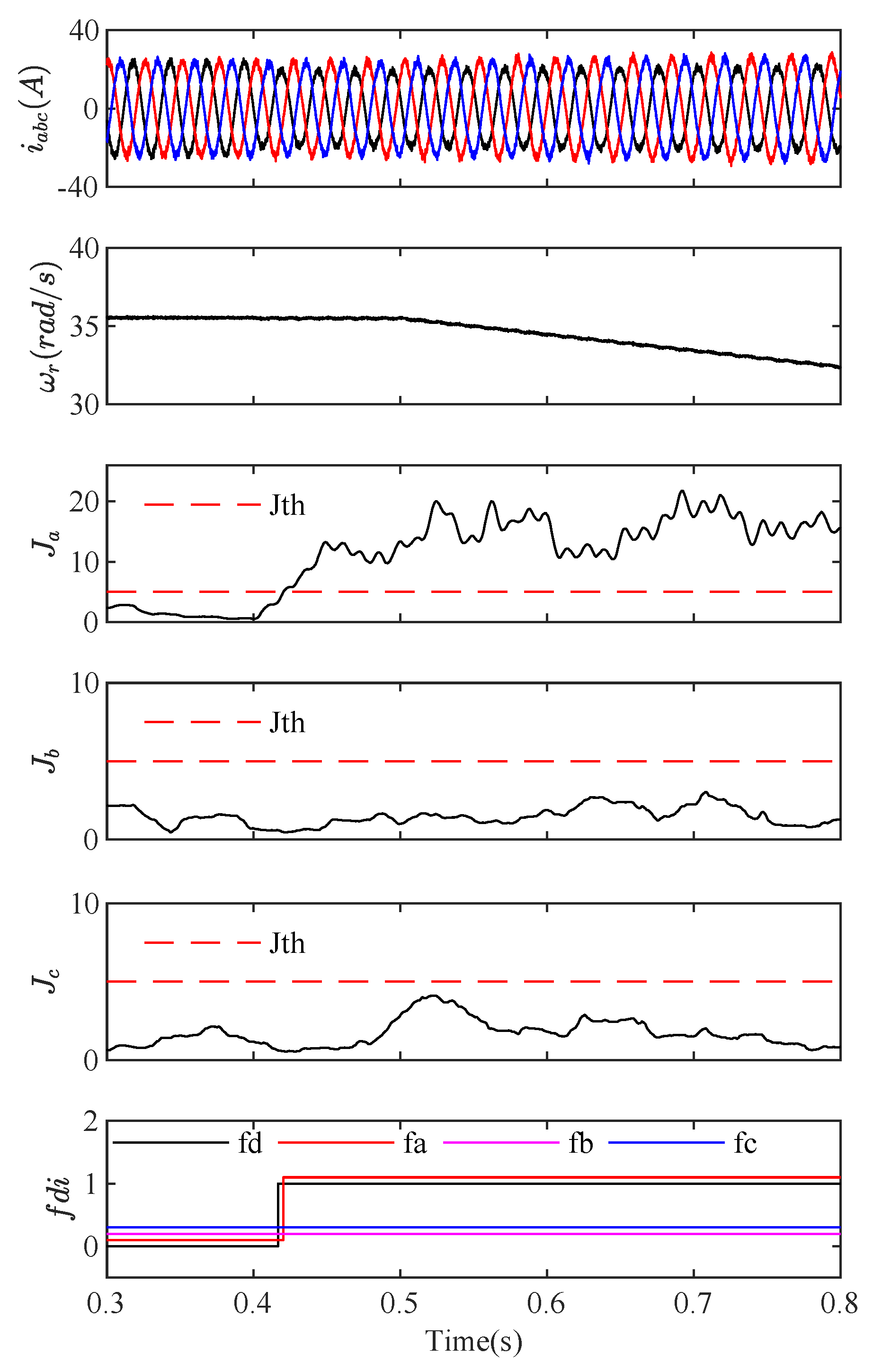
• Type a: gain error in phase a sensor, only 80% of the measured value fed to the controller,
• Type b: bias fault in phase b sensor, 4 A is added to the measured value,
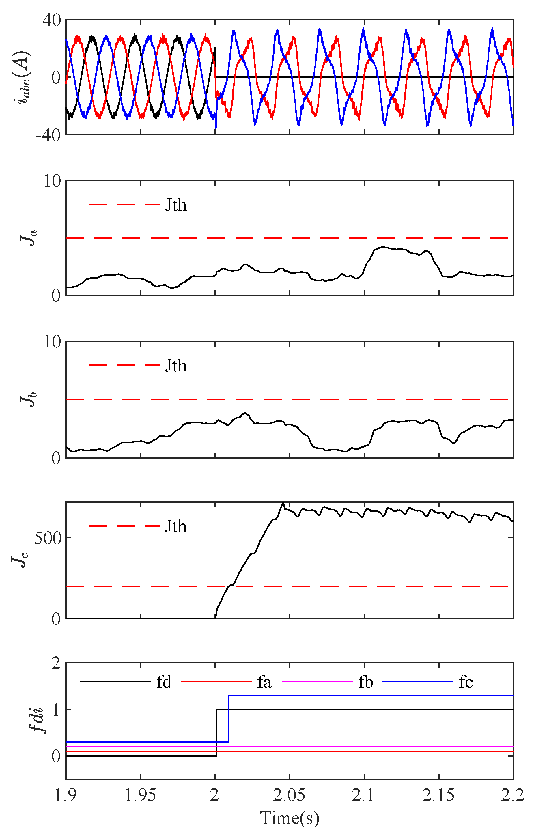
• Type c: disconnection of phase c sensor, the measurement output becomes zero.

Type a fault is modeled as multiplicative fault, Type b and Type c are additive faults. These faults are commonly presented in literature and practice applications.

The proposed method generates three fault isolation variables $J_a$, $J_b$,$J_c$ and a detection flag $f_d$. $f_a$, $f_b$ and $f_c$ denote the isolation flags related to $J_a$, $J_b$ and $J_c$. When the detection observer detects fault in the system, $f_d$ changes from ‘0’ to ‘1’. Only when the isolation variables $J_a$, $J_b$ and $J_c$ exceed the defined thresholds will the corresponding isolation flags change from ‘0’ to ‘1’.

5.1. Performance for Single Sensor FDI with External Disturbance

The mechanical power fed to generator varies slowly to simulate real wind power in all simulation. Type a and type c fault occur at $t=0.4$ s and $t=2.0$ s as shown in Figure 3 and Figure 4. Fault detection variable $f_d$ changes instantly and corresponding isolation flag $f_a$ and $f_c$ change subsequently at $t=0.42$ s and $t=2.01$ s. In addition, the mechanical power variation starts at $t=0.5$ s, which causes sudden variation of the rotor speed. During this period, $f_d$ and $f_a$ remain higher than the threshold while $f_b$ and $f_c$ are lower than detection threshold, which indicates that the isolation algorithm is robust to the disturbances.

The current waveforms of the healthy phase will be distorted by the faulty sensor because of feedback control. As shown in Figure 4, Type c fault of phase c current sensor distorts phase a and phase b currents. When phase c fault is triggered at $t=2$ s, fault detection flag $f_d$ and isolation flag $f_c$ change from ‘0’ to ‘1’ while $f_a$ and $f_b$ remain ‘0’. This reports that the proposed isolation variables are only sensitive to the corresponding fault phase and makes it possible to isolate all phase current sensor faults. The next section will show the multiple sensor fault diagnosis performance.

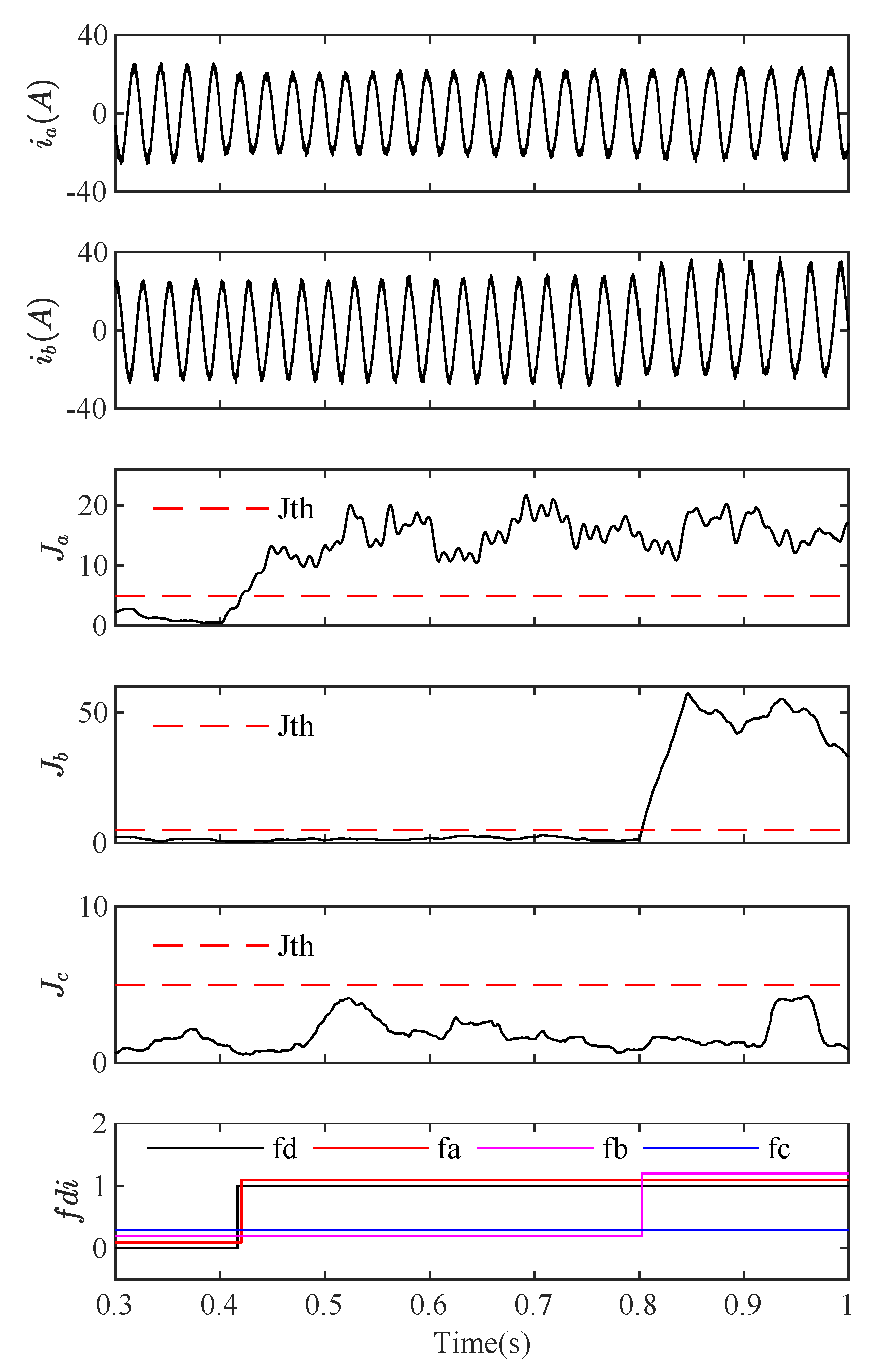
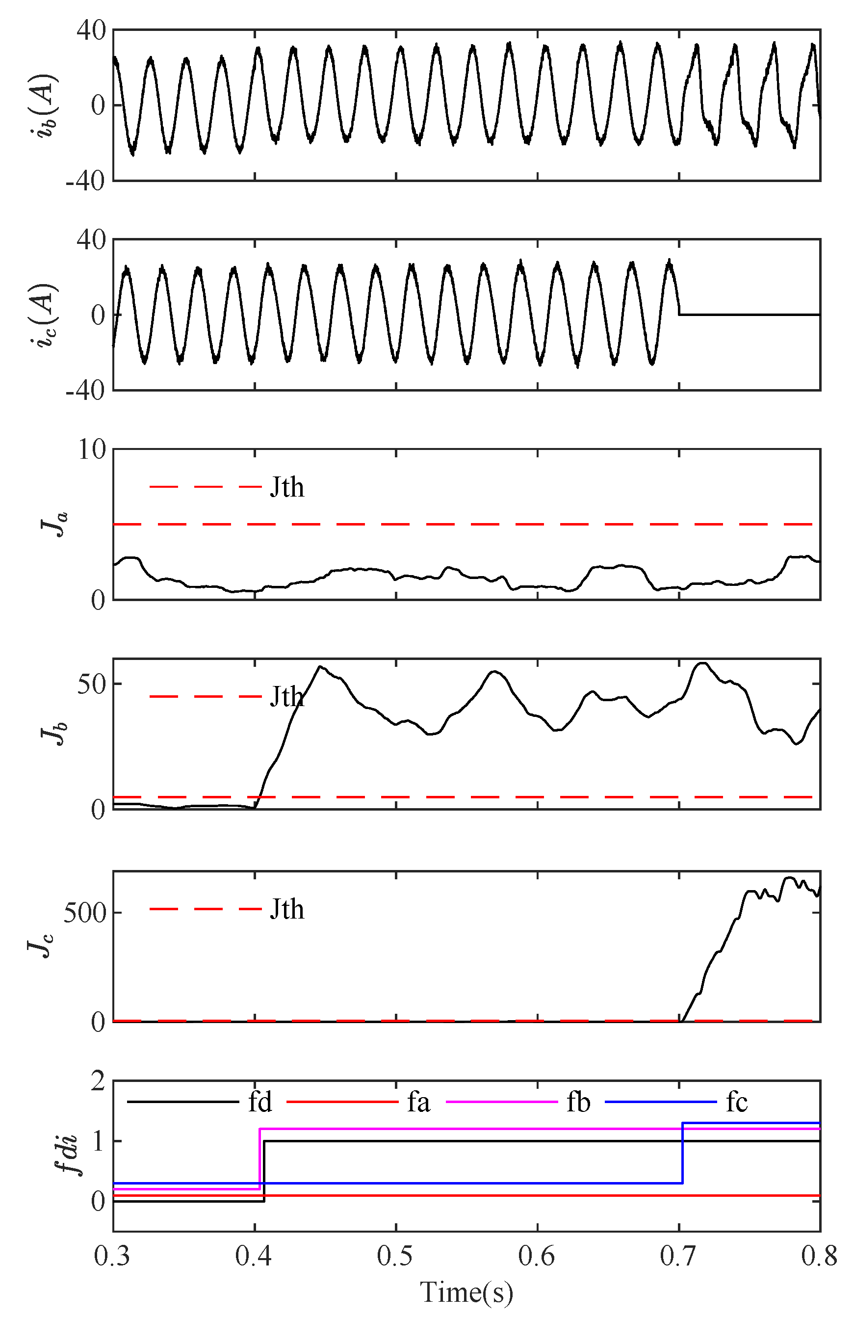
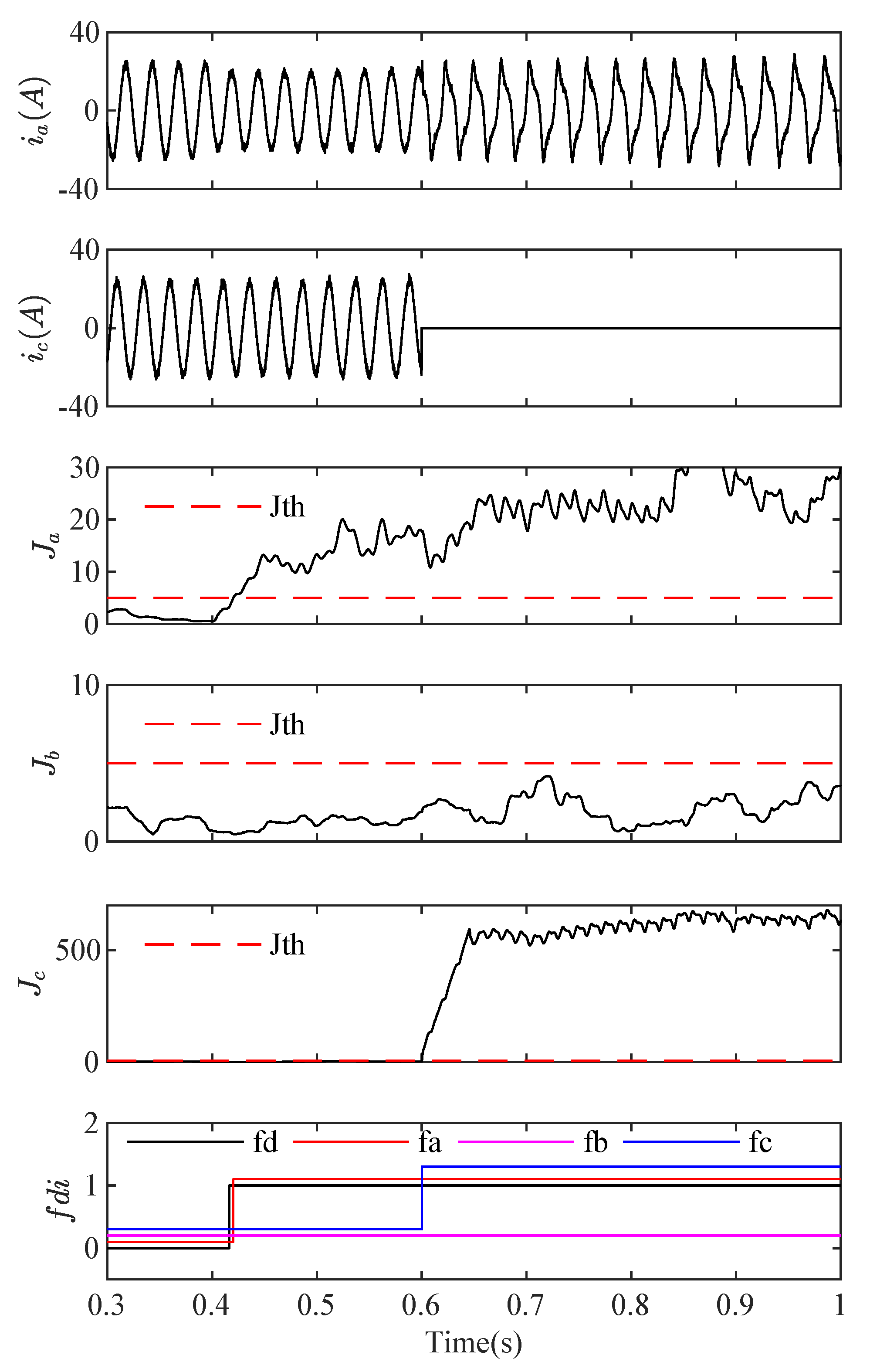
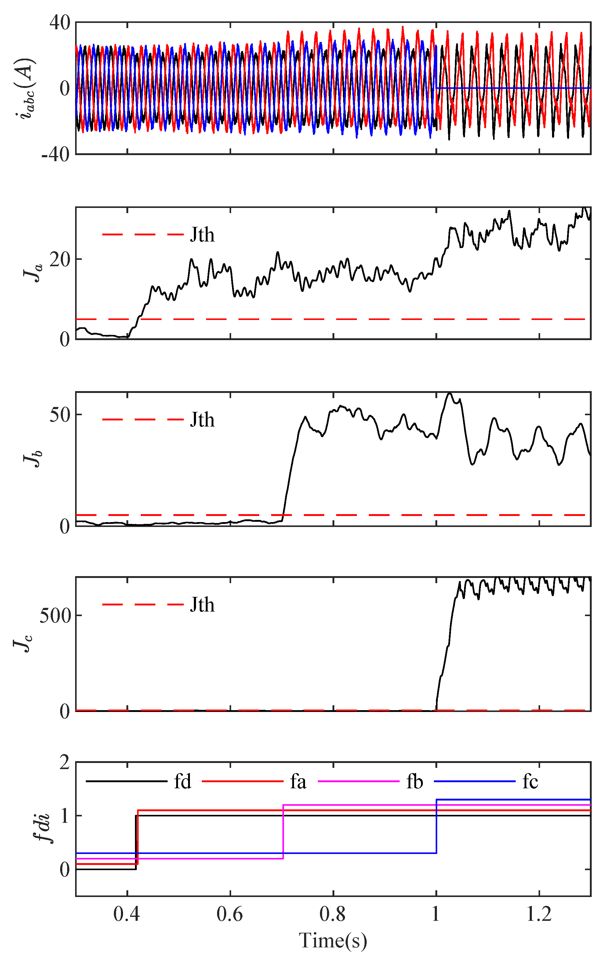
5.2. Multiple Fault Detection and Isolation

Multiple sensor FDI scenarios are presented as follows:

• Type a and Type b fault at $t=0.4$ s and $t=0.8$ s,
• Type b and Type c fault at $t=0.4$ s and $t=0.7$ s,
• Type a and Type c fault at $t=0.4$ s and $t=0.6$ s,
• Three type faults occur simultaneously at $t=0.4$ s, $t=0.7$ s and $t=1.2$ s.

The FDI variable behaviors during multiple current sensor faults are shown in Figure 5, Figure 6, Figure 7 and Figure 8. The fault detection flag $f_d$ and isolation flags $f_a$, $f_b$, $f_c$ change from ‘0’ to ‘1’ after the faults occurred. For two sensor fault scenarios, the isolation flag for healthy sensor remains ‘0’, indicating that it operates normally.

5.3. Comparison with the Existing Sensor FDIs

Table 2. Comparison of a model-based current sensor FDI scheme.

FD Scheme	Measurements	Fault Types	Isolability	System Model	Detection Variables
Bank of observers [28]	1 voltage, 3 currents, 1 speed	Type c	Single	IM model in $\alpha -\beta$	Estimation errors of rotor flux and speed
EKF [29]	1 voltage, 2 currents, 1 speed	Type c	Single	IM model in $\alpha -\beta$	Estimation errors of phase currents
Adaptive observer [30]	1 voltage, 2 currents, 1 speed	Type c	Single	IM model in $d-q$	Fault inference based on current errors
Bank of observers [8]	1 voltage, 2 currents, 1 speed	Type a, Type b, Type c	2 faults	IM model in $\alpha -\beta$	Geometric residuals
TS fuzzy observers [9]	2 currents, 1 speed	Type b	2 faults	DFIG model in $\alpha -\beta$	Estimation errors of the states
Integrated ${\mathcal{H}}_{\_}/{\mathcal{H}}_{\infty }$ filters [10]	2 currents, 1 speed, 1 position	Type a, Type b, Type c	2 faults	DFIG model in $d-q$ and $\alpha -\beta$	Generalized likelihood ratio of residuals
TVKF [2]	2 currents, 1 speed	Type a, Type b, Type c	3 faults	PMSG model in harmonic domain	Generalized likelihood ratio of residuals
Sliding mode observer [31]	3 currents, 1 speed, 1 position	Type c	2 faults	PMSG model in $d-q$	Evaluation of estimation errors
This method	3 currents, 1 speed, 1 position	Type a, Type b, Type c	3 faults	PMSG model in $\alpha -\beta$	Evaluation of the fault estimates

presents a brief comparison of model-based current sensor FDIs. These schemes are proposed for an IM system [8,28,29,30], DFIG system [9,10] and PMSG system [2,31]. The schemes in [28,29,30] are presented to isolate single sensor fault. In these approaches, a bank of observers is established to monitor each sensor fault on the basis of the rest sensors are health. T-S fuzzy observer [9] and sliding mode observer [31] are proposed to isolate single type of faults in $\alpha -\beta$ and $d-q$ frame. The measurements of three-phase currents are utilized to generate estimation errors that can only isolate faults in a stationary frame or synchronous reference frame. The TVKF scheme is presented for the PMSG system in [2]. It utilizes a generalized likelihood ratio maximum-shift strategy to evaluate the faulty residuals generated by the frequency domain model, which results in higher computation complexity. This work is presented for multiple sensor fault isolation of PMSG or PMSM based system with a simple observer based algorithm framework. In general, the proposed method can detect and isolate multiple sensor faults simultaneously in a short diagnosis time. It employs mechanical signals and current signals in the control loop without any additional measurements and hardware circuits, and can be integrated into the control loop. In addition, it shows excellent performance in multiple types of faults including gain fault, biased fault, and disconnection fault. The fault detection threshold is related to disturbances with respect to Theorem 1 and Theorem 2. Furthermore, the maximum and minimum power for WECSs are specifically defined by the operational region shown in Figure 2.

5.4. Discussions

In this paper, only simulation results are presented to validate the FDI performance. The proposed scheme is designed for online operation and is independent from control strategies. Some essential issues are discussed with respect to the lack of experimental results.

• The component parameters of simulation model come from the real laboratory prototype with rated power 2.5 kW. Its controller parameters are designed on the simulation file and can guarantee the control performance. The real waveforms and power characteristics are the same as those of simulation results. The observer design is a dual problem of controller design. Thus, the parameters designed in SIMULINK environment can be applied to the real experiments.
• The threshold selection is the most challenging problem in implementing the proposed algorithm. In real application, the mechanical torque and measurement noise are different from the simulation configuration. This will be further introduced into the observer and error dynamics. These effects can be modeled as generalized unknown disturbances. The upper bound of the disturbances in real application is slightly different from simulation scenarios. However, this does not affect the performance since the upper bounds of disturbances and faults hold for real applications.
• The harmonics is another issue for current sensor fault diagnosis. The influences of harmonics on system behavior need to be further discussed with respect to system parameter and dynamics variation. However, few results have been presented for dealing with this problem, even for the controller designs in [20,21,22]. Recalling the FDI schemes in Table 2, only the method in [2] utilizes the harmonic model of PMSG to diagnose additive and multiplicative faults in current sensors. The state space model and output equation are linear combinations of each order harmonic in frequency domain, which indicates that the residuals can be modeled as the combination of finite harmonics. The proposed FDI takes the time domain behaviors of residuals into consideration. The average value of each fault estimate is calculated with a sliding window. Current sensor faults are evaluated via the threshold function defined in Equation (32). From this perspective, the harmonics will not affect the residual evaluation in time domain analysis.

6. Conclusions

In this paper, a robust observer based sensor FDI scheme, targeting both additive and multiplicative faults, is presented for PMSG in WECSs. This method isolates multiple sensor faults via two procedures: robust residual generation based fault detection and fault estimation based isolation. The system is reformulated as a LPV model in the $\alpha -\beta$ frame by introducing electromechanical dynamics of PMSG. The polytopic decomposition technique is applied to obtain the parameter-dependent form of the system model by defining a convex polytope with four vertices. Furthermore, the gain-scheduled residual generator and fault estimator are designed by ${\mathcal{H}}_{\infty }$ synthesis in the form of LMIs. The proposed gain-scheduled FDI scheme is capable of online monitoring of three-phase currents and isolating multiple sensor faults under varying disturbances.

The proposed scheme is implemented in a MATLAB/SIMULINK environment and multiple sensor faults are isolated correctly. Due to the lack of experimental validation, the corresponding issues are discussed in Section 5.4, of which the challenging issue is the influence of disturbances and harmonics on threshold selection and system dynamics. In a real power conversion system, the diagnosis thresholds in (32) need to be investigated further by defining the augmented disturbances including measurement noise and parameter uncertainties. However, it does not affect the theoretical results of Theorem 1 and Theorem 2 since the observability of the pair $\left(A\left({\theta }_k\right),C\right)$ and $\left(\overline{A}\left({\theta }_k\right),\overline{C}\right)$ is independent of disturbances. Since further results is lacked about the influence of harmonics on system dynamics, it is difficult to quantify these effects on the system. The results in [20,21,22] indicate that the gain-scheduled controller design based on the this LPV model suffers less from the harmonics. Observer design as the dual problem of controller design is less dependent on the harmonic problem.

In addition, fault estimates are sensitive enough to distinguish each phase current sensor fault but cannot be applied directly for the purpose of fault compensation because of the unknown disturbances. The future work will be focused on the unbiased fault estimation and fault tolerant control for PMSG based WECS system on the basis of this LPV modeling technology.

References

1. Wu, C.; Guo, C.; Xie, Z.; Ni, F.; Liu, H. A Signal-Based Fault Detection and Tolerance Control Method of Current Sensor for PMSM Drive. IEEE Trans. Ind. Electron. 2018, 65, 9646–9657. [Google Scholar] [CrossRef]
2. Beddek, K.; Merabet, A.; Kesraoui, M.; Tanvir, A.A.; Beguenane, R. Signal-Based Sensor Fault Detection and Isolation for PMSG in Wind Energy Conversion Systems. IEEE Trans. Instrum. Meas. 2017, 66, 2403–2412. [Google Scholar] [CrossRef]
3. Song, Y.; Wang, B. Survey on Reliability of Power Electronic Systems. IEEE Trans. Power Electron. 2013, 28, 591–604. [Google Scholar] [CrossRef]
4. Yang, Z.; Chai, Y. A survey of fault diagnosis for onshore grid-connected converter in wind energy conversion systems. Renew. Sustain. Energy Rev. 2016, 66, 345–359. [Google Scholar] [CrossRef]
5. Yang, S.; Xiang, D.; Bryant, A.; Mawby, P.; Ran, L.; Tavner, P. Condition Monitoring for Device Reliability in Power Electronic Converters: A Review. IEEE Trans. Power Electron. 2010, 25, 2734–2752. [Google Scholar] [CrossRef]
6. Rothenhagen, K.; Fuchs, F.W. Current Sensor Fault Detection, Isolation, and Reconfiguration for Doubly Fed Induction Generators. IEEE Trans. Ind. Electron. 2009, 56, 4239–4245. [Google Scholar] [CrossRef]
7. Rothenhagen, K.; Fuchs, F.W. Doubly Fed Induction Generator Model-Based Sensor Fault Detection and Control Loop Reconfiguration. IEEE Trans. Ind. Electron. 2009, 56, 4229–4238. [Google Scholar] [CrossRef]
8. Aguilera, F.; de la Barrera, P.; Angelo, C.D.; Trejo, D.E. Current-sensor fault detection and isolation for induction-motor drives using a geometric approach. Control Eng. Pract. 2016, 53, 35–46. [Google Scholar] [CrossRef]
9. Abdelmalek, S.; Barazane, L.; Larabi, A.; Bettayeb, M. A novel scheme for current sensor faults diagnosis in the stator of a DFIG described by a T-S fuzzy model. Measurement 2016, 91, 680–691. [Google Scholar] [CrossRef]
10. Boulkroune, B.; Gálvez-Carrillo, M.; Kinnaert, M. Combined Signal and Model-Based Sensor Fault Diagnosis for a Doubly Fed Induction Generator. IEEE Trans. Control Syst. Technol. 2013, 21, 1771–1783. [Google Scholar] [CrossRef]
11. Akrad, A.; Hilairet, M.; Diallo, D. Design of a Fault-Tolerant Controller Based on Observers for a PMSM Drive. IEEE Trans. Ind. Electron. 2011, 58, 1416–1427. [Google Scholar] [CrossRef]
12. Mwasilu, F.; Jung, J. Enhanced Fault-Tolerant Control of Interior PMSMs Based on an Adaptive EKF for EV Traction Applications. IEEE Trans. Power Electron. 2016, 31, 5746–5758. [Google Scholar] [CrossRef]
13. Kommuri, S.K.; Defoort, M.; Karimi, H.R.; Veluvolu, K.C. A Robust Observer-Based Sensor Fault-Tolerant Control for PMSM in Electric Vehicles. IEEE Trans. Ind. Electron. 2016, 63, 7671–7681. [Google Scholar] [CrossRef]
14. Kommuri, S.K.; Lee, S.B.; Veluvolu, K.C. Robust Sensors-Fault-Tolerance With Sliding Mode Estimation and Control for PMSM Drives. IEEE/ASME Trans. Mech. 2018, 23, 17–28. [Google Scholar] [CrossRef]
15. Foo, G.H.B.; Zhang, X.; Vilathgamuwa, D.M. A Sensor Fault Detection and Isolation Method in Interior Permanent-Magnet Synchronous Motor Drives Based on an Extended Kalman Filter. IEEE Trans. Ind. Electron. 2013, 60, 3485–3495. [Google Scholar] [CrossRef]
16. Wang, Y.; Meng, J.; Zhang, X.; Xu, L. Control of PMSG-Based Wind Turbines for System Inertial Response and Power Oscillation Damping. IEEE Trans. Sustain. Energy 2015, 6, 565–574. [Google Scholar] [CrossRef] [Green Version]
17. Badihi, H.; Zhang, Y.; Hong, H. Wind Turbine Fault Diagnosis and Fault-Tolerant Torque Load Control Against Actuator Faults. IEEE Trans. Control Syst. Technol. 2015, 23, 1351–1372. [Google Scholar] [CrossRef]
18. Bifaretti, S.; Iacovone, V.; Rocchi, A.; Tomei, P.; Verrelli, C. Nonlinear speed tracking control for sensorless PMSMs with unknown load torque: From theory to practice. Control Eng. Pract. 2012, 20, 714–724. [Google Scholar] [CrossRef]
19. Tomei, P.; Verrelli, C.M. Observer-Based Speed Tracking Control for Sensorless Permanent Magnet Synchronous Motors With Unknown Load Torque. IEEE Trans. Autom. Control 2011, 56, 1484–1488. [Google Scholar] [CrossRef]
20. Kang, C.M.; Lee, S.; Chung, C.C. Discrete-Time LPV 2 Observer With Nonlinear Bounded Varying Parameter and Its Application to the Vehicle State Observer. IEEE Trans. Ind. Electron. 2018, 65, 8768–8777. [Google Scholar] [CrossRef]
21. Lee, Y.; Lee, S.; Chung, C.C. LPV Control with Disturbance Estimation for Permanent Magnet Synchronous Motors. IEEE Trans. Ind. Electron. 2018, 65, 488–497. [Google Scholar] [CrossRef]
22. Lee, Y.; Shin, D.; Kim, W.; Chung, C.C. Nonlinear 2 Control for a Nonlinear System With Bounded Varying Parameters: Application to PM Stepper Motors. IEEE/ASME Trans. Mech. 2017, 22, 1349–1359. [Google Scholar] [CrossRef]
23. De Souza, C.E.; Barbosa, K.A.; Neto, A.T. Robust filtering for discrete-time linear systems with uncertain time-varying parameters. IEEE Trans. Signal Process. 2006, 54, 2110–2118. [Google Scholar] [CrossRef]
24. Pandey, A.P.; de Oliveira, M.C. Discrete-time control of linear parameter-varying systems. Int. J. Control 2018. [Google Scholar] [CrossRef]
25. Pandey, A.P.; de Oliveira, M.C. A new discrete-time stabilizability condition for Linear Parameter-Varying systems. Automatica 2017, 79, 214–217. [Google Scholar] [CrossRef]
26. Pandey, A.P.; de Oliveira, M.C. On the Necessity of LMI-Based Design Conditions for Discrete Time LPV Filters. IEEE Trans. Autom. Control 2018, 63, 3187–3188. [Google Scholar] [CrossRef]
27. Li, L.; Ding, S.X.; Qiu, J.; Yang, Y.; Zhang, Y. Weighted Fuzzy Observer-Based Fault Detection Approach for Discrete-Time Nonlinear Systems via Piecewise-Fuzzy Lyapunov Functions. IEEE Trans. Fuzzy Syst. 2016, 24, 1320–1333. [Google Scholar] [CrossRef]
28. Yu, Y.; Wang, Z.; Xu, D.; Zhou, T.; Xu, R. Speed and Current Sensor Fault Detection and Isolation Based on Adaptive Observers for IM Drives. J. Power Electron. 2014, 14, 967–979. [Google Scholar] [CrossRef] [Green Version]
29. Zhang, X.; Foo, G.; Vilathgamuwa, M.D.; Tseng, K.J.; Bhangu, B.S.; Gajanayake, C. Sensor fault detection, isolation and system reconfiguration based on extended Kalman filter for induction motor drives. IET Electr. Power Appl. 2013, 7, 607–617. [Google Scholar] [CrossRef]
30. Najafabadi, T.A.; Salmasi, F.R.; Jabehdar-Maralani, P. Detection and Isolation of Speed-, DC-Link Voltage-, and Current-Sensor Faults Based on an Adaptive Observer in Induction-Motor Drives. IEEE Trans. Ind. Electron. 2011, 58, 1662–1672. [Google Scholar] [CrossRef]
31. Saha, S.; Haque, M.E.; Mahmud, M.A. Diagnosis and Mitigation of Sensor Malfunctioning in a Permanent Magnet Synchronous Generator Based Wind Energy Conversion System. IEEE Trans. Energy Convers. 2018, 33, 938–948. [Google Scholar] [CrossRef]
Figure 1. Control and fault diagnosis scheme for the PMSG system (reproduced from [2,16]).
Applsci 08 01816 g001
Figure 2. Operation regions of a PMSG based wind turbine (reproduced from [17]).
Applsci 08 01816 g002
Figure 3. Simulation results on the single phase fault isolation, under varying mechanical disturbance (from top to bottom are phase a current i a b c , rotor speed ω r , isolation variables f a , f b , f c and FDI flags).
Applsci 08 01816 g003
Figure 4. Simulation results for fault isolation of Type c fault in phase c (from top to bottom are three-phase current i a b c , isolation variables f a , f b , f c and FDI flags f d , f a , f b , f c ).
Applsci 08 01816 g004
Figure 5. Simulation results on simultaneous isolation of phase a and phase b fault.
Applsci 08 01816 g005
Figure 6. Simulation results on simultaneous isolation of phase b and phase c fault.
Applsci 08 01816 g006
Figure 7. Simulation results on simultaneous isolation of phase a and phase c fault.
Applsci 08 01816 g007
Figure 8. Simulation results on simultaneous isolation of three-phase sensor faults.
Applsci 08 01816 g008